Improved Prediction of Periodicity Using Quartet Approximation in a Lattice Model of Intracellular Calcium Release

1. Introduction

Probabilistic cellular automata (PCA), a class of binary lattice models, are fairly ubiquitous in modeling complex systems (along with agent-based models), in fields ranging from physics to ecology to economics [for a selection of examples see [1]]. While their appeal stems from their intuitive, bottom-up approach in which the local interactions of randomly-acting particles, agents, or other units are explicitly represented, their importance is in revealing large-scale (macroscopic) phenomena that result in unexpected ways from the various local (microscopic) actions.

Successfully explaining and predicting these macroscopic behaviors with less computationally-intensive and more analytic methods is the subject of much active research. Using one such class of methods, moment closure [2], one may create a closed-form expression that models the time-evolving probability for the future states of the PCA lattice. In the most common version of this approach, the zero-order mean-field approximation (MFA), the probabilistic state of a single, randomly-selected site in the lattice is modeled using a single difference equation. Although this method is commonly used and often straightforward to apply, it ignores all spatial correlation information by treating all neighbors as “average,” and may provide incorrect results when spatial interactions are fundamental to the long-term dynamics. In higher-order versions, the joint state of larger structures is explicitly modeled using coupled difference equations, while still treating yet more distant neighbors as average. These larger structures can be a pair of sites (first-order nearest-neighbor correlations), or a triplet or quartet of sites (second-order neighbor-of-neighbor correlations), or even larger. Their use may be necessary to fully capture certain dynamics of the underlying model, but at the cost of increased mathematical complexity and higher computational load, due to the fact that the set of possible configurations (and thus the number of difference equations) grows exponentially with the size of the structure being considered. Correctly calculating the probabilities for each configuration requires a careful and systematic approach. Pair approximation approaches for spatial lattice models were originally introduced in the physics community [3, 4] and have since been used in a wide array of fields such as ecology [5], epidemiology [6], and political theory [7]. Higher-order approximations have also been successfully used in models for, e.g., ecological dispersion [8, 9] and viral spread in epidemiology [10].

The PCA model analyzed in the present study was originally developed [11–13] to study the dynamics of intracellular calcium release in cardiac myocytes, the cells that make up the muscle tissue of the heart. Within each of these cells, calcium ions are discharged from internal storage into the main cellular compartment via a lattice-like arrangement of calcium release units (CRUs) [14]. Numbering in the tens of thousands in a typical myocyte, each CRU behaves as an excitable element, where a small triggering signal provided by the voltage-mediated excitation at the beginning of the heartbeat can result in a local release of that CRU's calcium load (self-activation). However, this activation is stochastic only, due to the thermodynamic noise of the associated ion channels, therefore only a portion of CRUs may respond with self-activation. Additionally, as calcium itself serves as another triggering mechanism, the released ions from self-activated CRUs can diffuse to neighboring CRUs and induce them to undergo release, in a process called recruitment (also a stochastic process). The end result is that a certain percentage of CRUs in the cell have been activated at the completion of each heartbeat. Of particular interest is the clinically-and physiologically-important phenomenon of calcium alternans [15], a dynamic feature of the cell in which there is a beat-to-beat alternation between high and low percentage of CRU activation [see [16] for a brief review of experimental evidence]. Because calcium plays a central role in cardiac excitation-contraction coupling, alternans is an important factor in various known electrocardiac markers associated with an increased risk of sudden cardiac death [17].

In Rovetti et al. [11] and Cui et al. [12] we used the PCA model to suggest a mechanism for the production of alternans wherein excitable elements were subject to both randomness and spatial interaction (recruitment) consistent with the known behavior of cardiac myocytes. Our PCA model was able to qualitatively reproduce the phenomenon of periodic alternans. We then applied an MFA analysis to show that, under appropriate conditions, the PCA dynamics experience a bifurcation to period-2 behavior, mimicking the high-low pattern seen in physiological alternans. However, by its nature, the mean-field approximation ignores spatial correlations, and in that analysis there were quantitative differences between the MFA and the PCA for the predicted onset of periodic alternans. Furthermore, by ignoring spatial coupling, the mean-field approximation cannot predict the emergence of spatial correlations, which is also observed in the lattice model. Significant spatial patterning, in the form of spatially-discordant calcium alternans, has been observed experimentally [18, 19] in cardiac myocytes; thus, providing a theoretical basis for further analysis is also of interest.

In this study we apply the method of pair and quartet approximations to extend the original MFA analysis of the PCA model. We show that the second-order quartet approximation is able to more accurately predict the onset of periodic behavior (alternans), and also predicts the emergence of spatial clustering (absent in the original MFA analysis). The successful implementation of the quartet approximation provides a framework for possible further research into the dynamics of pattern formation in the spatio-temporal dynamics of probabilistic cellular automata.

2. Lattice Model

2.1. Model Description

We begin with an N × N square lattice (Figure 1A) in which each site can be in one of two states (0, “inactive,” or 1, “active”). Each site has four nearest neighbors, except for edge sites (three neighbors) and corner sites (two neighbors). Time proceeds in discrete steps, and during each step the states of all sites are updated synchronously according to a set of probabilistic transition rules. Inactive sites may remain inactive, or they may transition to active either by self-activation or by recruitment; the latter relies on interaction with nearest neighbors, while the former does not. Active sites are required to transition to inactive on the next beat, thereby preventing sites from activating twice in two consecutive beats; this refractoriness property is also consistent with CRU physiology.

FIGURE 1

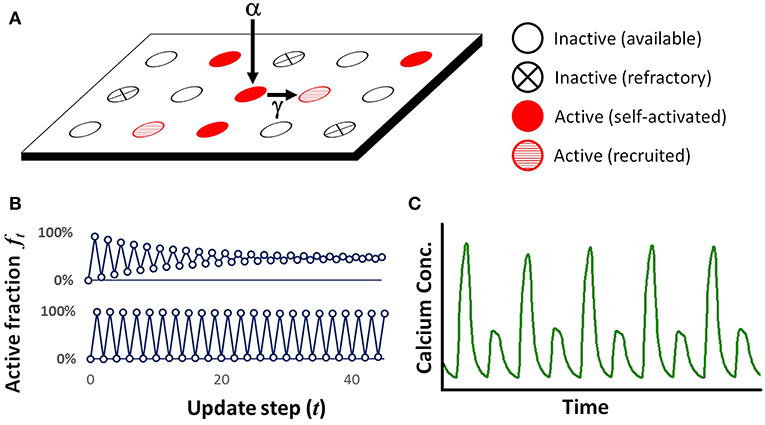
Figure 1. (A) Illustration of lattice arrangement and possible states in the PCA. Available sites can self-activate with probability α, or be recruited with probability γ. (B) Example of PCA lattice simulation showing the activation fraction f_t reaching either a steady state (top, for γ = 0.25) or maintaining periodicity (bottom, for γ = 0.75). In both cases α was fixed at 0.80. (C) Simplified graphical representation of a typical experimental recording of calcium concentration over time in a cardiac myocyte, under conditions that produce alternans. Each peak represents either a high or low release of calcium, and peaks are ~ 150–300 ms apart.

A unique feature of these update rules is that recruitment by nearest neighbors can only occur after, and separate from, self-activation. Thus each update step is partitioned into two distinct substeps (see Figure 2):

FIGURE 2

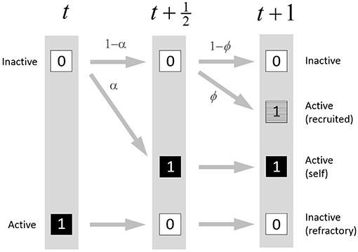
Figure 2. State transition diagram for the PCA model. In the first substep, inactive sites can self-activate with probability α. In the second substep, sites that are still inactive can be recruited to activate by their nearest neighbors with probability ϕ which depends on the number of nearest neighbors that activated during the first substep. Sites that begin the update step as active are forced to become inactive.

Substep 1. In this first substep (time t to $t+\frac{1}{2}$), each site that is available (non-refractory) is subject to self-activation, with probability α, a process that occurs independently of its neighboring sites. On the other hand, any site that enters the update step as active now becomes refractory, and therefore inactive. Refractory sites will again be eligible for activation on the next update step. All sites are updated synchronously during this substep.

Substep 2. In the second substep (time $t+\frac{1}{2}$ to t + 1), a site that is available (non-refractory) and is still inactive may be recruited by neighbors that self-activate during substep 1. Each active neighbor independently attempts to recruit the site with probability γ. (The site need be recruited only once, and once it is recruited it is considered to be active.) The total probability ϕ that the site will be recruited to the active state by any available neighbor is given by ϕ = 1 − (1 − γ)^s where s ∈ {0, …, 4} is the number of nearest neighbors that are active after substep 1. Sites are updated synchronously during this substep also; recruited sites cannot go on to recruit additional sites within the same update step.

At the end of the update step, sites are considered to be either active (whether by self-activation, or by recruitment) or inactive (whether by failure to activate, or by being refractory following an activation in the preceding update step). All sites that activate in the current update step will be refractory (inactive) in the next update step.

2.2. Measures of Interest

There are two primary phenomena of interest concerning the ensemble behavior of the lattice as a whole. The first is periodicity in the ensemble activation as measured by the fraction f_t of sites in the active state. The macroscopic quantity f_t can undergo a transition from steady-state to period-2 behavior (see Figure 1B) under appropriate conditions such as a suitably strong spatial coupling force as supplied by the recruitment probability γ. The activation fraction f_t is meant to represent qualitatively the peak amount of calcium that is released during a single heartbeat in an experimentally-observed myocyte (Figure 1C). Our measure of the extent of the periodicity will be the amplitude of the beat-to-beat change, A_t = |f_t − f_{t − 1}| (Note that in all simulation and computations, steady-state and periodic should be understood as meaning quasi-steady-state and quasi-periodic, respectively, as the presence of stochastic noise means that the value of A_t will exhibit a small degree of variability from beat to beat even under “steady-state” conditions).

The second phenomenon is spatial clustering, or spatial correlation, the tendency for sites to be found next to sites of like state, resulting in the emergence of pattern formation over time. We employ a clustering coefficient Q to measure this phenomenon. Let $f_t^{con}$ be the fraction of total nearest-neighbor pairs in the lattice which are concordant (in like states, either both inactive or both active). Then we define

$Q_t=\frac{f_t^{con}}{f_t^2+{(1-f_t)}^2}-1.$

The ratio term compares the observed concordance fraction to the expected concordance fraction under the assumption of independent random assortment of active sites. Q_t can range from Q_t = −1 (complete anti-clustering, i.e., a repulsive force) to Q_t = 0 (random assortment with no spatial clustering) to Q_t = 1 (complete clustering). However, regardless of the value of $f_t^{con}$, the value of Q_t will become 0 as f_t approaches 0 or 1, reflecting the fact that as the lattice approaches a state of being all inactive or all active, the concept of clustering no longer applies in a meaningful way.

2.3. Simulation Methods

A lattice size of N = 200 was used for all numerical simulations of the PCA. All computations for both the PCA and the subsequent approximation methods were carried out for at least 500,000 update steps in order to ensure achieving a stationary state. While the alternation in f_t usually became apparent within the first 100 update steps, this allowed sufficient time for spatial clustering patterns to develop. The initial condition at t = 0 was to have all sites in the lattice set to inactive. All computations were performed on a 256-core Beowulf cluster using GNU C++ v4.8.5 with the Armadillo linear algebra library v8.3 [20] and the XOR128 pseudo-random number generator [21], which has a period of 2³² − 1.

2.4. Simulation Results

Our previous studies [11] have demonstrated that periodic behavior occurs only for sufficiently high values of both α and γ. For simplicity of presentation in this section, we fix the self-activation probability α to a high value (α = 0.80) and explore a range of values for the recruitment probability γ. Figure 1B shows the initial time-course of f_t in the cases where the lattice reaches a steady-state (for γ = 0.25) or periodicity (for γ = 0.75). While the behaviors are fairly quickly established, a small level of random noise persists. Full lattices are shown in Figure 3 at two consecutive update steps for a range of values of the recruitment probability γ. At γ = 0.25, a typical value for which little spatial clustering or alternation is present, we see that about half of the sites are active. As γ is increased to 0.65, some clustering becomes apparent but alternation is still absent. By γ = 0.74 the spatial clustering is very noticeable. From γ = 0.74 to γ = 0.76 there is a sudden and sharp increase in the alternation of f_t, and the expected decrease in spatial clustering as f_t reaches extreme values. There appears to be a transition point in the behavior of the system at around γ ≈ 0.75 (however this transition point is also dependent on α as is shown later in section 6).

FIGURE 3

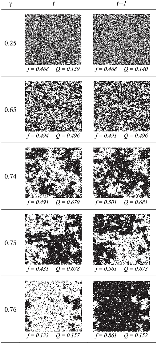
Figure 3. Simulation results in the PCA after 500,000 update steps, for five different values of γ (recruitment probability). Black is active and white is inactive. The left and right panels in each row are two consecutive time steps. The active fraction f begins to alternate around γ = 0.75. Spatial clustering (Q) increases as γ increases, and is strongest immediately before the onset of alternation (periodicity). In all cases, α was fixed at 0.80.

3. Mean-Field Approximation

The goal of the mean-field approximation (MFA) is to predict the activation fraction f_t with the single-site activation probability p_t by ignoring all spatial correlation information and assuming that all sites are decoupled. In this sense, all sites are equivalent and behave in a unified manner as a single “average” site, with a probability p_t of being found in the active state.

The MFA has previously been derived for this PCA model [11, 12] and we summarize it here. Let p_t be the probability that a single site will be found in the active state at time t. Then the MFA yields the difference equation

$\begin{array}{ll}{p}_{t+1}=\left(1-p_t\right)\left[\alpha +\left(1-\alpha \right){\xi }_t\right]& (1)\end{array}$

where (1 − p_t) is the probability the site will be available (non-refractory) for activation, (1 − α) is the probability that it does not self-activate, and ${\xi }_t=1-{\left[1-\alpha \gamma (1-p_t)\right]}^4$ is the probability that the site will be recruited by any of four nearest neighbors.

Implicit in ξ_t is the fundamental assumption of the mean-field approximation, which is that the nearest neighbors are treated as being randomly sampled from the lattice; as such, neighbors are available to recruit at the average rate 1 − p_t, will activate at the average rate α, and finally will successfully recruit at the average rate γ. The amplitude of the beat-to-beat change in the activation probability is given by A_t = |p_t − p_{t − 1}| for the MFA model.

4. Pair Approximation

Pair approximation replaces the single-site probability p_t with a family of two-site probabilities P_t[ab], where a and b represent a spatially-adjacent pair of sites, each of which can be either active or inactive (i.e., a, b ∈ {0, 1}). This leads to four difference equations corresponding to the terms P_t [00], P_t [01], P_t [10], and P_t [11] satisfying $\sum _{a,b}{P}_t\left[ab\right]=1$. While the number of equations has increased, the payoff is that some information about the state of a site's nearest neighbor is now explicitly incorporated.

Refer to Figure 4 for a visual representation of a pair of sites ab and the associated nearest neighbors. A pair in a spatially horizontal orientation is represented as [ab], while a pair in a vertical orientation is represented as $\left[\begin{array}{c}a\\ b\end{array}\right]$. We will use χ to represent the joint states of the entire local neighborhood of both the pair and their nearest neighbors. With two sites in a pair and six nearest neighbors, there are 2⁸ = 256 possible configurations for χ.

FIGURE 4

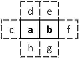
Figure 4. Template for the neighborhood χ consisting of the pair ab and its six nearest neighbors c through h. Each letter can take on the value 0 or 1.

In the calculations to follow we will make use of the marginal sums $P[a]={\displaystyle {\sum }_{b}P[ab].}$ We will also assume that the probabilities are symmetric with respect to spatial orientation, so that $P\left[ab\right]=p\left[\begin{array}{c}a\\ b\end{array}\right]=P\left[ba\right]=P\left[\begin{array}{c}b\\ a\end{array}\right]$.

4.1. Difference Equation

Let P_t [ab] and P_t [χ] be the probability of finding, respectively, the pair and the local neighborhood in the given state at time t (If the time dependence does not need to be explicitly shown, we write P_t as P for simplicity).

For any pair of sites, the probability that a particular configuration ab is achieved on the next update step t + 1 depends not only on the state of the pair at time t but the state χ of the entire local neighborhood. Let P [ab∣χ] be the production function, the probability that the local neighborhood χ can produce the pair ab during the next update step. Then, by conditioning on the neighborhood configuration χ, we can write the family of difference equations

$\begin{array}{ll}{P}_{t+1}[ab]={\displaystyle \sum _{\chi }P}[ab\mid \chi ]P_t[\chi ].& (2)\end{array}$

Equation (2) defines a set of four coupled difference equations, one for each pair configuration ab. Note that the production function P [ab∣χ] is time-independent, and the value of the term is determined solely by the update rules of the original lattice model; determining this function is a non-trivial process which we describe in section 4.3. The function P_t[χ], the neighborhood function, is the joint probability of the larger neighborhood, and we will be required to approximate it via closure methods, which we explore next.

4.2. Computing the Neighborhood Function

The local neighborhood χ for a pair contains sites that are third-order neighbors (i.e., three sites away). As discussed in the introduction, a closure approximation is required to estimate the joint probability of the eight sites in χ in terms of the first-order pair probabilities only.

To illustrate the general approach for closure as used by Filipe and Gibson [22] and Hiebeler [8], first consider as an example the second-order linear triplet of sites abc. If we ignore correlations between a and c and make the approximation that site c depends on site b but not on site a, then we can write

$P[abc]=P[ab]P[c\mid ab]\approx P[ab]P[c\mid b]=\frac{P[ab]P[bc]}{P[b]}.$

This establishes an approach whereby the joint probability of the larger structure abc can be approximated by covering (or “tiling”) the neighborhood with pairs ab and bc, and then dividing by the common site, or “overlap”, in this case b. The approach can be extended to arbitrarily large neighborhoods; for example, one third-order closure would be

$P[abcd]\approx \frac{P[ab]P[bc]P[cd]}{P[b]P[c]}$

The key observation is that higher-order correlations between more distant sites can be approximated in terms of the first-order (pairwise) terms.

Now considering a general neighborhood configuration χ, the probability P[χ] must be approximated using a closure method based upon first-order pair probabilities. There are many ways to tile the larger two-dimensional neighborhood structure via overlapping pairs; although each choice may produce slightly different approximations, no appreciable differences were noted when different choices were tested in this study. Hiebeler [8] lists all possible tilings which can be constructed using pairs; here we choose to use

$\begin{array}{ll}P[\chi ]=P\left[\begin{array}{c}de\\ cabf\\ hg\end{array}\right]\approx \frac{P[ca]P[da]P[de]P[eb]P[bf]P[bg]P[ah]}{P[a]P[d]P[e]P[b]P[b]P[a]}.& (3)\end{array}$

We refer to Equation (3) as the neighborhood function. The pair probabilities in the numerator of Equation (3) are known directly, and the single-site probabilities in the denominator can be computed as marginal sums.

4.3. Computing the Production Function

As mentioned in section 4.1, the production function P [ab | χ] must be carefully computed to adhere to the specific update rules of the lattice model. To achieve this in a systematic manner, we first summarize (Figure 5) the ways in which each possible ab configuration can be generated by an appropriate combination of self-activation and recruitment mechanisms. Because we are assuming rotational symmetry, it suffices to consider the equivalence classes of ab configurations under rotation, of which there are three; the representative configurations are [00], [10], and [11]. Then, for each class, we enumerate the ways in which that class could be generated via the mechanisms of activation as defined in the transition rules for the PCA. Each possible production pathway forms a subtype of that class. Finally, we indicate with symmetry multipliers the number of rotations that can appear within each class or within each subtype.

FIGURE 5

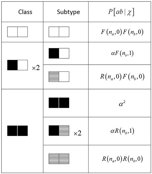
Figure 5. Table of complete configuration space for pair approximation. Each equivalence class is divided into one or more subtypes which are a combination of self-activation (black), recruitment (hatched), or inactive (white). n_a and n_b are the number of available non-pair neighbors to sites a and b, respectively. The symmetry multipliers (×2) account for rotation symmetry and indicate the number of cases to be considered.

For each subtype, we calculate the probability of its production, given the known nearest-neighbor states in its neighborhood χ, by multiplying the separate probabilities for each site in the pair. Recall that during any update step, a single inactive (non-refractory) site has one of three fates: self-activation, activation via recruitment, and failure to activate.

Self-activation. The probability that a site will activate on its own, which occurs independently of any neighboring sites, is given by α. Since this occurs during the first substep, no consideration of the second substep is necessary.

Recruitment. Within the context of a pair, the probability that a single site will be activated via the recruitment mechanism can be written

$R(n,j)=\left(1-\alpha \right)\left[1-{\left(1-\alpha \gamma \right)}^n{\left(1-\gamma \right)}^j\right].$

The initial term (1 − α) indicates failure to self-activate during the first substep. In order to compute whether the site will be recruited in the second substep, we need to have information about its four neighbors. One of its four neighbors is also the other member of the pair (i.e., a pair-neighbor), and we know its state explicitly. Let that state be j ∈ {0, 1}. Then the term (1 − γ)^j is the probability that this pair-neighbor will recruit the site. The states of the other three non-pair-neighbors obey the following: (1) with a specific neighborhood χ, we explicitly know how many of them will be available to activate, but (2) we can know whether they will successfully activate and recruit only probabilistically. Let n ∈ {0, 1, 2, 3} be the number of non-pair-neighbors which are available (i.e., non-refractory). Then the probability that any one of them will recruit the site is given by (1 − αγ)ⁿ.

Failure to activate. Using a similar line of reasoning, the probability that a site will remain inactive by failing to self-activate in the first substep, and then failing to be recruited by either its pair-neighbor or any of its three non-pair-neighbors in the second substep, is

$F(n,j)=\left(1-\alpha \right){\left(1-\alpha \gamma \right)}^n{\left(1-\gamma \right)}^j.$

4.4. Production Function Example

A close examination of the example transition shown in Figure 6 will illustrate the process of constructing the production function. On the left of the figure is a specific neighborhood configuration χ^* at the start of an update step, and on the right is the pair configuration at the end of the step.

FIGURE 6

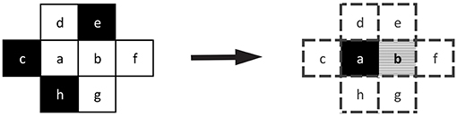
Figure 6. An example transition for pair ab. Sites c through h are their nearest neighbors. (Left) At the beginning of the update step, the pair ab has the configuration [00], i.e., both are inactive, while three neighbors are active. (Right) At the end of the update step, the pair ab has the new configuration [11], via self-activation for site a and via recruitment for site b.

The neighborhood configuration χ^* on the left shows the states at the beginning of an update step. Sites a, b, d, f, and g are inactive, and sites c, e, and h are active. The ab pair within χ^* has the state configuration [00]. The configuration on the right is a possible outcome at the end of the update step; in this case the pair has the state configuration [11]. Site a has self-activated, which can occur with probability α. Site b has activated via recruitment, which can occur with probability R(2, 1); the recruitment could have been induced either by its pair-neighbor a, or by one of the two non-pair neighbors f or g which had previously been inactive. (Note that the non-pair neighbor e could not have contributed to the recruitment, since it began the update step as active and subsequently would have been refractory).

Combining these observations, we have that the probability that this particular local neighborhood χ^* will produce this particular subtype pair (a self-activated and b recruited) is given by αR(2, 1).

Continuing this reasoning, we can now write down the production probabilities for the other three possible subtypes of [11] pairs:

$\begin{array}{ll}a\text{ and }b\text{ both self-activate}\hfill & {\alpha }^2\hfill \\ a\text{ is recruited},b\text{ self-activates}\hfill & R(1,1)\alpha \hfill \\ a\text{ and }b\text{ are both recruited}\hfill & R(1,0)R(2,0)\hfill \end{array}$

After adding together the probabilities for all subtypes, the total probability P[11∣χ^*] of this particular local neighborhood χ^* producing a pair of double activations [11] through whatever pathway is P[11 ∣ χ^*] = α² + αR(2, 1) + R(1, 1)α + R(1, 0)R(2, 0).

Note that this calculation needs to be repeated for each χ in order to complete the sum in the difference equation for P_t+1[11] (Equation 2), although we can reduce the computational load by taking symmetries into account (as indicated by the symmetry multipliers in Figure 5).

Having computed P_t+1[11], we must compute another term, say P_t+1[10], in a similar manner. (The remaining two terms P_t+1[01] and P_t+1[00] can be inferred via the symmetry assumption and the Law of Total Probability).

4.5. Computational Notes

Before moving on, we stop to consider some computational aspects. To advance one update step, the difference equations (Equation 2) requires a summation over 256 configurations of χ. Each iteration of the neighborhood function P_t[χ] requires a series of 11 multiplications and one division, plus sufficient additions to compute the marginal sums for the single-site probabilities. Importantly, the production function P [ab∣χ] is time-independent, and therefore can be pre-computed once and stored as the 4 × 256 matrix M. We also note that by the symmetry assumption and the Law of Total Probability, we can infer the updated value for two of the four P_t+1[ab].

Let $p={\left[\begin{array}{cccc}P[00]& P[01]& P[10]& P[11]\end{array}\right]}^T$ be the column vector of pair probabilities. We can then efficiently rewrite the difference equations in matrix-vector product form:

$p_{t+1}=M\pi \left(p_t\right)$

where π (p_t) is the neighborhood function which accepts the length-4 column vector p_t as input, and returns a length-256 column vector as output. Implementing these calculations on a system optimized for matrix operations is an efficient choice.

5. Quartet Approximation

With the machinery developed for the pair approximation in hand, we are now ready to extend the analysis to use of 2 × 2 blocks known as quartets (Figure 7). A quartet is a second-order structure, since it contains “neighbors of neighbors” (e.g., sites a and d). The main challenge in using quartets is combinatorial in nature; there are 2⁴ = 16 possible configurations for a quartet $\left[\begin{array}{cc}a& b\\ c& d\end{array}\right],$ and 2¹² = 4096 unique configurations for the associated neighborhood χ.

FIGURE 7

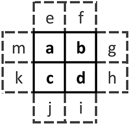
Figure 7. Template for the 2 × 2 quartet abcd and its eight nearest neighbors e through m. Each letter can take on the value 0 or 1.

Similar to the pair approximations, the quartet probabilities satisfy ${\displaystyle {\sum }_{a,b,c,d}P\left[\begin{array}{cc}a& b\\ c& d\end{array}\right]=1,}$ and we will make use of the marginal sum $P\left[ab\right]=\sum _{c,d}P\left[\begin{array}{cc}a& b\\ c& d\end{array}\right]$. We will again assume that the probabilities are symmetric with respect to spatial orientation, so that, for instance, $P\left[\begin{array}{cc}a& b\\ c& d\end{array}\right]=P\left[\begin{array}{cc}b& a\\ d& c\end{array}\right]$ = (reflection) and $P\left[\begin{array}{cc}a& b\\ c& d\end{array}\right]=P\left[\begin{array}{cc}c& a\\ d& b\end{array}\right]$ (rotation). In all, there are up to eight unique orientations for a given 2 × 2 structure.

The corresponding 16 difference equations are specified by

$\begin{array}{ll}{P}_{t+1}\left[\begin{array}{cc}a& b\\ c& d\end{array}\right]={\displaystyle \sum _{\chi }P}\left[\begin{array}{cc}a& b\\ c& d\end{array}\mid \chi \right]P_t[\chi ].& (4)\end{array}$

However, by invoking rotation and reflection symmetry, we need explicitly compute the updates only for the six equivalence classes for the quartet $\left[\begin{array}{cc}a& b\\ c& d\end{array}\right]$ (see Figure 8 for the six classes).

FIGURE 8

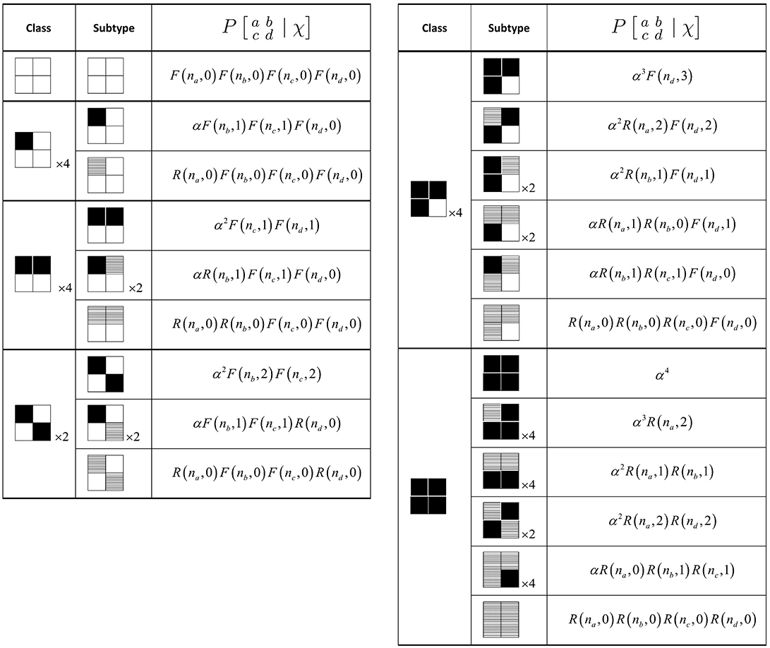
Figure 8. Production probability calculations for the quartet configurations. Site states are inactive (white), self-activated (black), or recruited (hatched). Functions R(n, j) and F(n, j) are as defined in the text. The available neighbor counts n_a through n_d are determined for each specific configuration of χ. The symmetry multipliers apply either to an entire class or a single subtype.

5.1. Computing the Neighborhood and Production Functions

The neighborhood structure in Figure 7 is fourth-order, and its joint probability must be approximated with second-order quartet probabilities. Using a similar method as with the pair approximation, we cover the neighborhood with 2 × 2 quartets to produce the neighborhood function

$\begin{array}{ll}P[\chi ]=P\left[\begin{array}{c}ef\\ mabg\\ kcdh\\ ji\end{array}\right]\approx \frac{P\left[\begin{array}{cc}m& a\\ k& c\end{array}\right]P\left[\begin{array}{cc}a& b\\ c& d\end{array}\right]P\left[\begin{array}{cc}b& g\\ d& h\end{array}\right]P\left[\begin{array}{cc}e& f\\ a& b\end{array}\right]P\left[\begin{array}{cc}c& d\\ j& i\end{array}\right]}{P[ac]P[bd]P[ab]P[cd]}.& (5)\end{array}$

Because the quartet probabilities are now the basic unit of computation, the pair probabilities in the denominator of Equation (5) must be computed as marginal sums.

Computation of the production function $P\left[\begin{array}{cc}a& b\\ c& d\end{array}\mid \chi \right]$ proceeds in the same manner as for the pair model, by enumerating the six classes for the quartet, and the number of subtypes representing the unique ways each quartet can be produced. The number of classes and subtypes, and the corresponding probability calculations, are summarized in Figure 8. Note that symmetry multipliers are specified to account for the number of ways in which a class (or a subtype) can be rotated or reflected. Once we have both the production and neighborhood functions, the difference equations in Equation (4) can be stepped forward.

6. Results for Approximation Methods

Plots of the observed and predicted amplitude A and clustering coefficient Q are given in Figure 9 (as a function of γ) and Figure 10 (as a comprehensive “heatmap” over the entire two-parameter α-γ space), allowing us to compare the performance of the three approximations (mean-field, pair, and quartet) against the PCA simulation results.

FIGURE 9

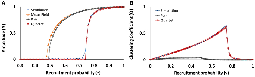
Figure 9. Amplitude coefficient A (A) and clustering coefficient Q (B) as a function of recruitment probability γ, for self-activation probability α held at 0.80. Values measured at the end of 500,000 steps, for numerical simulations and for mean-field, pair, and quartet approximations. The clustering coefficient cannot be calculated with the mean-field approximation.

FIGURE 10

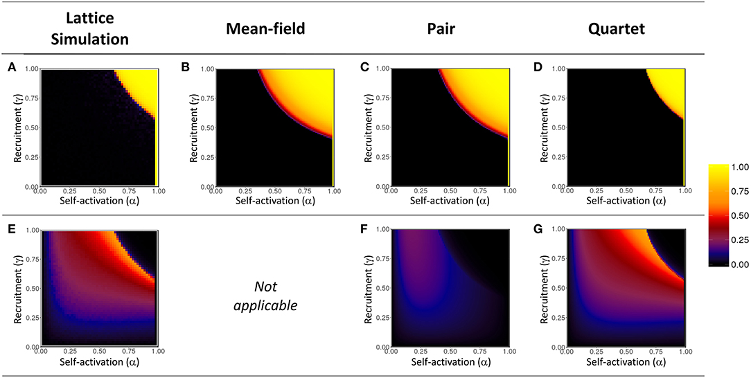
Figure 10. Heatmap visualization of amplitude coefficient A (top row, A–D), and clustering coefficient Q (bottom row, E–G), in α-γ parameter space. Values measured at the end of 500,000 steps, for numerical simulations and for mean-field, pair, and quartet approximations. The narrow vertical band of maximum amplitude (A ≈ 1) is the trivial case at α = 1 wherein the entire lattice oscillates in unison. The clustering coefficient cannot be calculated for the mean-field approximation. The color scale applies to both A and Q; rare negative values of Q were very near zero and are represented as such in the plot.

Amplitude. The lattice simulations reveal a well-defined window (where α and γ are both large) in which periodicity is present; outside the boundary of this window, the ensemble activation fraction settles into a non-oscillatory state. The threshold for onset of periodicity is fairly sharp. We also note that the location of the threshold is dependent on both α and γ, so that no single value of either parameter serves as a constant threshold. The shape and location of the threshold are replicated very well by the quartet approximation. On the other hand, the mean-field and pair approximations both show a much more gradual transition to periodic behavior beginning at a much smaller value of γ ≈ 0.46 (Figure 9A), as compared to the simulation results, and the periodic window is much larger (Figures 10B,C).

Spatial clustering. The spatial clustering coefficient show an excellent match between the simulation results and the values predicted by the quartet approximation. Clustering increases smoothly and gradually as α and γ are increased until the threshold of the periodicity region is reached. (Recall that, by design, Q will be near zero when A is near one; hence we observe the sudden loss of clustering as periodicity emerges.) The relationship of Q to the two probability parameters appears to be slightly asymmetrical, such that clustering is more prevalent for the region where γ > α. The pair approximation incorrectly predicts that only weak clustering (Q < 0.25) will occur, while the quartet approximation correctly captures the presence of more pronounced clustering (Q > 0.50) for a selected region near the threshold in α-γ space.

Quartet distributions. In Figure 11 we more closely examine the probability distribution across the six quartet classes, for α fixed at 0.80, and selected values of the recruitment probability γ (equal to those chosen previously in Figure 3). The activation fractions f (determined by computing the single-site probability P[1]) as well as the spatial clustering coefficients Q are a close match to those obtained from the simulations (compare results to Figure 3). From γ = 0.25 to γ = 0.74 we can clearly see that as Q increases, the class distribution shifts toward the two classes that are completely “empty” (all sites inactive) or “full” (all sites active), consistent with the fact that in a lattice with high spatial correlation, randomly-sampled quartets are more likely to be found in those two configurations, while the mixed-state configurations (in particular, the “checkerboard” quartet) are less likely as Q increases.

FIGURE 11

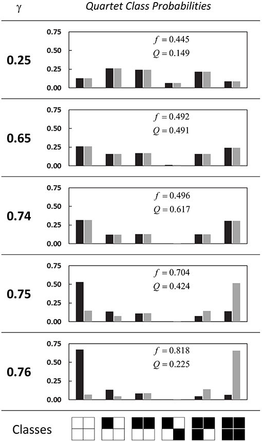
Figure 11. Probability distributions for the six quartet classes. Each panel is for a different value of the recruitment probability γ, and vertical axes are the class probabilities. Each pair of black-gray bars is the probability for two consecutive timesteps at t = 500,000 for that class. Also given are the single-site probabilities f and clustering coefficients Q for the second timestep. In all cases α is held at 0.80.

We can also observe the onset of periodicity around the threshold value of γ = 0.75, and the corresponding divergence between class probabilities on consecutive beats (the black and gray bars in the figure), so that the empty class and full class exchange roles as the dominant class. The first quartet class (the “empty” class) is prevalent on the first beat and rare on the second beat; the pattern is reversed for the last quartet class (the “full” class). The alternation pattern is apparent to a lesser degree in the second and fifth classes (containing, respectively, one and three active sites).

6.1. Computing Time

Computing times were compared for the simulation and approximation methods (Figure 12), using as the basis of comparison a standardized task of generating the data for the “heatmaps” in Figure 10. The lattice simulations required the most amount of time, 11,165 core-hours, which is equivalent to 43.6 clock hours on a 256-core cluster. As anticipated, the time required for the mean-field approximation, which involves the update of only a single difference equation (Equation 1), is almost negligible in comparison to the lattice simulation. Although the pair approximation method nominally requires the update of only one more difference equation, those updates involve the additional work of evaluating the neighborhood function (Equation 3) 16 times (once for each neighborhood configuration χ) on each update step. The quartet method requires the update of five difference equations and 4096 neighborhood configurations (Equation 5), and while the resulting computation time is almost 24 times as long as for the pair method, it is still only about one-twentieth (1/20) of the time required by the full simulation, a substantial savings.

FIGURE 12

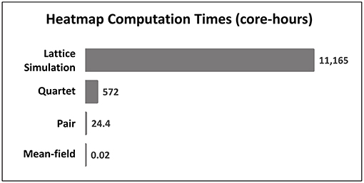
Figure 12. Computation times, measured in CPU core-hours, required to generated the “heatmaps” in Figure 10 for each method. Each bar represents the total computational work required to run the respective model for 500,000 update steps, repeatedly for 10,000 parameter combinations. Note that times are “real CPU” times for a single-core process, and do not include any additional overhead time which may have been incurred by the operating system or job scheduling manager.

7. Discussion

In this study we found that the moment-closure technique using quartet approximation provides a very good prediction of several macroscopic quantities (alternation in activation fraction, and spatial clustering) of a probabilistic cellular automata model with two-stage update rules. As with all closure methods, the second-order quartet approximation vastly reduces the complexity of the original PCA simulation, so that such macroscopic variables can be approached in a more abstract manner; however it does not reduce the complexity so much that it completely discards all information about the spatial interactions and subsequent pattern formation, as happens with the lowest-order mean-field approximation. The increased computational cost associated with a higher-order closure is still an order of magnitude smaller than the original simulations.

A particular challenge with the PCA model in the present study is the two-stage, or split-step, update rules, wherein each stage is applied sequentially within a single overall update step. The resulting large number of possible configurations that can result after each update step provides a richness to both the dynamics of the model behavior and the analysis required in applying the approximation methods. Even the relatively simple set of update rules used in the present model results in a combinatorially complex set of possible configurations that must be accounted for if a quantitatively accurate approximation is to be achieved. In this study we demonstrate a method by which we can systematically enumerate the complete set of possible configurations.

The unique nature of the split-step update rules also means that this particular PCA model may not fit the usual classifications reserved for probabilistic cellular automata, and is more reminiscent of the classic lattice gas automata [23]. It may be possible, however cumbersome, to recast the update rules so that they may be expressed as a single unified set not requiring the split-step paradigm. Alternatively, the model might be reformulated as a coupled set of two lattices; each lattice would correspond to one of the two half-steps of the update cycle.

By implementing a second-order approximation for this model, a framework has been established by which pattern formation dynamics might be formally studied. For instance, the third quartet class in Figure 11, in which a pair of active sites is next to a pair of inactive sites, could serve as a rudimentary “edge detector”, whose probability of occurrence is high when active sites are highly clustered and almost completely segregated from inactive sites (as might occur with striping or spotting patterns). The approaches for constructing both the neighborhood and production functions can be systematically generalized to larger neighborhood structures (for example, a 3-by-3 “nonet” involving fourth-order interactions) which could provide even more useful information regarding pattern dynamics, although at a considerable computational cost.

The combination of the three primary factors driving the dynamics of the PCA model (randomness, recruitment, and refractoriness) has been called the “3R model” [24] and has been used successfully to provide a detailed explanation for various physiological features of intracellular calcium release in cardiac myocytes, including calcium alternans. These three factors, although treated abstractly in this analysis, can be readily identified with real components in the cellular physiology, offering the chance to develop new experimental targets in medical research. This PCA approach could be adapted to any system with these three factors in order to model phenomena in other areas of physiology (for instance, muscle or neural tissue), ecology, or physics that arise from large systems of coupled, randomly excitable elements with similar spatial interactions.

In contrast with the present analysis, the original development of this PCA model [11, 12] treated refractoriness as an additional probabilistic variable, which is more consistent with the known physiology of calcium release, wherein the potential recovery of the CRUs has a complex dependence on pacing rate and other factors (see, e.g., [25]). In this analysis we have essentially assumed that CRUs will be refractory with probability 1, but this could be modified in future work. We have also yet to explore the effects of differing lattice topology (e.g., non-square lattice dimensions or more complex connectivity to neighboring units) which would also be more physiologically realistic.

In the heatmap plots of the amplitude (Figure 10), the threshold for the onset of periodicity appears to be a relatively smooth curve in α-γ parameter space. The location of this threshold (or bifurcation) can be derived exactly [11] via a linear stability analysis in the mean-field approximation, however the functional form that is obtained is rather complicated and does not suggest a straightforward interpretation in terms of the underlying probabilistic parameters. We should not reasonably anticipate that applying the same linear stability analysis to the coupled difference equations for the pair and quartet methods would yield an expression any less complicated, although using the stability analysis to estimate the threshold curve numerically may very well be possible.

Author Contributions

The author confirms being the sole contributor of this work and has approved it for publication.

Conflict of Interest Statement

The author declares that the research was conducted in the absence of any commercial or financial relationships that could be construed as a potential conflict of interest.

References

1. Louis PY, Nardi FR. Probabilistic Cellular Automata: Theory, Applications and Future Perspectives, Vol. 27. Cham: Springer (2018).

Google Scholar

2. Kuehn C. Moment Closure—A Brief Review. Schöll E, Klapp SHL, Hövel P, editors. Cham: Springer International Publishing (2016). p. 253–71.

Google Scholar

3. Gutowitz HA, Victor JD, Knight BW. Local structure theory for cellular automata. Phys D Nonlinear Phenomena. (1987) 28:18–48. doi: 10.1016/0167-2789(87)90120-5

CrossRef Full Text | Google Scholar

4. ben Avraham D, Köhler J. Mean-field (n,m)-cluster approximation for lattice models. Phys Rev A. (1992) 45:8358–70. doi: 10.1103/PhysRevA.45.8358

PubMed Abstract | CrossRef Full Text | Google Scholar

5. Lion S. Moment equations in spatial evolutionary ecology. J Theor Biol. (2016) 405:46–57. doi: 10.1016/j.jtbi.2015.10.014

PubMed Abstract | CrossRef Full Text | Google Scholar

6. Satō K, Matsuda H, Sasaki A. Pathogen invasion and host extinction in lattice structured populations. J Math Biol. (1994) 32:251–68. doi: 10.1007/BF00163881

PubMed Abstract | CrossRef Full Text | Google Scholar

7. Pugliese E, Castellano C. Heterogeneous pair approximation for voter models on networks. Europhys Lett. (2009) 88:58004. doi: 10.1209/0295-5075/88/58004

CrossRef Full Text | Google Scholar

8. Hiebeler D. Stochastic spatial models: from simulations to mean field and local structure approximations. J Theor Biol. (1997) 187:307–19. doi: 10.1006/jtbi.1997.0422

CrossRef Full Text | Google Scholar

9. Hiebeler DE, Millett NE. Pair and triplet approximation of a spatial lattice population model with multiscale dispersal using Markov chains for estimating spatial autocorrelation. J Theor Biol. (2011) 279:74–82. doi: 10.1016/j.jtbi.2011.03.027

PubMed Abstract | CrossRef Full Text | Google Scholar

10. Petermann T, De Los Rios P. Cluster approximations for epidemic processes: a systematic description of correlations beyond the pair level. J Theor Biol. (2004) 229:1–11. doi: 10.1016/j.jtbi.2004.02.017

PubMed Abstract | CrossRef Full Text | Google Scholar

11. Rovetti R, Cui X, Garfinkel A, Weiss JN, Qu Z. Spark-induced sparks as a mechanism of intracellular calcium alternans in cardiac myocytes. Circ Res. (2010) 106:1582. doi: 10.1161/CIRCRESAHA.109.213975

PubMed Abstract | CrossRef Full Text | Google Scholar

12. Cui X, Rovetti RJ, Yang L, Garfinkel A, Weiss JN, Qu Z. Period-doubling bifurcation in an array of coupled stochastically excitable elements subjected to global periodic forcing. Phys Rev Lett. (2009) 103:044102. doi: 10.1103/PhysRevLett.103.044102

PubMed Abstract | CrossRef Full Text | Google Scholar

13. Nivala M, de Lange E, Rovetti R, Qu Z. Computational modeling and numerical methods for spatiotemporal calcium cycling in ventricular myocytes. Front Physiol. (2012) 3:114. doi: 10.3389/fphys.2012.00114

PubMed Abstract | CrossRef Full Text | Google Scholar

14. Franzini-Armstrong C, Protasi F, Ramesh V. Shape, size, and distribution of Ca(2+) release units and couplons in skeletal and cardiac muscles. Biophys J. (1999) 77:1528–39. doi: 10.1016/S0006-3495(99)77000-1

PubMed Abstract | CrossRef Full Text | Google Scholar

15. Chudin E, Goldhaber J, Garfinkel A, Weiss J, Kogan B. Intracellular Ca²+ dynamics and the stability of ventricular tachycardia. Biophys J. (1999) 77:2930–41. doi: 10.1016/S0006-3495(99)77126-2

CrossRef Full Text | Google Scholar

16. Qu Z, Nivala M, Weiss JN. Calcium alternans in cardiac myocytes: order from disorder. J Mol Cell Cardiol. (2013) 58:100–9. doi: 10.1016/j.yjmcc.2012.10.007

PubMed Abstract | CrossRef Full Text | Google Scholar

17. Weber CR, Ginsburg KS, Philipson KD, Shannon TR, Bers DM. Allosteric regulation of Na/Ca exchange current by cytosolic Ca in intact cardiac myocytes. J Gen Physiol. (2001) 117:119–31. doi: 10.1085/jgp.117.2.119

PubMed Abstract | CrossRef Full Text | Google Scholar

18. Kockskamper J, Blatter LA. Subcellular Ca²+ alternans represents a novel mechanism for the generation of arrhythmogenic Ca²+ waves in cat atrial myocytes. J Physiol. (2002) 545:65–79. doi: 10.1113/jphysiol.2002.025502

PubMed Abstract | CrossRef Full Text | Google Scholar

19. Tian Q, Kaestner L, Lipp P. Noise-free visualization of microscopic calcium signaling by pixel-wise fitting. Circ Res. (2012) 111:17–27. doi: 10.1161/CIRCRESAHA.112.266403

PubMed Abstract | CrossRef Full Text | Google Scholar

20. Sanderson C, Curtin R. Armadillo: a template-based C++ library for linear algebra. J Open Sour Softw. (2016) 1:26. doi: 10.21105/joss.00026

CrossRef Full Text | Google Scholar

21. Marsaglia G. Xorshift rngs. J Stat Softw. (2003) 8:1–6. doi: 10.18637/jss.v008.i14

CrossRef Full Text | Google Scholar

22. Filipe JAN, Gibson GJ. Comparing approximations to spatio-temporal models for epidemics with local spread. Bull Math Biol. (2001) 63:603–24. doi: 10.1006/bulm.2001.0234

PubMed Abstract | CrossRef Full Text | Google Scholar

23. Wolf-Gladrow DA. Lattice-Gas Cellular Automata and Lattice Boltzmann Models: An Introduction. Berlin: Springer (2004).

Google Scholar

24. Qu Z, Liu MB, Nivala M. A unified theory of calcium alternans in ventricular myocytes. Sci Rep. (2016) 6:35625. doi: 10.1038/srep35625

PubMed Abstract | CrossRef Full Text | Google Scholar

25. Sobie EA, Song LS, Lederer W. Restitution of Ca²+ release and vulnerability to arrhythmias. J Cardiovasc Electrophysiol. (2006) 17:S64–70. doi: 10.1111/j.1540-8167.2006.00385.x

CrossRef Full Text | Google Scholar