Happy Catastrophe: Recent Progress in Analysis and Exploitation of Elastic Instability

1. Introduction

Bernard Budiansky famously used to say “everybody loves a buckling problem” [1, 2] and this resonates today in a number of significant ways. First, it reflects that buckling is a process of instability, and instabilities have always held a macabre fascination for children and adults alike. From the collapse of a pile of bricks to the deliberate demolition of buildings or the catastrophic failures of large urban areas in the aftermath of a natural disaster, instabilities hold a central place in human experience and consciousness. But there is a newer, more modern, context—that structural instabilities can also be harnessed for the greater good. See, for example, the recent paper by Reis [3] who coined the phrase buckliphilia for the exploitation of instability in counterpoint to buckliphobia, the safety-conscious avoidance of collapse.

The purpose here is to review modern developments in the theory and analysis of buckling instabilities, both in the work of the present authors and by others. In the process, we draw particular attention to new techniques of analysis—often applied to classical thorny buckliphobic problems—and highlight potential areas of buckliphilic exploitation. We place particular emphasis on the interplay between analytical, numerical and experimental techniques, showing how we pick our way through a plethora of unstable post-buckling equilibrium states, to focus on practically relevant solutions.

With its origins in singularity, or catastrophe, theory [4, 5], the non-linear analysis of structural buckling can be cast in the framework of static bifurcation theory. Broadly speaking, the instability of a trivial, unbuckled state, upon varying an external load parameter, falls into one of three categories: supercritical, subcritical or transcritical; see Figure 1. The former is sometimes called a safe bifurcation because, as shown in panel (A), the post-buckled path emerges smoothly out of the unbuckled equilibrium path, and hence stability can be safely tracked under slow variation of the applied load. In contrast, subcritical bifurcations, as seen in panel (B), have been termed dangerous [6], because the structure would irreversibly jump to a post-buckled state (not shown) that is a long way from the trivial one. Such jumps in elastic structures tend to give rise to energy loss, accompanied by a significant “bang,” and often lead to permanent non-elastic deformation or collapse. Transcritical instabilities (C) lie somewhere in between and are often associated with a loss of reflection symmetry. There is an extensive literature on understanding and classifying buckling instabilities, see for example Thompson and Hunt [7] and references therein. This paper shall concern instabilities that lead to large irreversible jumps.

FIGURE 1

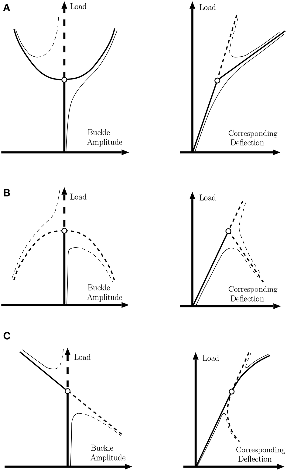
Figure 1. (A) Supercritical, (B) subcritical, and (C) transcritical buckling instabilities and their unfolding in the presence of small symmetry-breaking effects. Heavy lines: perfect system. Light lines: imperfect system. Solid lines: stable. Broken lines: unstable under controlled load.

Subcritical bifurcations, exemplified by the classic responses of thin elastic shells, are known to carry distinctive features, such as the likelihood of extreme imperfection-sensitivity and wide experimental scatter, and certainly merit a general overview. The canonical example is that of the axially-loaded cylindrical shell, of interest to rocket designers, aircraft and storage tank manufacturers, as well as in the construction of buffers to absorb mechanical energy. Here, instability under realistic conditions occurs significantly below the critical load of the system as determined from linear stability analysis of the perfect problem, absent from imperfections.

One approach to deal with such imperfection-sensitivity is through stochastic methods. Eliashakoff, Arbocz, and others pioneered developments, such as the international databank of imperfections (see [8, 9]) and references therein. While such methods appeal at one level, from a modeling point of view there is also significant sensitivity to the precision of the chosen numerical method, and useful analyses typically require many Monte Carlo realizations. Also, from a practical perspective, estimating a safety margin of a particular specimen would necessitate comprehensive imaging and analysis of all its imperfections. Unfortunately for modern, lightweight composite structures, such imperfections often occur beneath the surface layer and are hard to characterize in practice. There has therefore long been a search for a lower-bound criterion below which a violently subcritical structure, such as a cylindrical shell cannot buckle. One such phenomenological idea is that of a “reduced stiffness” approach [10], but such simple design formulae still require a full understanding of the non-linear elastic equilibrium states of the shell.

Methods based on sensitivity to perturbations have received a recent resurgence of interest inspired by theories of critical transitions in fluid dynamics, see for example [11, 12]. The focus in these works is sensitivity not to imperfection but to dynamic shocks; how large a dynamic perturbation in the form of a small tap or localized impact would be needed to induce buckling. It is not clear yet whether such ideas represent a realistic prospect for a practical non-destructive test for a particular specimen. Nevertheless, we shall argue in section 5 below that small localized shocks can allow engineers to explore the critical mountain pass unstable equilibrium that provides the route to buckling.

Fundamentally, this paper takes a deterministic rather than stochastic point of view. Starting with the perturbation methods introduced by the Dutch engineer [13], there is a rich tradition of using pseudo arc-length continuation to track unstable post-buckling solutions emerging from classical bifurcation points [14–18]. Supplemented by energy landscape considerations providing information on stability, these methods can be interpreted fundamentally as implicit analytical approaches to studying equilibrium solutions and their buckling paths. On the other hand, stochastic formulations, primarily explicit, after the introduction of quasi-realistic imperfection types and shapes and often employing Monte Carlo techniques, can be used to track expected dynamical behavior for particular specimens (see e.g., [19, 20]). Clearly, both approaches carry inherent advantages and disadvantages, and should be regarded as complementary.

A key idea is that the perfect problem, devoid of imperfections or shocks, can give theoretical and practical insight into how structures buckle subcritically. We shall emphasize the significance of the Maxwell load, the level at the fundamental and periodic buckle patterns have the same energy (see e.g., [21]) and section 4 below. Nearby spatially localized equilibria are energetically preferable. But to find such states, we need to overcome an energy barrier, in the form of snaking or concertina pattern of unstable states connected by sequences of folds. Numerically, these patterns can be captured using pseudo-arclength continuation, going back to Riks [22]. But how can we embed such a methodology in modern finite-element analyses? How can one access such unstable paths in an experiment? What is the best approach to understanding energy barriers? These are the questions this paper seeks to answer. We shall also keep in mind the perspective [3] that buckling instabilities, rather than to be avoided at all costs, can, in principle, be beneficial happy catastrophes.

The rest of this paper is outlined as follows. Section 2 gives a brief overview of non-linear post-buckling analysis of subcritical problems, starting from the pivotal work of Koiter, and including some general comments on analytical perturbation methods. A motivating simple pin-jointed “knee” model is presented as well as the classical problem of the axially loaded cylindrical shell. Section 3 surveys recent progress in computational path-following methods applied directly to a finite element representation to compute stable and unstable paths, with illustrations for a simple snap-through structure as well as the more complex cylindrical shell. Section 4 then considers computational energy-based methods that are able to identify Maxwell loads and mountain-pass solutions, again with reference to the cylindrical shell. Section 5 considers emerging experimental ideas to implement the numerical methods from the previous sections, via carefully controlled laboratory procedures. Section 6 surveys three examples, at different length-scales and from distinct engineering domains, that attempt to exploit subcritical buckling instabilities: prestressed stayed columns, adaptive aeroelastic structures, and a structural model for auxetic materials. Finally, section 7 draws conclusions and suggests avenues for future work.

2. Large Amplitude Post-buckling Analysis

Before the advent of modern computer-based methods, non-linear post-buckling of elastic structures was largely dealt with by systematic asymptotic analysis; i.e., perturbation procedures based on Taylor expansions about the critical bifurcation point [7, 23]. The pioneer of this field was Warner T. Koiter (1914–1997), beginning with his PhD thesis, completed during the Second World War [13]. Local perturbation analysis can be highly instructive in highlighting fundamental properties like underlying symmetries and symmetry-breaking, yet its range of validity typically is limited. This observation is by no means new. Koiter, for example, in discussing the buckling of a spherical shell under external pressure in 1969 [24], states:

“In the problem of the spherical shell under external pressure the systematic perturbation procedure is only valid in a range of load factors within a fraction of the order h/R of the critical load, and for deflections of the order (h/R)^1/2 times the shell thickness. It follows that the systematic perturbation procedure at the critical point has little, if any, practical significance for the present problem.”

Here h represents the shell thickness and R the radius. He went on to suggest the following:

“A far more powerful method of achieving a second approximation to the post-buckling behavior was also developed already in our earlier work [13, section 38]. It consists of an evaluation of the quartic terms in the energy expression not at the critical load itself, but at the actual value of the load factor under consideration.”

The reference is of course to his thesis [13], which did not appear in English until 1967 and was never published in the open literature. Koiter was a deeply humble man.

In more recent years Koiter's ideas have been supplemented by other asymptotic techniques, such as expansions at the so-called Maxwell load [25] and pseudo arc-length continuation which will be explained in section 3 below. Throughout this article we will apply our ideas to the recurring infinite-degree-of-freedom example of the axially-compressed cylindrical shell. But first, let us introduce a simple single degree-of-freedom example.

2.1. A Simple Motivating Example

Consider the simple mechanical model of Figure 2. A linear spring k is placed in-line with a “knee” comprising two finite-length rigid links hinged with a rotational spring, and compressed by an axial force P as shown. The rotational spring can take various characteristics—elastic, rigid-plastic or elasto-plastic, as shown in the insets. It is also assumed that the arms can pass through one another without restriction.

FIGURE 2

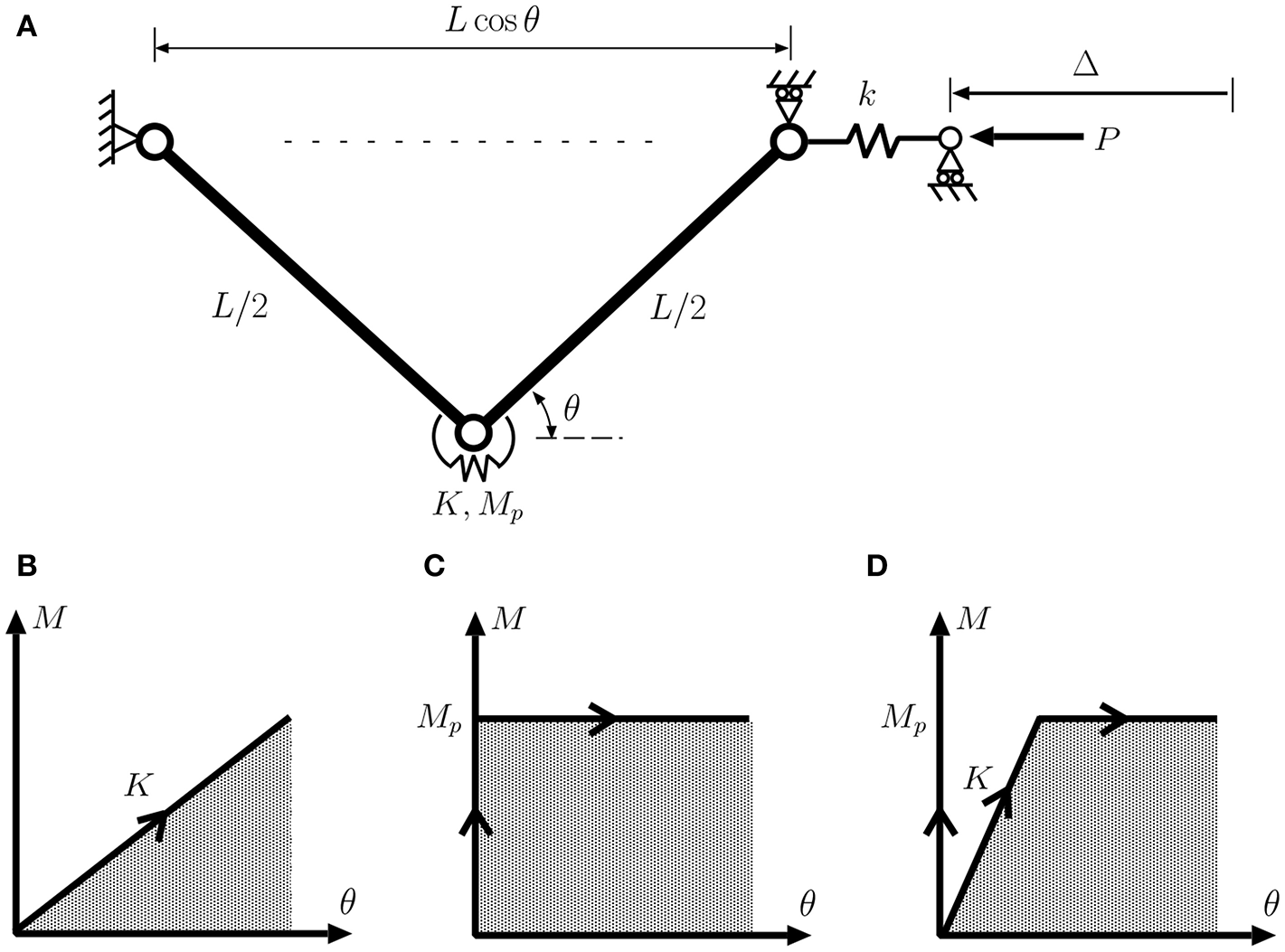
Figure 2. (A) Schematic of a simple knee model. (B–D) Load-deflection diagrams for the case of (B) an elastic rotational spring, (C) rigid–plastic rotational spring and (D) elasto-plastic rotational spring.

The system has two degrees-of-freedom, with associated generalized coordinates Δ and θ that respectively describe in-line displacement and rotation of the rigid link elements. It has three distinct possibilities for equilibrium. First, we have the simplest state in which the rotational spring does no work and the in-line spring simply squashes to give a fundamental equilibrium path describing the pre-buckling state:

$\begin{array}{ll}P=k\Delta .& (1)\end{array}$

Second, under the condition that the knee rotation θ continues to grow in the positive sense, the potential energy function for the post-buckling response is either

$\begin{array}{l}V=\frac{1}{2}K{(2\theta )}^2+\frac{1}{2}k{\left[\Delta -L(1-cos\theta )\right]}^2-P\Delta ,\end{array}$

when the rotational spring is elastic with rotational stiffness K, or

$\begin{array}{l}V=2M_p\theta +\frac{1}{2}k{\left[\Delta -L(1-cos\theta )\right]}^2-P\Delta ,\end{array}$

if it has passed its limiting plastic moment M_p. In each case, the first two terms are the strain energies in the rotational and in-line springs, respectively; the final subtracted term is the work done by the dead load P. When the rotational spring is in the plastic state, its energy contribution can be seen as quasi-strain energy, i.e., the work done in moving the joint through positive rotation, without necessarily being able to release this work if the rotation is reversed. Responses are then readily obtained in closed form from the two equilibrium equations ∂V/∂θ = 0 and ∂V/∂Δ = 0.

The fundamental and post-buckling paths are plotted in Figure 3. for the three possibilities of Figure 2. There are several points worthy of note. For the elastic system of Figure 2A the initially-stable pure-squash fundamental equilibrium state reaches a supercritical bifurcation point B where it becomes unstable, whereupon one branch of the stable post-buckling path is then followed. Post-buckling analysis of this type of behavior responds well to the perturbation method [7].

FIGURE 3

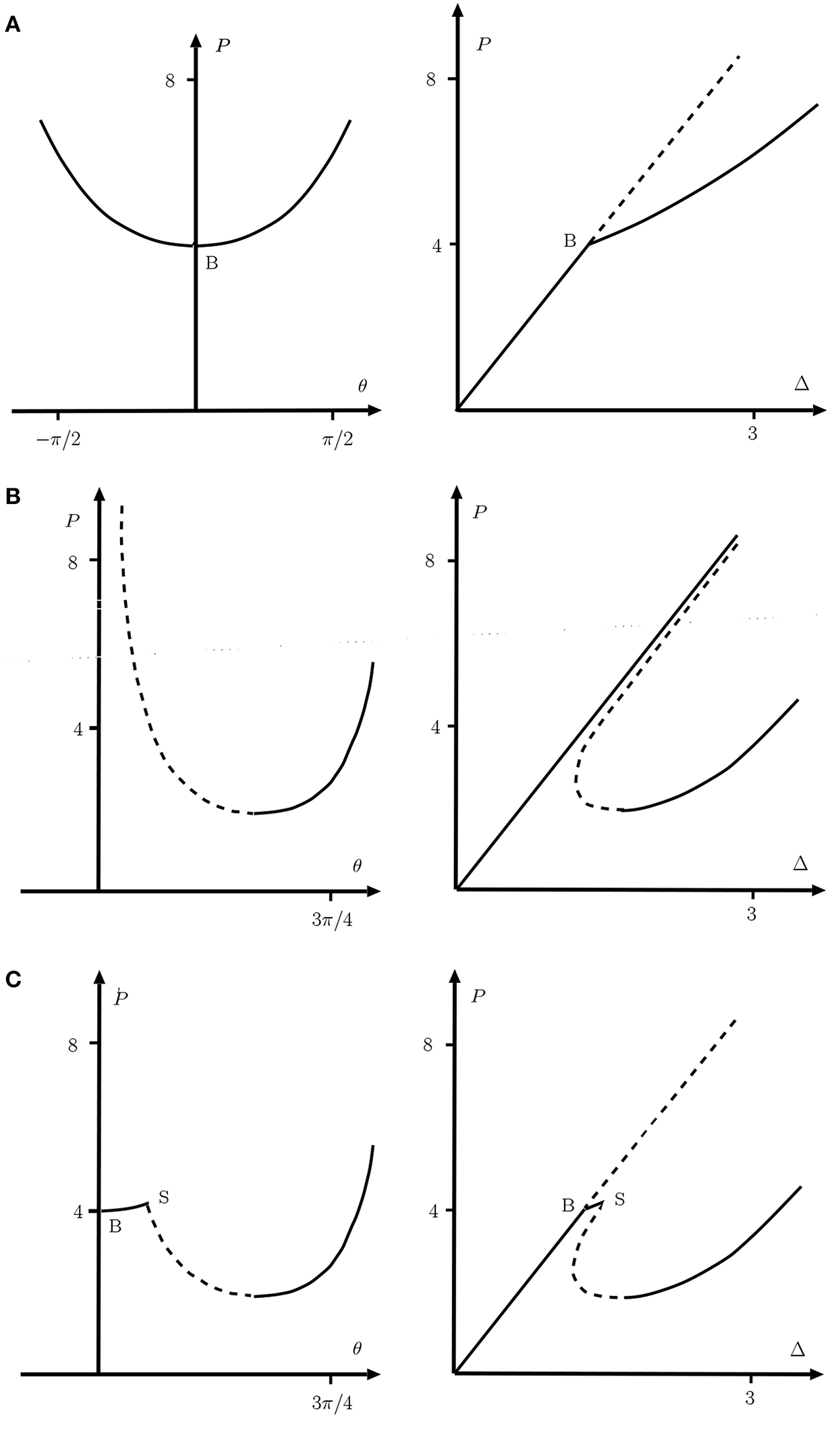
Figure 3. Responses of the knee models of Figure 2 for the parameter values L = 1, k = 3, K = 1, and M_p = 1. (Left) Load vs. θ. (Right) Load vs. end-shortening. (A) Elastic joint of Figure 2B. (B) Rigid-plastic joint of Figure 2C. (C) Elasto-plastic joint of Figure 2D. Unstable paths under controlled load are shown as broken lines.

The rigid-plastic system on the other hand has no bifurcation point, and this highlights one of the key issues to be addressed in this paper. Over much of the range, the fundamental and post-buckling paths, although being relatively well-separated in the P−θ plot, lie close to one another in the P−Δ diagram. Moreover, although the paths approach each other asymptotically, they never meet; the bifurcation exists only at infinite load. Yet when the load is high, buckling could certainly be triggered by small imperfections or fluctuations. So the real problem becomes to determine a practical range of loads over which the system can be assumed to be relatively safe from instability. Another point to note in this case is that although the buckled path represents pure plastic behavior with zero stiffness, there remains an effective stiffness on this path beyond its minimum load point, once the arms have passed through vertical. This stiffness is due to geometric effects (deflection perpendicular to the load remaining constrained). A number of circumstances are known where such geometrically non-linear, infinite-buckling-load problems arise in practice, for instance the buckling of railway tracks in heatwave conditions [26], and kink-banding of layered materials [27]. A major theme here is to review techniques for obtaining ball-park estimates for effective buckling loads and post-buckling information for such problems.

The bifurcation point is restored for the elasto-plastic system as shown in the bottom row of panels in Figure 3, where the behavior follows the purely elastic response of the top panels until the rotational moment reaches its plastic limit, whereupon it switches to the rigid-plastic response of the middle row. The absence of a first bifurcation point is avoided, but an effective secondary bifurcation point S also needs to be negotiated. As with many interactive buckling problems there is the danger that the continuation of the elastic path remains as a possible equilibrium solution. This simple example emphasizes that modern path-following computational methods need to be constantly vigilant in checking for further instability points and bifurcations as they track along an equilibrium path.

2.2. The Axially-Compressed Cylindrical Shell

Much has been written on the classical problem of the buckling of an axially loaded cylindrical shell (see e.g., [2, 28]) and references therein. It carries all the hallmarks of a classical subcritical buckling problem, in particular its notorious sensitivity to imperfections. Its apparent simplicity, yet underlying complexity, has ignited significant academic dueling over the course of the last century (cf. different “resolutions” of the “paradox” by Zhu et al. [29] and Elishakoff [30]), and caused design engineers many a headache.

It might seem strange in a forward-looking review paper to focus on such a problem, but with the modern impetus toward ever stronger and lighter structures and new materials, understanding the cylinder response remains a fundamental issue of continuing research. We will therefore use axially-compressed cylindrical shell buckling as the exemplar problem on which to illustrate the methodology reviewed in this paper.

When the fundamental deformation mode of a long, slender structure loses stability, it can either transition into a periodic buckling mode, spread equally over the domain, or a localized mode that is concentrated only over a portion of the domain. Such different kinds of buckle patterns were illustrated in the beautiful experimental and computational work of Yamaki [31]. It is well-known that localized post-buckling modes have a proclivity to develop in systems governed by subcritical bifurcations [32]. Moreover, Hunt and Lucena [33] showed that axially localized post-buckling modes exist for the axially compressed cylinder. This circumferential ring of an axially localized, diamond-shaped waveform can then undergo homoclinic snaking in the compressive loading parameter, leading to sequential ring formation along the length of the cylinder [34].

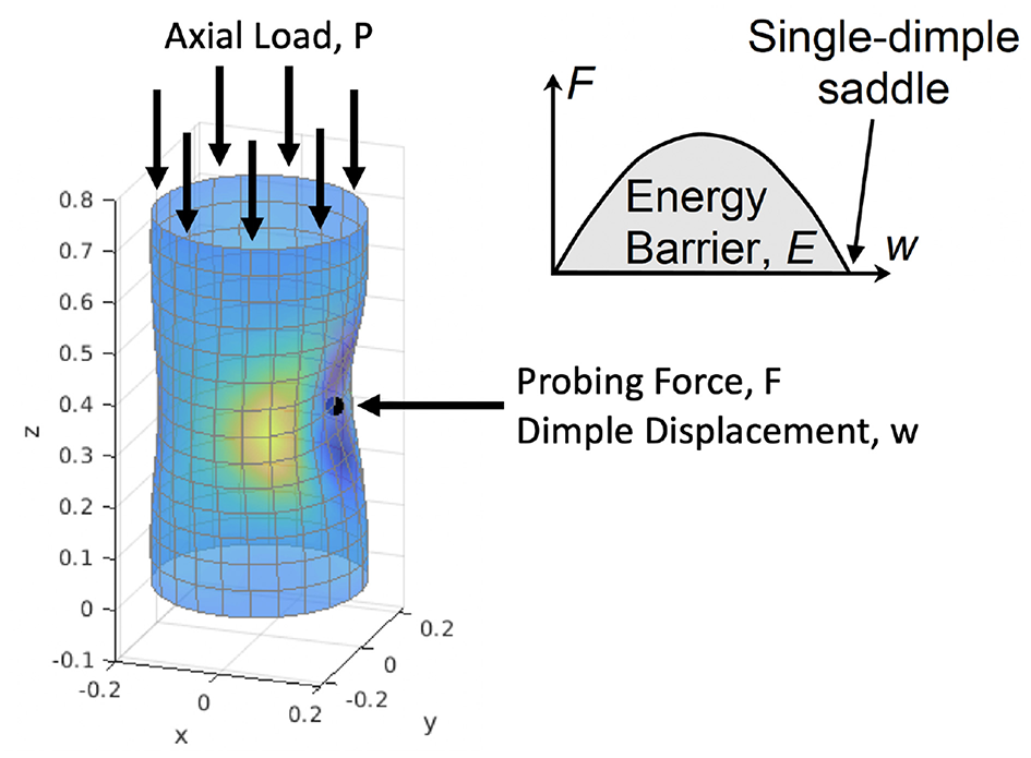
The work by Horák et al. [35] showed that an unstable equilibrium—localized axially and circumferentially—in the form of a single dimple is also possible (see Figure 4A). This state corresponds to the mountain-pass solution separating the stable pre-buckling and restabilized post-buckled states. The initial dimple, which can be found using the mountain pass algorithm of section 4, can undergo circumferential snaking, culminating in one ring of diamond-shaped buckles (see Figure 4B). This type of circumferentially-driven snaking is different from the axially-driven snaking described by Hunt et al. [34], where circumferentially-complete rings of buckles grow axially in a sequential manner.

FIGURE 4

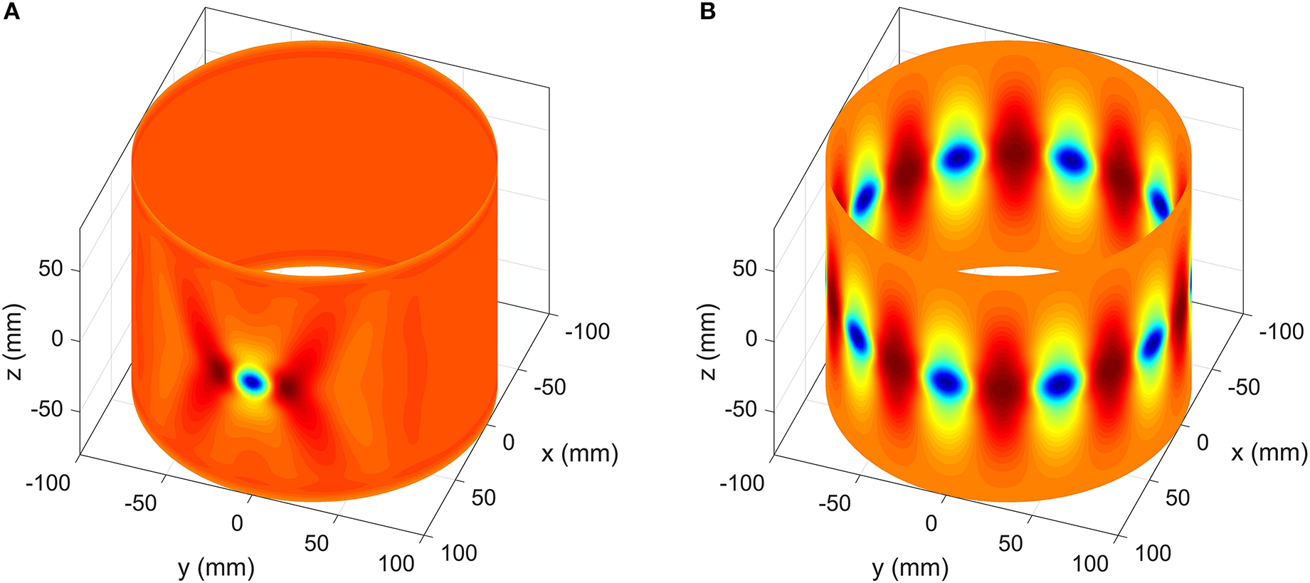
Figure 4. (A) An axially compressed cylinder features an unstable post-buckling equilibrium in the shape of a single inwards dimple, corresponding to the mountain-pass point between the stable pre-buckling and restabilized post-buckling regimes. (B) Through the process described in section 3 the single dimple can multiply circumferentially to form a single row of axially-localized buckles.

We shall continually return to the squashed cylinder problem throughout this study.

2.3. Post-buckling Analysis—A Post-Koiter Reflection

Another canonical shell buckling problem that has received a resurgence of interest due to the recent work of Hutchinson [36] is that of the spherical shell under uniform external pressure. That problem too exhibits violently subcritical bifurcation and shock-sensitivity. In an extended paper published in 1969 [24] writes

“An important result of Beaty's analysis [37] was that the numerical factor of the quartic term is much larger than the coefficient of the cubic term, indicating that the quartic term becomes already important for very small deflections in terms of the shell thickness, and that it is dominant over the cubic term for larger deflections. A similar evaluation of the quartic term in the energy expression at the critical load factor and for rotationally symmetric deformations was made independently by Walker [38], who also evaluated the next higher-order term, namely the quintic term, with an even larger numerical coefficient.”

He thus puts the poor performance of the perturbation method down to ever increasing influence of higher and higher-order terms—quartics larger than cubics, quintics more than quartics, and so on. This significant observation seems odd from the viewpoint of perturbation theory; using von Kármán–Donnell equations for the cylindrical shell [39] for example, a discrete formulation comprising doubly-periodic shapes generates energy terms only up to quartic level [7].

The need for higher-order terms can be explained through the process of elimination of passive coordinates, as espoused in the book by Thompson and Hunt [7]. Consider a conservative elastic structural system whose stable equilibrium configurations are described by minima of the energy function W(q_i, Λ), where {q_i} describes a set of n incremental generalized coordinates measured from a monotonically-increasing (fundamental) equilibrium path in loading parameter Λ. Suppose that n − m of the q_i are deemed passive (not actively involved in the buckling process). These passive terms are represented parametrically in terms of the remaining m active coordinates and loading parameter thus, q_α = q_α(q_j, Λ), where now 1 ≤ j ≤ m and m + 1 ≤ α ≤ n. A new energy function ${W}$(q_j, Λ), equal in value to the W-function, but written in terms of just the active coordinates and loading parameter, is introduced:

$\begin{array}{ll}{W}(q_i,\Lambda )\equiv W\left[q_j,q_{\alpha }(q_j,\Lambda ),\Lambda \right].& (2)\end{array}$

Differentiation using the chain rule then gives derivatives of ${W}$ in terms of W. Specifically, if W is diagonalized such that W_ij = 0 for i ≠ j, subscripts denoting partial differentiation with respect to the appropriate generalized coordinate, then derivatives up to cubic level pass over unchanged, but at quartic level we see contamination from lower-order derivatives. In particular,

$\begin{array}{ll}{{W}}_{1111}=W_{1111}-3{\displaystyle \sum _{\alpha =m+1}^n}\frac{W_{\alpha 11}^2}{W_{\alpha \alpha }}& (3)\end{array}$

for a significant quartic term (see [7] for more details). Similar contamination from lower derivatives likewise appears at quintic level and above, leading to a lack of convergence as described in the Koiter quote above.

The derivative W_αα appearing in the denominator of (3) is the so-called stability coefficient for the passive coordinate q_α, and would have equated to zero had the coordinate been active and directly involved in the buckling process, If critical loads tend to bunch together on the fundamental path, as occurs for both the axially-compressed cylinder and pressurized sphere discussed above, then contamination from higher-modes close to the critical point of interest can clearly be extreme.

Modal analysis in the form of spectral or pseudo-spectral numerical methods made a resurgence in the 1990s and 2000s, allowing numerical continuation (path-following) methods to scale to models with hundreds of degrees-of-freedom (see e.g., [21, 40]). Nowadays, with modern computers being able to cope easily with millions of degrees-of-freedom, because of its geometric versatility the finite element method is the preferred technique for solving complex problems in engineering mechanics. Results provided in the next section are therefore presented in a finite-element setting.

3. Numerical Path-Following for Subcritical Instabilities

In applied mathematics, methods for multi-parameter analysis, branch-switching and bifurcation tracking are well-established theoretically using the language of catastrophe (singularity) theory [41] and differentiable dynamical systems (see [42]), including in infinite dimensions [43]. Using the concept of pseudo-arclength continuation due to Keller [44] these methods have been implemented numerically and incorporated into a variety of numerical continuation software packages, such as AUTO [45]. Typically such formulations apply to systems governed by ordinary or partial differential equations. In structural mechanics, specialized arc-length techniques were developed for non-linear formulations by Riks [14] and Crisfield [15]. Classically, those studies tended to be restricted to a single parameter—the applied load. However, the formulation can easily be extended to the general setting, as described here.

Our formulation considers a discretized model of a quasi-statically evolving, conservative and elastic structure, where the internal forces, f(u), and tangential stiffness, K_T(u), are uniquely defined from the current displacements, u, by means of the first and second variations of the total potential energy. Here u may represent all the degrees-of-freedom of a simple system, or a large-scale reduction of an infinite-dimensional problem. We first present a general framework, then illustrate the results for a simple toggle frame, before discussing implications for the cylindrical shell problem.

3.1. The General Setting

Equilibrium is defined as a balance between internal and external forces acting on the structure. In a displacement-based finite element setting, this balance is written in terms of n discrete displacement degrees-of-freedom u, and a scalar loading parameter λ:

$\begin{array}{ll}F(u,\lambda )=f(u)-p(\lambda )=0.& (4)\end{array}$

The vectors p(λ) and f(u) are the external (non-follower) load and internal force, respectively. In the case of linear and proportional loading we have $p(\lambda )\equiv \lambda p_{,\lambda }$¹ $=\lambda \widehat{p}$, where $\widehat{p}$ is a constant reference loading vector (dead loading).

The system (4) of n equations in (n + 1) unknowns—n displacement degrees-of-freedom and one loading parameter—is solved for a solution point,

$\begin{array}{l}x=(u,\lambda ).\end{array}$

To turn this into a well-posed system of equations, one needs to add an additional scalar constraint, the most natural of which is the arclength constraint

$\begin{array}{l}N(x)=n_u^{\top }u+n_{\lambda }\lambda -\sigma =0.\end{array}$

Hence

$\begin{array}{ll}{F}^N(x)\equiv \left(\begin{array}{c}F(x)\\ N(x)\end{array}\right)=0,& (5)\end{array}$

where n_u and n_λ take different forms depending on the nature of the arclength constraint. By linearizing about the current equilibrium state, x, and applying Newton's method for the iterative correction, δx,

$\begin{array}{l}{F}^N(x+\delta x)=F^N(x)+F_{,x}^N(x)\delta x+{O}(\delta x^2)\equiv 0\\ \Rightarrow \delta x=-{\left(F_{,x}^N(x)\right)}^{-1}{F}^N(x),& (6)\end{array}$

we can find a set of solution points describing a continuous equilibrium curve. Note that the partial derivative of the residual with respect to the displacement vector, F_{, u} = f_{, u}(u), is equal to the tangential stiffness matrix K_T(u).

More generally, Equation (4) can adapted to incorporate any number of additional parameters:

$\begin{array}{ll}F(u,\Lambda )=f(u,{\Lambda }_1)-p({\Lambda }_2)=0,& (7)\end{array}$

where

$\begin{array}{l}\Lambda ={\left[{\Lambda }_1^{\top },{\Lambda }_2^{\top }\right]}^{\top }={\left[{\lambda }_1,\dots ,{\lambda }_p\right]}^{\top }\end{array}$

is a vector containing p control variables. Typically, Λ₁ corresponds to parameters that influence the internal forces (e.g., material properties, geometric dimensions, temperature and moisture fields) and Λ₂ relates to externally applied mechanical loads (e.g., forces, moments, tractions).

The number n of equilibrium equations in Equation (7), correspond directly to the n displacement degrees-of-freedom. Because the structural response is parameterized by p additional parameters, a p-dimensional solution manifold in ℝ^(n+p) will be computed—the so-called equilibrium hypersurface [46]. By defining additional auxiliary equations, g, specific solution subsets on this p-dimensional manifold are recovered. In the general setting we therefore find solutions to the augmented system

$\begin{array}{ll}G(u,\Lambda )\equiv \left(\begin{array}{c}F(u,\Lambda )\\ g(u,\Lambda )\end{array}\right)=0.& (8)\end{array}$

When r auxiliary equations are defined, the solution to Equation (8) is (p − r)-dimensional. Hence, r = p − 1 auxiliary equations are required to define a one-dimensional equilibrium curve in ℝ^(n+p).

Posing the problem in this general manner allows the structural response to be viewed not only as a function of a varying load but also as a function of other parameters that define the structure. By treating these additional parameters as “forcing” variables in an arc-length solver, their effect on the structural response is readily obtained.

This general treatment naturally lends itself to the tracing of loci of singular points in parameter space. To constrain the system of n equilibrium equations to such a locus, we simultaneously enforce a criticality condition, for example,

$\begin{array}{l}{K}_{\text{T}}\varphi =0,\end{array}$

i.e., at least one eigenvector ϕ of the tangential stiffness matrix K_T spans the nullspace. In the most general form, a vector of q auxiliary variables v may be added to the auxiliary equations g. Hence,

$\begin{array}{ll}G(u,\Lambda ,v)\equiv \left(\begin{array}{c}F(u,\Lambda )\\ g(u,\Lambda ,v)\end{array}\right)=0.& (9)\end{array}$

Equation (9) describes n equilibrium equations and r auxiliary equations in (n + p + q) unknowns leading to a (p + q − r)-dimensional solution. To determine a one-dimensional curve of singular points, we thus require r = p + q − 1 auxiliary equations to constrain the system. Following the above example, when the n-dimensional null vector at the critical state is introduced as the auxiliary variable v, a singular curve in p = 2 parameters is appropriately constrained by the associated r = n + 1 auxiliary equations

$\begin{array}{l}{K}_{\text{T}}v=0,\text{and }\left|\right|v|{|}_2=1,\end{array}$

where the scalar equation restricts the magnitude of the eigenvector.

When evaluating one-dimensional curves (r = p + q − 1), one additional constraining equation is needed to uniquely solve the system of for a solution point

$\begin{array}{l}y=(u,\Lambda ,v)\end{array}$

on the curve described by G(y). Hence,

$\begin{array}{ll}{G}^N(y)\equiv \left(\begin{array}{c}F(u,\Lambda )\\ g(u,\Lambda ,v)\\ N(u,\Lambda )\end{array}\right)=0,& (10)\end{array}$

where N is a scalar equation that plays the role of a multi-dimensional arc-length constraint along a specific direction of the subset curve. Note that the system of equations for classical load-displacement equilibrium paths can be recovered by setting p = 1 and q = r = 0.

A solution to Equation (10) can be obtained through a consistent linearization coupled with Newton's method,

$\begin{array}{ll}{y}_k^{j+1}=y_k^j-{\left(G_{,y}^N(y_k^j)\right)}^{-1}{G}^N(y_k^j)\equiv y_k^j+\delta y_k^j,& (11)\end{array}$

where the superscript denotes the jth equilibrium iteration and the subscript the kth load increment. The iterative correction cycle is typically started by a predictive forward Euler step.

The above framework is quite general and can be adapted to find many different kinds of curves on an equilibrium surface; see [17] or [18] for further details. The key is to define pertinent auxiliary equations that constrain the equilibrium equation to the locus of points required. Examples include:

1. Classic equilibrium paths in load-displacement space (a loading parameter is varied).

2. Parametric paths in parameter-displacement space (a geometric, constitutive or secondary loading parameter is varied).

3. Pinpointing singular points (bifurcation and limit points) on either of the two paths mentioned above.

4. Bifurcated branches emanating from a bifurcation point.

5. Singular paths that describe a locus of bifurcation and/or limit points in load-parameter-displacement space.

6. Branch-connecting paths that connect points on distinct equilibrium curves, e.g., a fundamental and a bifurcated path.

3.2. Illustrative Example—Snap-Through of a Toggle Frame

As an example, consider the snap-through behavior of the centrally loaded toggle frame with clamped ends, shown in Figure 5. We start this idealized model with pre-defined geometry, material properties and loading to illustrate how the general algorithms can be used for a comprehensive investigation of structural stability and design parameter sensitivity. We shall evaluate the frame's fundamental load-displacement behavior, including pinpointing all relevant singular points. Additional non-singular and singular curves are then traced by starting from a chosen solution on the fundamental path to explore the surrounding design space.

FIGURE 5

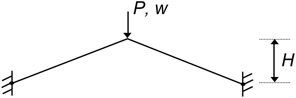
Figure 5. Schematic diagram of a toggle frame under transverse load P causing the frame to snap through with displacement w. The height H of the toggle frame is a free parameter that can be varied in a numerical continuation solver to investigate the system's snapping behavior.

The toggle frame initially deforms symmetrically on the fundamental equilibrium path. This deformation mode becomes unstable at a symmetry-breaking bifurcation just before the maximum limit point on the curve. Because the connected non-symmetric path branching from the bifurcation point is unstable, the toggle frame snaps dynamically into the inverted stable shape. In Figure 6, blue segments denote stable equilibria, red segments denote unstable equilibria and black dots denote critical points.

FIGURE 6

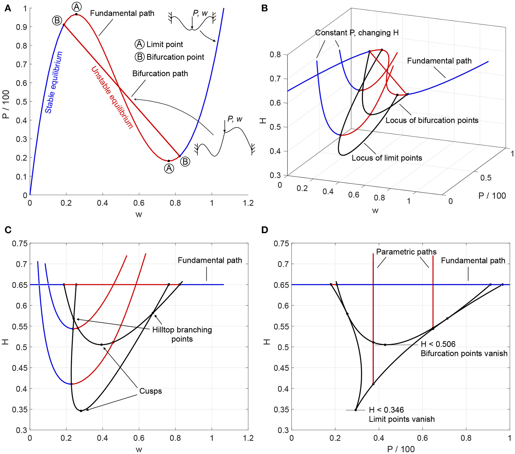
Figure 6. (A) Fundamental and bifurcation equilibrium paths of load (P) vs. central displacement (w) for a toggle frame of height H = 0.65; (B) Isometric view of fundamental and bifurcation paths in displacement-load-height space, two additional parametric paths showing the relationship between height (H) and central displacement (w) at applied loads of P = 37.4 and P = 64.8, and locus of limit and bifurcation points with changing height; (C,D) Orthographic projections of (B) in displacement-height and load-height space, respectively, indicating cusp catastrophes and hilltop-branching points.

Figure 6A restricts path-following to the classical displacement-load space. To illustrate generalized path-following capabilities, Figure 6B extends the analysis to changes in the height H of the frame. Figure 6B shows an isometric view in displacement-load-height space of the fundamental and bifurcation paths, plus two additional parametric paths. For these parametric paths, the applied load is held constant at P = 37.4 and P = 64.8, respectively, and the relationship is traced between the height H and central displacement w.

By imposing a singularity condition in the generalized path-following algorithm, the locus of limit and bifurcation points can be traced, illustrating how changes in the height of the frame affect the load-displacement solution of these singular points. There are multiple benefits of tracing such fold lines. First, they can be used to identify interesting points, such as the coincidence of limit and bifurcation points—the hilltop-branching points at H = 0.567 and H = 0.581—or points where bifurcation and limit points cease to exist—the cusp catastrophes at H = 0.506 and H = 0.346. These points are clearly marked in the orthographic projections of Figure 6C (w vs. H) and Figure 6D (P vs. H). Second, fold lines can be used in design studies to determine the sensitivity of singular points with respect to design parameters, without having to perform computationally expensive Monte Carlo studies. Finally, fold lines can be used for optimization purposes. For example, the displacement at the first instability can be maximized by reducing the height of the toggle frame to coincide with the hilltop-branching point at H = 0.567 (see Figure 6C).

3.3. Application to the Cylindrical Shell

Consider a thin-walled isotropic cylindrical shell of thickness t = 0.247 mm, radius R = 100 mm and length L = 160.9 mm loaded in uniform axial compression via displacement control. The cylinder is linear elastic and isotropic with Young's modulus E = 5.56 GPa and Poisson's ratio ν = 0.3, chosen to model Yamaki's longest cylinder (Batdorf parameter $Z=L^2\sqrt{1-{\nu }^2}/Rt=1,000$) [31]. To represent a typical experimental setup as closely as possible, the cylinder is rigidly clamped at both ends with axial compression/displacement u imposed at one end of the cylinder and the other end completely constrained.

The cylinder is modeled using isoparametric, geometrically non-linear finite elements based on a total Lagrangian formulation. The finite elements used are so-called “degenerated shell elements” [47] based on first-order shear deformation theory assumptions [48]. The cylinder is discretized into 97 axial and 241 circumferential nodes, that are assembled into 25-noded spectral finite elements using the element formulation of Payette and Reddy [49] and the large rotation parametrization described by Bathe [50]. To reduce computational effort and complexity, only a quarter of the cylinder is modeled. The circumferential domain is described by s/R ∈ [−π, π] and the axial domain by x/L ∈ [−0.5, 0.5] such that we model the quarter-segment s/R ∈ [0, π] and x/L ∈ [0, 0.5] with reflective symmetry conditions applied along the lines of symmetry. In all figures that follow, blue segments denote stable equilibria, red segments unstable equilibria, and black dots critical points.

Figure 7A shows the equilibrium path starting from a single dimple, superimposed on the pre-buckling curve (fundamental path) in terms of normalized axial compression (uR/Lt) vs. normalized load (P/P_cl). The classical buckling load is given by $P_{\text{cl}}=2\pi E{t}^2/\sqrt{3(1-{\nu }^2)}$. The stable pre-buckling curve runs diagonally in blue with the unstable single dimple solution running almost coincidentally alongside it. The unstable equilibrium branch of the latter starts at a limit point close to the first critical point on the pre-buckling path. This limit point is denoted by 0 in Figure 7A with the corresponding normalized radial (out-of-plane) displacement (w/t) shown in Figure 7B. The deformation mode clearly shows a localized dimple in the center of the domain.

FIGURE 7

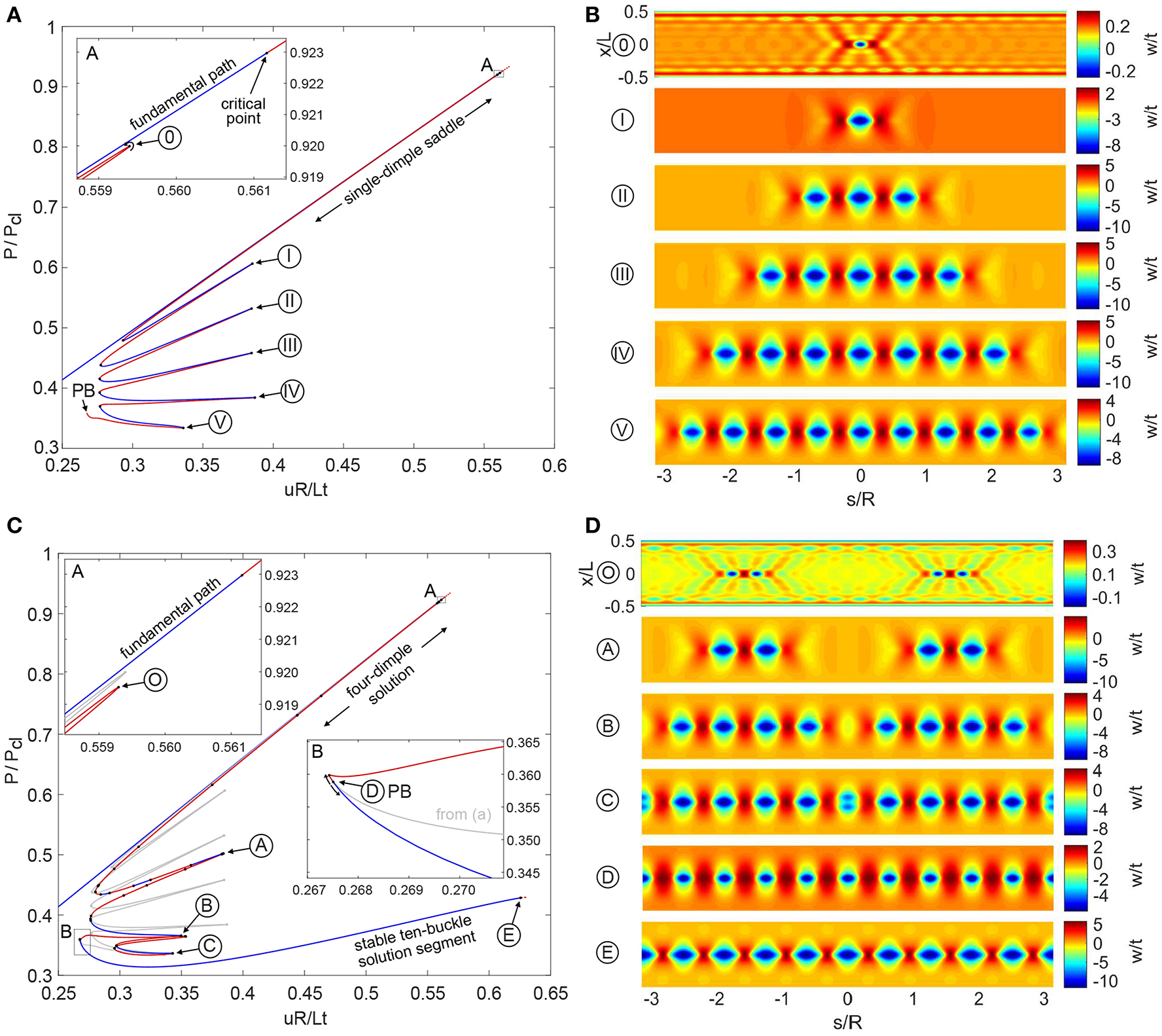
Figure 7. (A) Equilibrium path of a single-dimple post-buckling solution growing sequentially around the cylinder circumference through a series of destabilizations and restabilizations known as cellular buckling (or snaking). (B) Deformation mode shapes of the displacement component normal to the cylinder wall (w) over the cylinder domain (x is the axial coordinate and s the circumferential coordinate) for different points 0–V in (A). (C) Equilibrium path of a four-dimple post-buckling solution growing sequentially through cellular buckling. The single-dimple snaking solution in (A) connects to this path at a pitchfork bifurcation (see point D in inset B). (D) Radial deformation mode shapes over the cylinder domain for different points O–E in (C).

Path-following in the direction of decreasing displacement leads to a snaking sequence. The reason behind snaking has been established in a number of related contexts as the behavior of homoclinic orbits in the unfolding of a heteroclinic connection between flat and periodic states (see [21]) and references therein for an application to structural mechanics. The phenomenon is closely related to the notion of front pinning around a Maxwell point, first described by Pomeau [51] in the context of fluid dynamics. For a recent review of snaking see [52].

Starting from limit point 0 in Figure 7A, the single dimple becomes more pronounced with decreasing end-shortening and stabilizes at a limit point (uR/Lt = 0.293, P/P_cl = 0.479). This critical point corresponds to the smallest possible compression to allow a single dimple as an equilibrium solution. Tracing the equilibrium path further, a series of destabilizations and restabilizations add further buckles to the left and right of the original single dimple. Proceeding along the snaking path, the single dimple thus grows in a sequence of 1, 3, 5, 7, and 9 waves until an entire ring around the cylinder exists. The mode shapes corresponding to limit points I–V in Figure 7A are shown in Figure 7B and depict the series of increasing odd-numbered buckles (1, 3, 5, 7, and 9) spreading around the cylinder circumference. This snaking sequence of odd buckles connects to another equilibrium path that preserves an additional symmetry group at pitchfork bifurcation point PB. This additional path is described next.

The equilibrium path in Figure 7C is an additional snaking sequence starting from two sets of two dimples located to the left and right of the original dimple (see Figure 7D). In Figure 7C the snaking path of the single dimple (from Figure 7A) is shown in gray for reference and the new equilibrium path starting with two sets of two dimples is shown in red/blue. The four-dimple snaking path also originates at a limit point (O) close to the first critical point of the pre-buckling path (see inset A of Figure 7C). With decreasing end-shortening, the snaking sequence grows from 4 to 8, and finally to 10 buckles. The mode shapes corresponding to various points on the red/blue path of Figure 7C are shown in Figure 7D. The two equilibrium paths (gray and red/blue) are seen to connect at a pitchfork bifurcation (point D in inset B of Figure 7C). In the immediate vicinity of this connection, the four-dimple snaking path regains stability at a limit point. The ten-buckle waveform is stable from uR/Lt = 0.268 until it destabilizes at a pitchfork bifurcation (point E) at uR/Lt = 0.626. Beyond this bifurcation, an additional snaking sequence occurs, leading to the full Yoshimura post-buckling pattern. Additional rings of buckles all initiate from a single localization and then spread circumferentially (see [53] for more details).

An additional snaking sequence starting from two dimples and representing growth of an even number of waves (2, 4, 6, 8, and 10) also exists. The even snaking sequence mirrors the behavior of the odd snaking sequence in its pattern formation and in the connection to another equilibrium path at a pitchfork bifurcation. In systems featuring spatial localization, snaking of both even and odd number of localizations is typical [52] and these solutions are often intertwined. This behavior is also confirmed for the axially compressed cylinder and is shown in Figure 8.

FIGURE 8

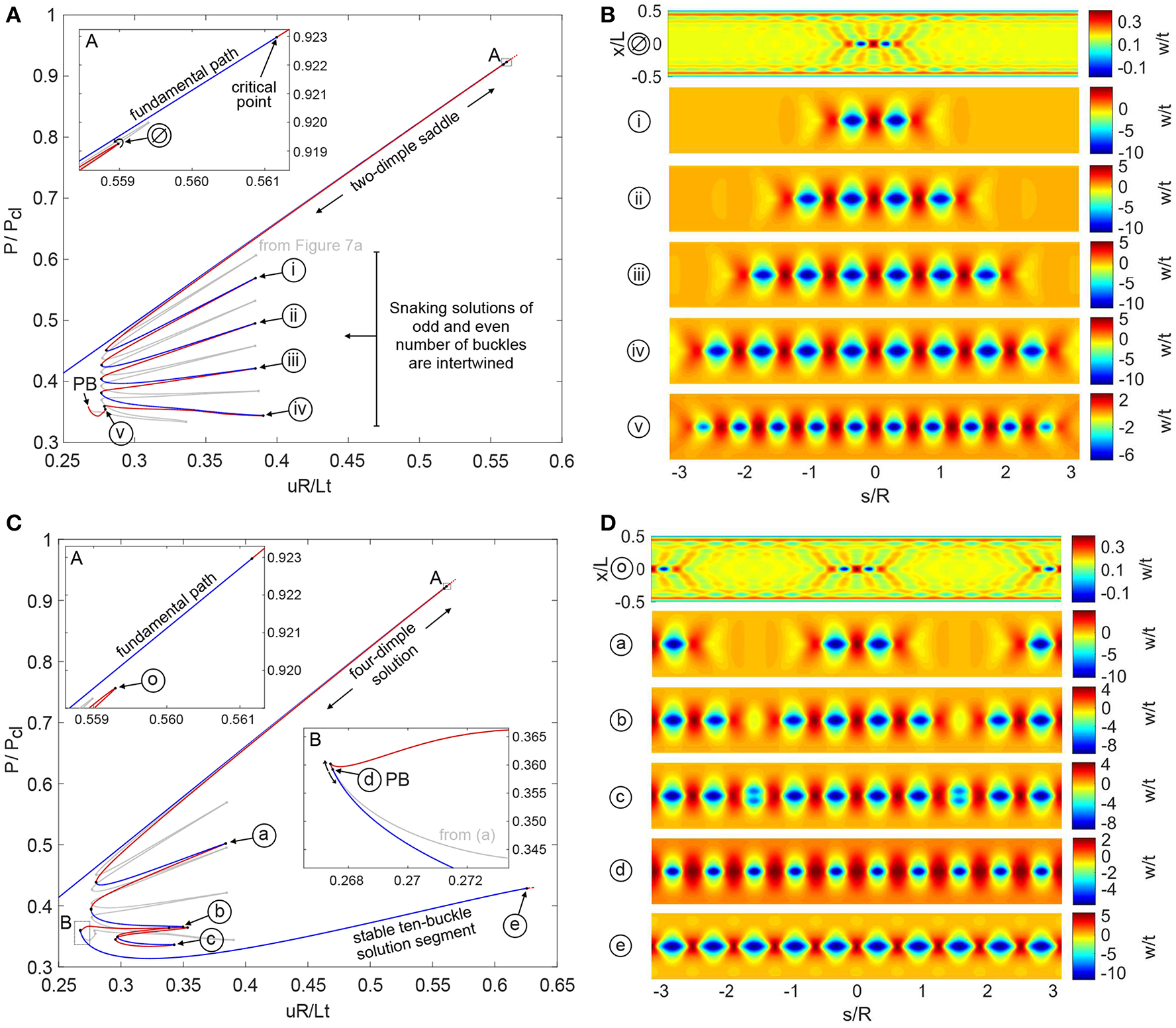
Figure 8. (A) Equilibrium path of a double-dimple post-buckling solution growing sequentially around the cylinder circumference through a series of destabilizations and restabilizations known as cellular buckling (or snaking). (B) Radial deformation mode shapes over the cylinder domain for different points ∅–v in (A). (C) Equilibrium path of a four-dimple post-buckling solution growing sequentially through cellular buckling. The single dimple snaking solution in (A) connects to this path at a pitchfork bifurcation (see point d in inset B). (D) Radial deformation mode shapes over the cylinder domain, for different points o–e in (C).

Figure 8A shows the equilibrium path of the even snaking sequence in red/blue superimposed on the snaking solution of odd buckles in gray (from Figure 7A). The even snaking sequence is also broken away from the pre-buckling equilibrium path and starts with the formation of two adjacent inward buckles (see point ∅ Figure 8B). These two buckles then multiply throughout the snaking sequence, with the equilibrium paths of the even and odd snaking sequences intertwined. The different mode shapes corresponding to limit points i–v in Figure 8A are plotted in Figure 8B and show the series of increasing even buckles (2, 4, 6, 8, and 10) growing around the cylinder circumference.

The snaking solution of even buckles also ends at a pitchfork bifurcation (point PB in Figure 8A) where it connects to another segment of the equilibrium path. This connecting equilibrium path is shown in Figure 8C with the even-buckle path from Figure 8A superimposed in gray. The two segments (red/blue and gray) of the equilibrium path connect at a pitchfork bifurcation (point d in inset B of Figure 8C). The mode shape of point d in Figure 8D confirms the expected ten-buckle waveform. In conclusion, both the odd- and even-buckle curves lead to an axially localized post-buckling state of a single ring of ten diamonds.

In closing this section we remark that the snaking results for the present paper were obtained with a mesh 4× denser than those in reference [53]. While the overall behavior of the snaking sequence and the nature of pattern formation is unchanged, the refined results presented here update and eliminate the second-order snaking features originally observed in reference [53].

4. Energy Based Methods—Maxwell and Mountain-Pass Criteria

While continuation methods are an integral part of unraveling the often complex behavior associated with subcritical instabilities, they do not tell us which state (energetically) the system would prefer, nor quantify the sensitivity of a locally metastable equilibrium state, so-called shock sensitivity. We can therefore supplement our continuation approach with energy-based methods to explore these questions more directly.

4.1. Maxwell Load vs. Maxwell Displacement

To address the problem of an infinite pre-buckling critical load (as in Figure 3B), one option is the Maxwell equal-energy criterion. This criterion originates from the concept of the Gibbs free energy in thermodynamics, to address state transitions triggered by statistical fluctuations or disturbances [54, p. 53]. Here, stability is governed only by the global minimum of total potential energy. Under some form of parametric variation, such as load or applied displacement, the Maxwell criterion provides the first circumstance for which the energy of a post-buckled state first falls below the energy minimum of the pre-buckled state. The reasoning is that, upon increase of the parameter, this would be the first time the system could be shaken out of its trivial state and transition to the post-buckled global minimum. Although the Maxwell criterion cannot be considered a hard and formal point of instability, it may, nevertheless, serve as a useful and robust lower-bound estimate for instability in systems where small disturbances and imperfections have pronounced effects.

A long structural system loaded axially typically prefers a localized to a distributed post-buckled response [32]. If the localized buckle subsequently restabilizes, additional cells of buckling will often develop in adjacent positions to the first via a sequence of localized instabilities, according to the snaking mechanism described for the cylinder above. Typically, the load tends to fluctuate or snake between upper and lower limits as the sequence progresses. The Maxwell load, defined (as above) as the lowest load for which the post-buckled energy matches its pre-buckled counterpart, lies between the two limits, and effectively acts as an organizing center about which the post-buckled load oscillates as the snaking progresses.

This snaking sequence with localizations developing over the length of a structure has now been recognized in a number of different circumstances (see for example [55–59]). However, in section 3.3 we describe an alternative snaking scenario, in which localized buckles trigger not axially but orthogonal to the direction of the applied load, around the circumference of a buckling cylindrical shell. In this sequence, a Maxwell displacement rather than a Maxwell load acts as the organizing center, with the system fluctuating between two limits of end-shortening as the load continues to fall. Two examples of such snaking behavior are seen in Figures 7A,C.

4.2. Mountain Pass Algorithms

First introduced by Ambrosetti and Rabinowitz [60], the Mountain Pass Lemma is a fundamental mathematical tool for proving the existence of stationary points of non-linear functionals. Excluding some technical details, the key ingredients of the theorem are:

1. a suitable (energy) functional ${W}(x)$

2. a stationary point e₁, which is a local minimum

3. a second point e₂, for which ${W}(e_1)>{W}(e_2)$

We note that a suitable function is normally available in the form of total potential energy, with local minima appearing on a stable fundamental equilibrium path [7].

The theorem states that, over the set of all continuous paths connecting e₁ and e₂, i.e.,

$\begin{array}{l}\Gamma :=\left\{\gamma \in C\left[0,1\right]:\gamma (0)=e_1\text{and }\gamma (1)=e_2\right\},\end{array}$

one can find the infimum of the maxima of the energy functional ${W}(u)$ along any path γ ∈ Γ. This infimum is the mountain pass solution and is a saddle point

$x_c:=\underset{\gamma \in \Gamma }{\inf }\left[\underset{x\in \gamma }{\max }{W}(x)\right].$

The physical significance of the mountain pass is that it represents the connecting point in solution space with the smallest energy hump,

$\Delta {{W}}_c={W}(x_c)-{W}(e_1),$

required to escape the local minimum at e₁ and transition to a lower energy state at e₂. Therefore, the Maxwell load/displacement (depending on the loading regime), at which ${W}(e_1)={W}(e_2)$, marks the onset of the ability to jump to such a lower energy state, and therefore the onset of “shock sensitivity” in the system.

The application of the Theorem provides a computable energy hump to assess shock sensitivity; the mountain pass state x_c itself is significant, since at this point the system has just one negative eigenvalue for which the system is unstable. This eigenvector marks a direction in solution space m tangent to the mountain path γ, and suggests a mode shape that if applied to the system would most easily induce transition from e₁ to e₂. This eigenvalue at the mountain pass point therefore indicates the imperfection or probing modes that a subcritical system could be most sensitive to.

The literature gives a variety of algorithms for finding mountain pass solutions e.g., the nudged elastic band method [61], the dimer method [62], and conjugate peak refinement [63]. Here we briefly describe the latter, as it is used later to illustrate shock sensitivity of the axially-compressed cylinder.

Conjugate peak refinement is an iterative scheme performing alternating line search maximization and minimization steps to find the mountain pass solution x_c. The approach generates a sequence of piecewise-linear approximations to a path γ^⋆ which passes through x_c. For the k^th iteration, we denote this approximation γ^(k) characterized by a set of points ${\Gamma }^{(k)}:={\left\{{\text{x}}_i^{(k)}\right\}}_{i=1}^{k+1}$. We start the process by defining γ⁽⁰⁾ as the straight line connecting e₁ and e₂, so that ${\Gamma }^{(0)}=\left\{e_1,e_2\right\}$. Then starting with k = 1, each iteration comprises three steps:

1. Line Search Maximization: We maximize the functional ${W}(\text{x})$ along the piecewise linear path γ^(k−1), to obtain line maximization point ${\widehat{\text{x}}}^{(k)}$ lying between points ${\text{x}}_j^{(k-1)}$ and ${\text{x}}_{j+1}^{(k-1)}$.

2. Line Search Minimization: We then find the scalar α such that ${W}({\widehat{\text{x}}}^{(k)}+\alpha s)$ attains a minimum, where the search direction s is chosen to be:

$\begin{array}{cc}s=-g+\frac{g^{T}h}{d^{T}h}{d}^T\text{where}d=\nabla \left({\gamma }^{(k)}\right)\text{and}g=\nabla {W}({\widehat{x}}^{(k)})& (12)\end{array}$

3. Update Mountain Path γ^(k): We then add the new point ${\widehat{\text{x}}}^{(k)}+\alpha s$ to the path to form γ^(k), so that points defining the line are

${\Gamma }^{(k)}:={\left\{x_0^{(k-1)},\dots ,x_j^{(k-1)},{\widehat{x}}^{(k)}+\alpha s,x_{j+1}^{(k-1)},\dots ,x_k^{(k-1)}\right\}}_{i=1}^{k+1}.$

At any iteration of the state ${\widehat{\text{x}}}^{(k)}+\alpha s$ is the best approximation of the mountain pass solution. Convergence can be tested by ensuring (1) the gradient of the energy at this point zero (2) determining the lowest two eigenvalues of the energy's Hessian, since only the smallest must be negative.

We now demonstrate the mountain pass procedure geometrically with a generic, two degree-of-freedom energy landscape given by a modified Müller-Brown potential [64]. This particular potential (Figure 9) has application in computational chemistry [63]. It is chosen since it has no symmetry, and is characterized by two local minima at e₁ and e₂, with a non-trivial mountain pass connecting them. The approach provides a good approximation to the saddle point in just two iterations. In the first iteration, we see the algorithm starts by approximating the mountain path with a straight line between the e₁ and e₂. A maximum is located along this line; see the ° in the far left panel of Figure 9. A minimum in the conjugate direction (12) is then found, as indicated by the symbol Δ in the next left-most panel. Thus, the first iteration provides a reasonable approximation to the saddle. The path γ⁽⁰⁾ is updated to γ⁽¹⁾, characterized by three points connected by the pair of straight lines. For iteration 2 the procedure continues in the same way, first a maximization step over the path to produce the second ° in the third panel of Figure 9, followed by a minimization problem in the conjugate direction to the path through the maximum point. For this example, the newly found minimum on this path (the second Δ in the right-most panel of the figure) satisfies the tolerance condition

$\begin{array}{l}\left|\right|\nabla {W}({\text{x}}_c)|{|}_e<ϵ=1\times 10^{-5},\end{array}$

and the algorithm terminates.

FIGURE 9

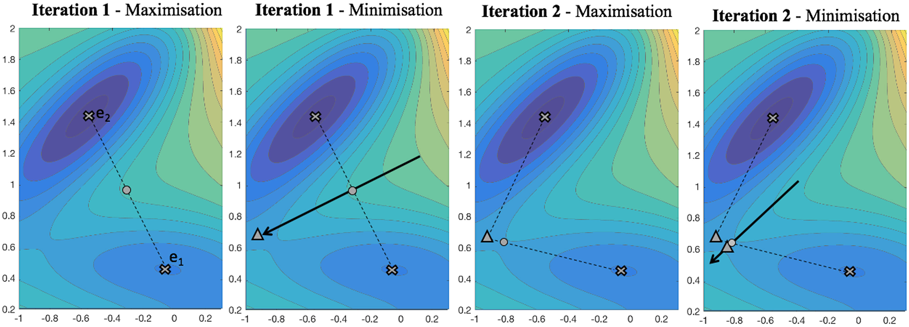
Figure 9. Symbols denote: (×) Local minima, (−−−) potential “mountain path,” (→) search direction ○ line maximum, Δ line minimum.

4.3. Application to the Cylindrical Shell

Classically, stability of equilibrium is governed entirely by the local Hessian of the total potential energy; wells with respect to all degrees-of-freedom denote stability, whereas saddles or maxima denotes instability. This framework fails in the case of infinite critical loads presented in Figure 3, where two equilibrium paths are separated by a small energy barrier but never strictly intersect. Thus, although the idealized structure never transitions out of the trivial equilibrium state, that state becomes metastable, where small disturbances could trigger instability.

As is seen in the insert of Figure 7A, the cylinder too features an equilibrium path that asymptotically converges to, but never actually intersects, the pre-buckled path. Here, we compare the energy levels of the pre-buckling path and the circumferentially periodic equilibrium path of a single ring of diamonds (path ending in point E in Figure 7D). As load is applied in a rigid manner (controlled end-shortening), the stability threshold corresponds to a Maxwell displacement and this computes to be M_u = u_M/u_cl = 0.486 (u_MR/Lt = 0.294). It is interesting to note that this value correlates well with the limit point (uR/Lt = 0.294) in Figure 7A.

The Maxwell displacement could serve as a lower-bound estimate for the cylinder's first instability load, by marking the onset of “shock sensitivity” [65]—i.e., that of metastability of the pre-buckling path. This snaking sequence marking the development of a single dimple into a buckle pattern that is periodic circumferentially but localized axially, is in marked contrast to the snaking at the lower Maxwell load of such rings developing to a fully periodic pattern identified in earlier work [40, 66].

Rather than apply a computationally expensive infinite degree-of-freedom mountain-pass algorithm as in Horák et al. [35], another way of looking for the mountain-pass solution is to test the cylinder's resilience to the single-dimple localization; how much displacement is necessary to trigger a dynamic escape from stable pre-buckling to a post-buckled state via the mountain-pass saddle? We could envisage perturbing the cylinder from the side using a hypothetical infinitesimally-thin, infinitely-stiff, probe or poker; experimental implementation of this idea is explored in section 5 below.

To implement such an analysis numerically, consider applying such a poker at right angles to the cylinder mid-surface, half-way along its length. Such a process involves two fundamental parameters, applied end-compression u and lateral probing force F. We consider applying such a probe repeatedly as the axial compression is quasi-statically increased. The results are presented in Figure 10. At low levels of axial compression, we find a non-linear softening/stiffening relationship of strictly positive stiffness between the probe force F and the ensuing dimple displacement Δw; see path 1 in Figure 10A. Here Δw denotes radial displacement relative to the radial (Poisson) dilation that naturally occurs in the pre-buckling state.

FIGURE 10

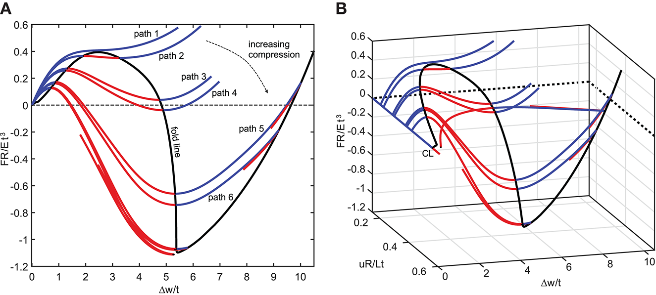
Figure 10. The stability landscape of an axially compressed cylinder with a probing side force. (A) Normalized probe force (FR/Et³) vs. normalized probe displacement (Δw/t) for different values of normalized axial compression (uR/Lt). (B) The stability landscape in terms of axial compression vs. probe force vs. probe displacement.

For increased levels of end-shortening, the equilibrium manifold traces S-shaped curves; as the dimple develops, lateral resistance reduces, until limit points are traversed leading to regions of negative stiffness (paths 2–3 in Figure 10A). For even greater end-shortening, the probe force reduces significantly, dipping below the zero load axis (e.g., F = 0 on path 4). At this point an unstable saddle state is encountered, corresponding to the single-dimple mountain-pass solution. Also shown in Figure 10A is a black fold line connecting maximum and minimum limit points, and thereby describing a boundary that separates the domain into stable and unstable regions.

Figure 10B expands this landscape into three dimensions, providing an interesting stability landscape that qualitatively matches the experimental results of Virot et al. [67] on a different cylinder. The area between the stable pre-buckled and unstable single-dimple solutions under the F vs. Δw curve represents the energy barrier, and thereby the “shock sensitivity” of the pre-buckling state. The size of this energy barrier can be understood qualitatively by plotting the fold line connecting maximum and minimum points; see Figure 10B. This curve slopes down toward the buckling point on the pre-buckling path (point CL). Indeed, the fold line intersects the buckling point on the pre-buckling path, confirming that resilience of the pre-buckling state to small perturbations (i.e., the linear stability) indeed vanishes at that point.

5. Experimental Methods for Exploring Instabilities

While numerical methods for the analysis of non-linear structures are well-developed, experimental methods tailored to such structures, in particular shell buckling, have received comparatively little attention (see e.g., [20, 31, 67–72]). The trend in modern engineering is to test experimentally for single parameter values, and then use computational models, virtual testing, and “digital twins” wherever possible to extend the envelope. However, for fundamentally imperfection-sensitive buckling problems, such an approach will not explore the stability landscape reliably. Hence there is a fundamental barrier to researchers hoping to exploit non-linear structures concepts for industrial applications. This barrier has arguably led to over-conservative designs in safety-critical industries like the aerospace sector, which requires stringent testing before new components are allowed to fly. Organizations, such as NASA have therefore put renewed emphasis on experimental testing, and in particular, feeding high-fidelity imperfection measurements of specimens into models [72].

5.1. Experimental Path-Following

Conventional test methods fail to capture all but the simplest non-linear behavior, and consequently researchers lack reliable methods to validate their ideas experimentally. The main reason traditional test methods fail is the difficulty in measuring unstable parts of the response. Any structure whose equilibrium curve features limit points can snap under force- or displacement-controlled test methods, as illustrated in Figure 11A. Such snap-through thus gives rise to regions of the equilibrium curve that might seem inaccessible experimentally.

FIGURE 11

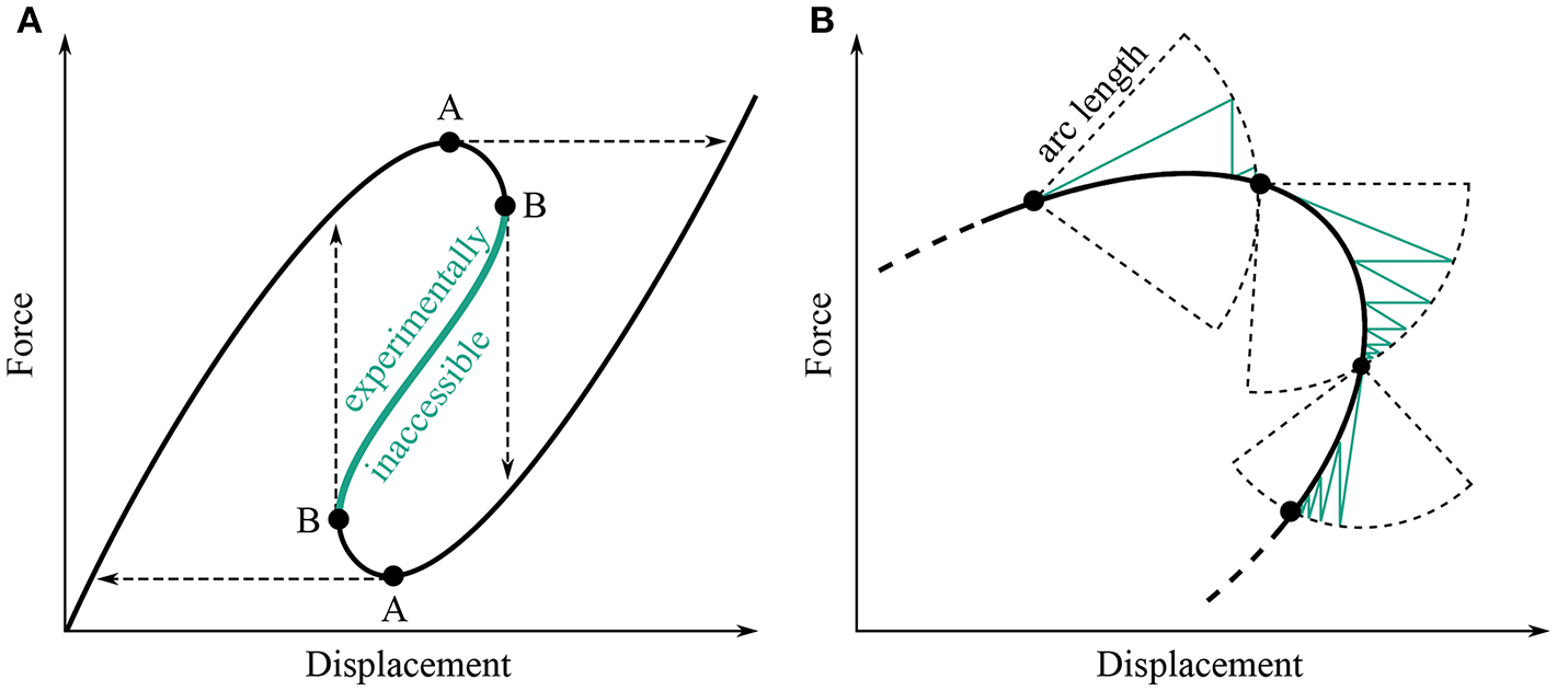
Figure 11. (A) Schematic of a non-linear force-displacement curve featuring both displacement and force limit points. At a force limit point (A) force-controlled test methods snap across. At a displacement limit point (B) displacement-controlled methods snap down. (B) Schematic of an arc length-based numerical solution traversing a displacement limit point. The green line represents the iterative solutions of a Newton-Raphson based method.

Numerical analysis succeeds where experiments fail because in a numerical setting the force and displacement at a control point can be controlled independently and simultaneously. This freedom allows the solver to set combined limits on force and displacement, and prevents jumping to other solutions when an equilibrium becomes unstable (see Figure 11B for an illustration of the arc-length method). Consequently, displacement limit points can be traversed, unstable paths followed, and the full non-linear response of a structure described. In an experimental setting, the force and displacement of a control point are linked by the elasticity of the structure; meaning that one can control the displacement of a control point and generate a reaction force, or vice versa, but not both. This coupling makes it impossible to apply numerical techniques to experiments without some additional control.

There are several interesting published approaches to work around this problem. Wiebe and Virgin [73] use a hammer to trigger snap-through of a shallow arch. By analyzing the transient dynamic trajectories of the structure during the snap, locations of unstable static equilibria are deduced. By intentionally allowing snap-through, this method can locate unstable equilibria without needing to actively control them. Virot et al. [67] use a poker to laterally probe a cylinder under increasing axial load. By tracking changes in the probe force-displacement curves, they can estimate the load at which the cylinder becomes globally unstable, before the instability load is reached. The concept of probing is especially relevant to the work presented here: an experimental path-following method which utilizes probes to stabilize and control unstable equilibria.

5.2. Application to a Shallow Arch

Consider the centrally-loaded shallow arch studied by Neville et al. [74] shown in Figure 12A, with dimensions L = 205 mm, h = 20 mm, t = 1.5 mm, and depth = 5 mm. For symmetric deformations, the structure exhibits the complex non-linear behavior shown in Figure 12C. Looking at the first few “petals” (starting at one of the two fundamental equilibria and following the equilibrium path toward the other), it is clear that the response comprises many successive displacement limit points. A displacement-controlled experiment would only obtain the first two segments of the equilibrium curve (the solid lines in Figure 12D), snapping from one to the other at limit points L₁ and L₂.

FIGURE 12

Figure 12. (A) Geometry of the shallow arch. The depth of the arch is not labeled; this dimension is measured into the page. Displacement u_a is applied at the mid-span actuation point, generating reaction force F_a. (B) Modified geometry including two “probes.” Symmetry is maintained by enforcing vertical displacement u_p across both probes, while they are allowed to move horizontally. (C) FEA prediction of the full equilibrium curve from one fundamental state to the other. (D) A subset of the equilibrium curve, starting from each of the fundamental equilibria and showing only the first two limit points on each side; equilibria available at u_a = 5 mm are numbered 1–5. (E) Deformation shapes associated with equilibria 1–5. This figure has been redrawn from the figures in Neville et al. [74].

At u_a = 5 there are several equilibria available; each with distinct values of F_a. Each equilibrium is also associated with a unique deformation shape (Figure 12E), where the unstable equilibria correspond to more complex shapes. Controlling the structural shape allows us to stabilize unstable equilibria, and indirectly influence the reaction force on a displacement-controlled control point. Having decoupled the force and displacement experimentally, numerical approaches become viable. Two extra probes provide control over the deformation shape as shown in Figure 12B. Such probes produce reaction forces that change the structure. However, when the probe reaction force equals zero, then it is an equilibrium of the unperturbed structure. Crucially, reaction force is also zero at unstable equilibria—in this case the probes provide the infinitesimal restoring force required to prevent the instability from growing. By applying a large probe perturbation at a stable equilibrium, the probes can be used to search for other equilibria.

By moving the probes and actuation point in concert, a simple form of path-following can be performed [75]. The actuation point steps forward, then the probes search for equilibrium (F_p = 0). Small perturbations can be used to avoid large deviations from the equilibrium curve. If the actuation point steps past a limit point, the probes will not be able to find equilibrium and the actuation point direction is then reversed. This approach allows the equilibrium path of the shallow arch to be followed around a displacement limit point, as shown in Figure 13B. The FEA prediction is also shown in Figure 13A, for comparison. Deformation shapes of the arch at several points in the experiment are also shown in Figure 13C. Shapes 1 and 2 are the two fundamental equilibria (also shown in Figure 12C). Shape 3 corresponds to a stable equilibrium, and resembles shape 1 in Figure 12E. Shape 4 corresponds to an unstable equilibrium, and consequently is more complex. It resembles shape 2 in Figure 12E, which corresponds to the same segment of the equilibrium curve.

FIGURE 13

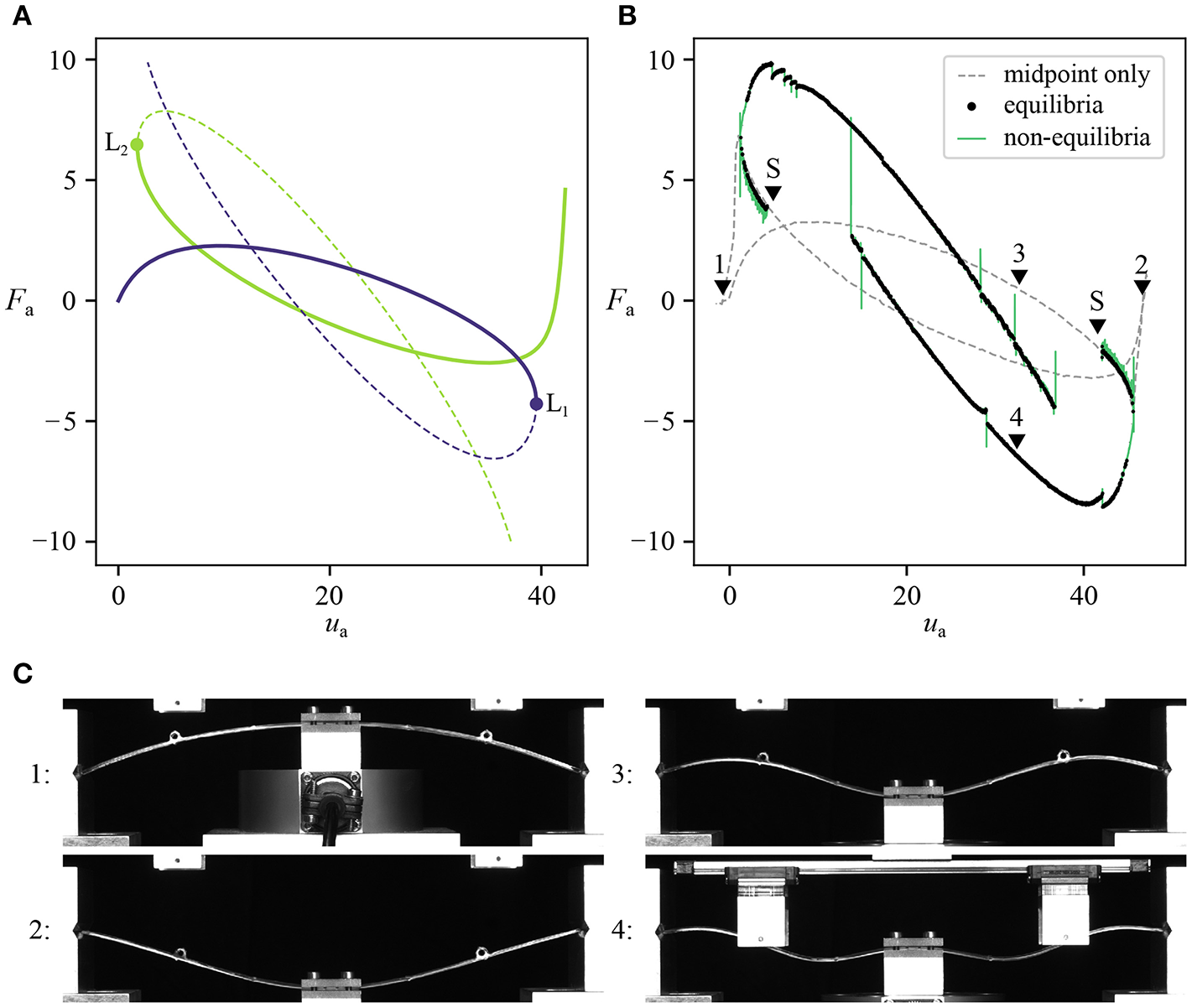
Figure 13. Results of the experimental path-following method. (A) FEA prediction of a subset of the equilibrium curve. Solid and dashed lines indicate stable and unstable segments, respectively. (B) Equilibrium curves obtained in a path-following experiment from Neville et al. [76]. The dashed gray line was obtained using displacement control on the midpoint only. The path-following algorithm was started at the two points marked “S.” Non-equilibria (e.g., |F_p| > 0.1 N when searching for equilibria) are shown in green, and equilibria (F_p < 0.1 N) are indicated by the black dots. (C) Deformation shapes of the arch during the experiment. Shapes 1–4 correspond to the markers 1–4 in (B).

Experimental results are naturally affected by phenomena and imperfections not included in theoretical models. The shallow arch example, for instance, is sensitive to changes in geometry and probe location, as well as displaying complex behavior in response to the two input parameters (u_a and u_p). Virtual testing is a technique that can address these issues, and aid in experimental design and interpretation of results. A successful example of such a virtual testing environment coupled to the commercial FE solver ABAQUS is presented in Groh et al. [75]. A finite-element model is used to simulate a “perfect” experiment—i.e., one in which the equipment and test specimen behave exactly as intended. The model includes limitations of the experimental setup—e.g., sensor noise, limited number of control points, etc.—and provides the same inputs and outputs that are available in the real experiment. This virtual testing environment provides a useful middle ground between numerical solutions and experiments, and serves as a “sandbox” or digital twin to explore the effects of different test configurations and imperfections.

5.3. Experimental Mountain-Pass Methods—“A Game of Poker”

Inspired by the theoretical work of Horák et al. [35], Thompson et al. [11, 65] observed that the mountain-pass state for an axially-compressed cylinder looks remarkably similar to the small dimple induced by probing the cylinder laterally with a finger. The authors discuss a thought experiment where the cylinder's resilience to perturbations (i.e., linear stability) is tested by probing the cylinder radially inwards using a poker (see Figure 14).

FIGURE 14

Figure 14. Test for assessing the resilience of the cylinder to perturbations, proposed by Thompson [65] and Thompson and Sieber [11].

In fact, the idea of poking axially-compressed cylinders from the side to assess resilience to buckling has a long history predating any mountain-pass considerations. By tapping axially-loaded cylinders with a finger, Eßlinger and Geier [77] found stabilized single-dimple states. Hühne et al. [71] realized that the single dimple can act as an imperfection, that excites the characteristic observed buckling behavior. They set out to out to determine a robust lower bound to buckling load that could replace the empirically determined knockdown factors proposed in NASA's SP-8007 [78] guideline. Over the last decade, this methodology has led to a battery of tests on composite cylinders [79], and extensions to probabilistic perturbation [80] and multiple perturbation loads [81].

The poker force vs. displacement response of the cylinder for different levels of axial compression was shown previously using FE simulations in Figure 10A. Once these S-shaped curves pass through the zero-poker-force axis, the single dimple exists as an unstable saddle solution and a dynamic escape via the mountain pass is possible. The likelihood of such an escape can be quantified by the mountain-pass energy barrier, represented by the area enclosed by the associated force/displacement curve and force axis. In Figure 10A it is readily observed that the greater the applied axial compression, the smaller the energy barrier provided by the single-dimple mountain pass. Thus, by repeating the poking procedure for multiple levels of axial compression and computing the energy barrier up to the mountain-pass point, a non-destructive testing method can be established that provides a safety cushion before buckling is likely to occur.

Such a probing experiment was successfully implemented by Virot et al. [67]. By controlling the displacement of the lateral poker, the unstable mountain-pass point was determined when the reaction force on the poker vanished; this state replicating that of an unprobed cylinder. Furthermore, by aggregating the poker force vs. poker displacement curves for multiple levels of compression, a stability landscape emerged that qualitatively matched (Figure 10B). An experimental buckling load of the cylinder could also be determined by recording the level of compression for which it lost its ability to resist the poking displacement, i.e., the reaction force fell beneath a specific tolerance.

Even though the idea is simple to implement, in practice the system can bifurcate by pivoting around the point load. To offset this symmetry-breaking effect, as highlighted by Thompson and Sieber [11], a second control probe is often required. Second, the choice of probing location needs to be carefully chosen, as different locations can lead to differing buckling load predictions [82]. Finally, there are practical shortcomings to obtaining the mountain-pass state for arbitrary systems. For the cylinder, the mountain-pass state happens to be a relatively simple single-dimple localization, but in general, it could be more intricate, and may be difficult to impose by one or even multiple pokers. Combining poking experiments with experimental path-following algorithms may well prove a fruitful avenue for future research.

6. Exploiting Buckling Instabilities

As stated in the Introduction and indeed reflected in the title of this paper, instability need not solely be considered as something to be avoided or designed against; it is also possible to utilize instability in a positive manner [3]. We highlight three areas where such benefits can be found in different engineering domains and length-scales.

6.1. Prestressed Stayed Columns

Prestressed stayed columns are important elements of many modern large-scale structures; see Figure 15.

FIGURE 15

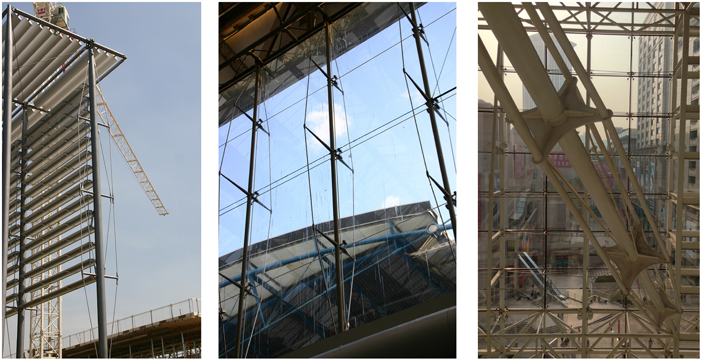
Figure 15. Prestressed stayed columns in practice. (Left to right) An example as a slender support for a façade in Chiswick Park, West London; a set of roof supports in the former Eurostar terminal in Waterloo Station in Central London; an example in a shopping mall in Dalian, China. Photographs courtesy of Dr. Daisuke Saito and Dr. Jialiang Yu.

Such columns tend to be slender and have intermediately placed cross-arms and associated pretensioned cables, thereby reducing the buckling effective length L_e. The length L_e provides a measure of the critical buckling eigenmode wavelength and the Euler strut buckling load is proportional to $1/L_e^2$. The system of cable stays and cross-arms in the prestressed stayed columns provide intermediate restraints that reduce L_e significantly and hence provide a commensurate increase in critical buckling load and ultimate capacity. Depending on the overall geometry, this change in critical buckling load can also be associated with quantitative and qualitative changes in the triggered buckling mode within the non-linear range. The behavior has been discussed at length in previous work, with the focus falling on qualitative critical [83] and post-buckling behavior determined by the pretensioning force [84], physical experiments [85], triggering of modal interactions and associated symmetry-breaking [59, 86] and tuning behavior for different cases [87, 88].

Some of these works use conventional finite element modeling, where post-buckling shapes are initiated by introducing imperfections that are affine to linear buckling modes. A drawback is that the full picture of modal interaction only becomes available under a combination of symmetric and anti-symmetric imperfections. Other modes may also be drawn in, for example, should it be thin enough, localized buckling in the main tubular column, and the numerical methodology discussed in section 3.3, can be useful. Nevertheless, there has been a sequence of increasingly-sophisticated low-dimensional models, to capture mode interaction [59, 89]. These models are based on the Rayleigh–Ritz method, with a finite number of linear eigenmodes of the unstayed column being used to discretize the deformation response, with cross-arms acting as beams, and cable stays as tension-only members.

The particular complication in stayed columns is produced by the cable stay, where there is the possibility of a sudden loss in elastic stiffness caused by cables slackening. The outcome is similar to that described in Figures 2D, 3C. Using numerical continuation it has been possible to track post-buckling paths of perfect systems within the package AUTO-07P [45]. Figure 16 shows a realistically-proportioned symmetric stayed column system of length L with three cross-arms of lengths a_e and a_m, the exact details of which are presented in Yu and Wadee [59]. It shows that the mechanical response is likely to destabilize when distinct modes are triggered or mode interaction dominates; the kinks in the post-buckling paths are signatures of the portions of the cable stays going slack, instantly losing axial stiffness, and causing a sudden unstable jump in the response.

FIGURE 16

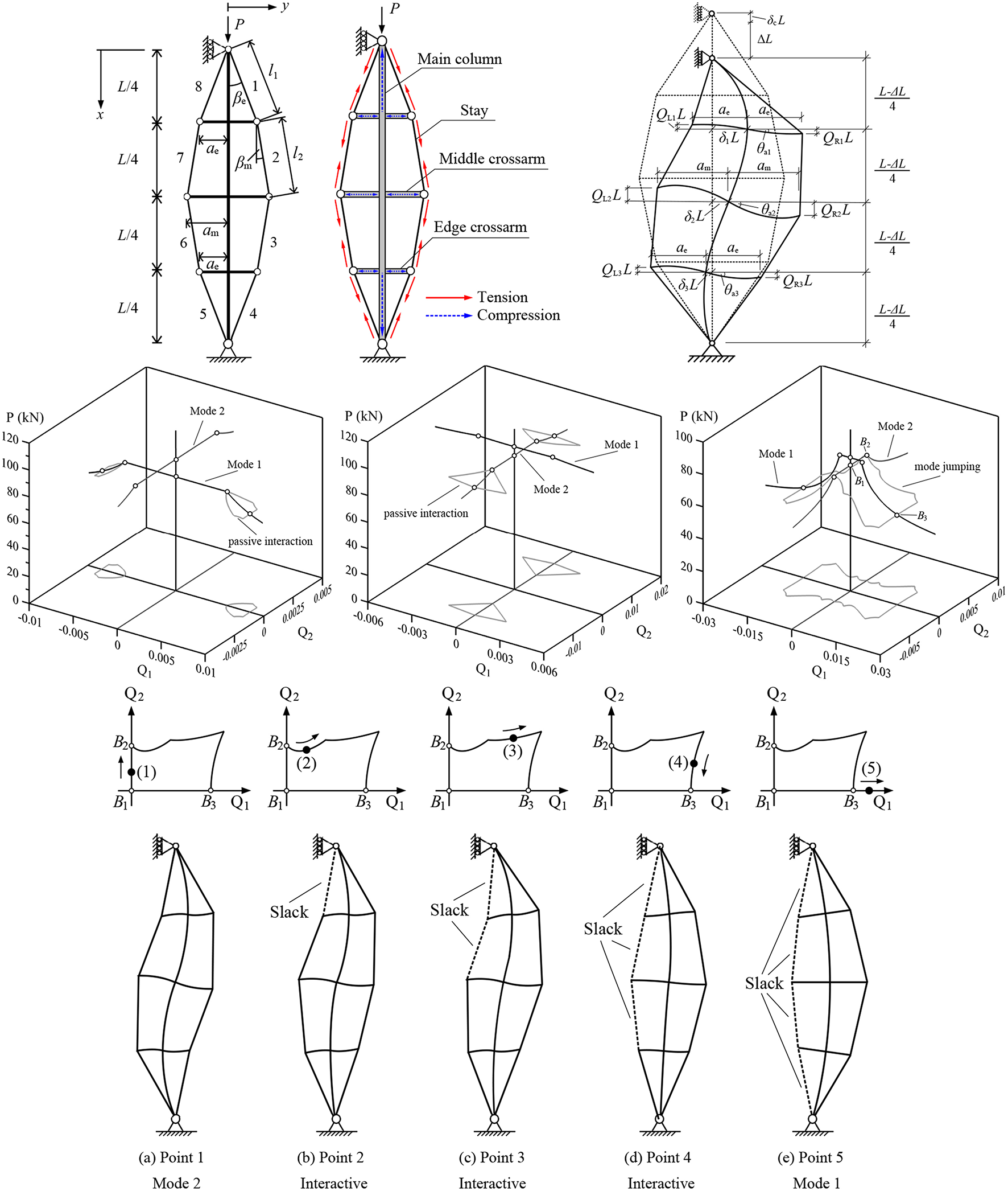
Figure 16. Prestressed stayed column. (Row 1: left to right) Geometric definitions; effect of prestressing and buckled shape showing deformations of main column, cross-arms and stays used in the Rayleigh–Ritz model. (Row 2: left to right) Equilibrium paths showing: distinct mode 1 buckling (Q₁); distinct mode 2 buckling (Q₂); interactive buckling with a secondary mode jumping path. (Rows 3–4) Illustration of mode jumping through different points on the secondary mode jumping path from the third case in row 2 now plotted as Q₁ vs. Q₂ in row 3 and the deformed structure presented in row 4.

The column subsequently restabilizes once it finds a configuration that restores equilibrium. Both the numerical continuation procedure for the analytical model, and the Riks algorithm used in ABAQUS, can capture this behavior. One advantage of the former is that it tends to crystallize the detailed mechanical response into a few distinctive characteristics; the main column buckling modes are discretized into a Rayleigh–Ritz type model, and the non-linear results provide straightforward output of the contributions of the linear buckling modes to the post-buckling profile, Q₁ and Q₂ being amplitudes of the first two main column buckling modes. This analysis allows the interpretation of the effects of symmetry-breaking, and the potential to trigger higher pure or interactive modes in the post-buckling range.

All the consequences for the post-critical strength, stiffness and potential to jump between different equilibrium states owing to the cable stay behavior, can be determined directly. This information can then be used to determine parametric spaces where practical geometric quantities, such as stay diameter, layout of the stayed column system and initial prestressing forces, can generate qualitatively different, yet predictable, responses [59, 87], as shown in Figure 16.

The simplest configuration with a single-cross arm can also be considered as a single cell within a larger lattice material. The performance of metal lattices, for example with a criss-cross structure as in Queheillalt and Wadley [90], may be enhanced by including internally woven tension ties, to make them similar to woven composites [91]. The behavior of the sandwich panel of Figure 17, depends on non-linear interactions between the individual cells, and is observed to have a similar structure to the stayed column. By adjusting the pretension in the ties at the production stage, alongside the geometry of the cells and the overall configuration, it is possible to engineer the post-buckling stiffness to a desired level. If, for instance, the post-buckling stiffness of an overall panel can be tuned to be practically zero [92], but with each buckling cell having a significant critical load, then the structure would be highly effective in absorbing energy. Moreover, since stress propagation depends on structural stiffness, if the post-buckling stiffness on the panel were zero, it would potentially minimize stress transfer to any attached structure. This type of application, using internal buckling of a lattice material for dynamic isolation purposes, has potential for applications where lightweight reusable elements are required for impact and blast protection or seismic isolation [93].

FIGURE 17

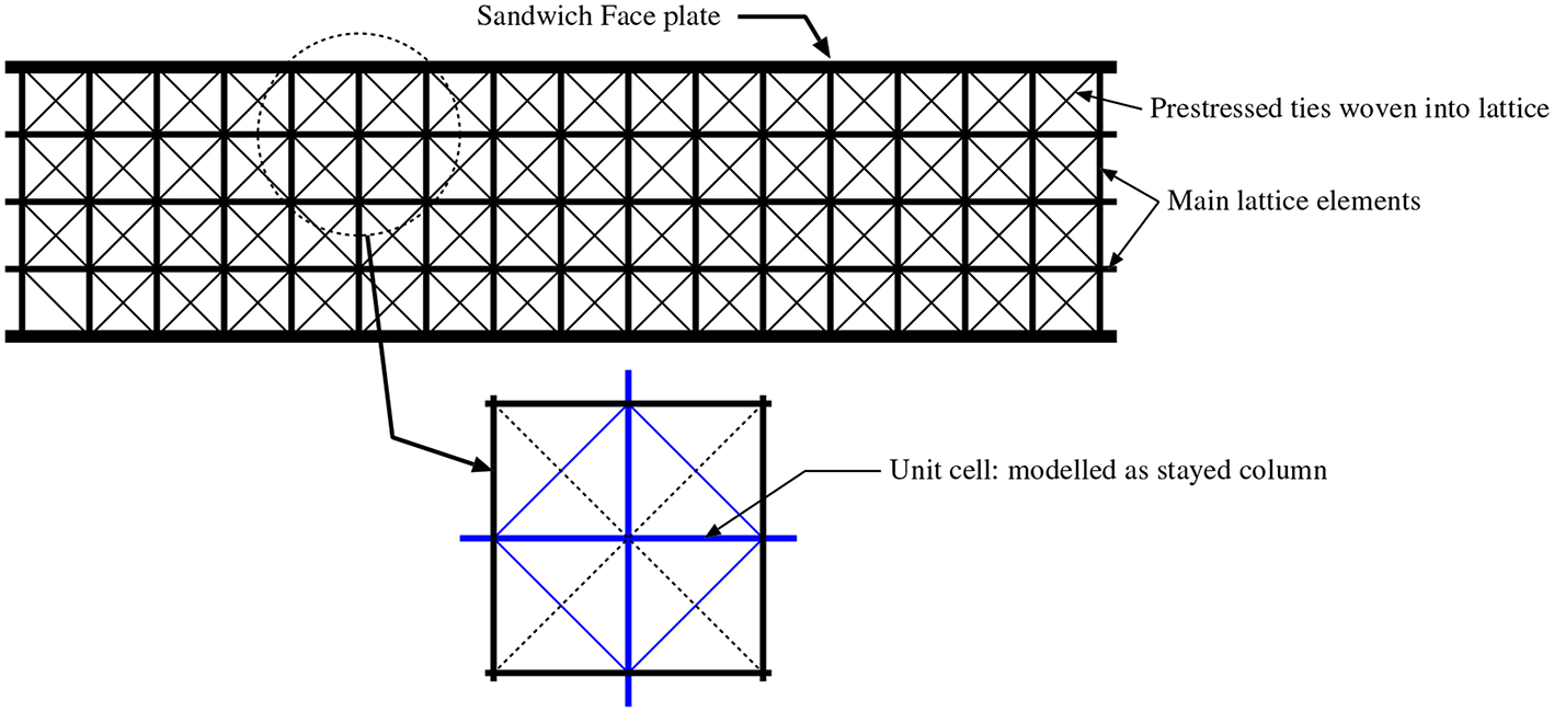
Figure 17. Sandwich panel with prestressed lattice core, the unit cells of which can be represented as prestressed stayed columns, as highlighted in the lower diagram [90, 91].

6.2. Adaptive Structures

So-called adaptive structures are able to change shape and/or material properties in response to varying external stimuli [94]. The application of adaptivity in engineering has the potential for significant improvements in performance, by making structures more efficient over a broad range of operating conditions [95]. A fascinating natural example of shape-adaptivity is the Venus flytrap, whose rapid transition from open to closed to capture its prey occurs as a consequence of snap-buckling instability [96]. Hence, when operating conditions require large displacements and/or multiple stable configurations, structural instabilities can be viewed as potentially advantageous rather than a source of failure.

Consider for simplicity the buckling response of a simply-supported Euler strut, illustrated in Figure 18. In particular, consider the stable post-buckled configuration in the inset of Figure 19A. For given combinations of compression and symmetry-breaking defects, such a post-buckled structure can behave like an arch, exhibiting dynamic “snap-through” behavior between the two stable states when subjected to an external transverse load, F. For a beam compressed just beyond the first buckling load, these configurations connect via an S-shaped equilibrium path in the space of a centrally-applied force, F plotted against the midpoint respective deflection δ, as shown graphically in Figure 19A. The structure initially deflects in a stable manner before reaching a maximum limit point, where it snaps dynamically through a region of instability (2) onto the equilibrium branch for its second stable configuration (3).

FIGURE 18

Figure 18. Buckling of a simply-supported strut and corresponding equilibrium diagrams. (A) The strut deflects sideways when subjected to a compressive force greater than the buckling load. (B) An idealized symmetric strut with no geometric or loading imperfections features a symmetric pitchfork bifurcation diagram in load vs. displacement space. (C) Initial imperfections break the pitchfork.

FIGURE 19

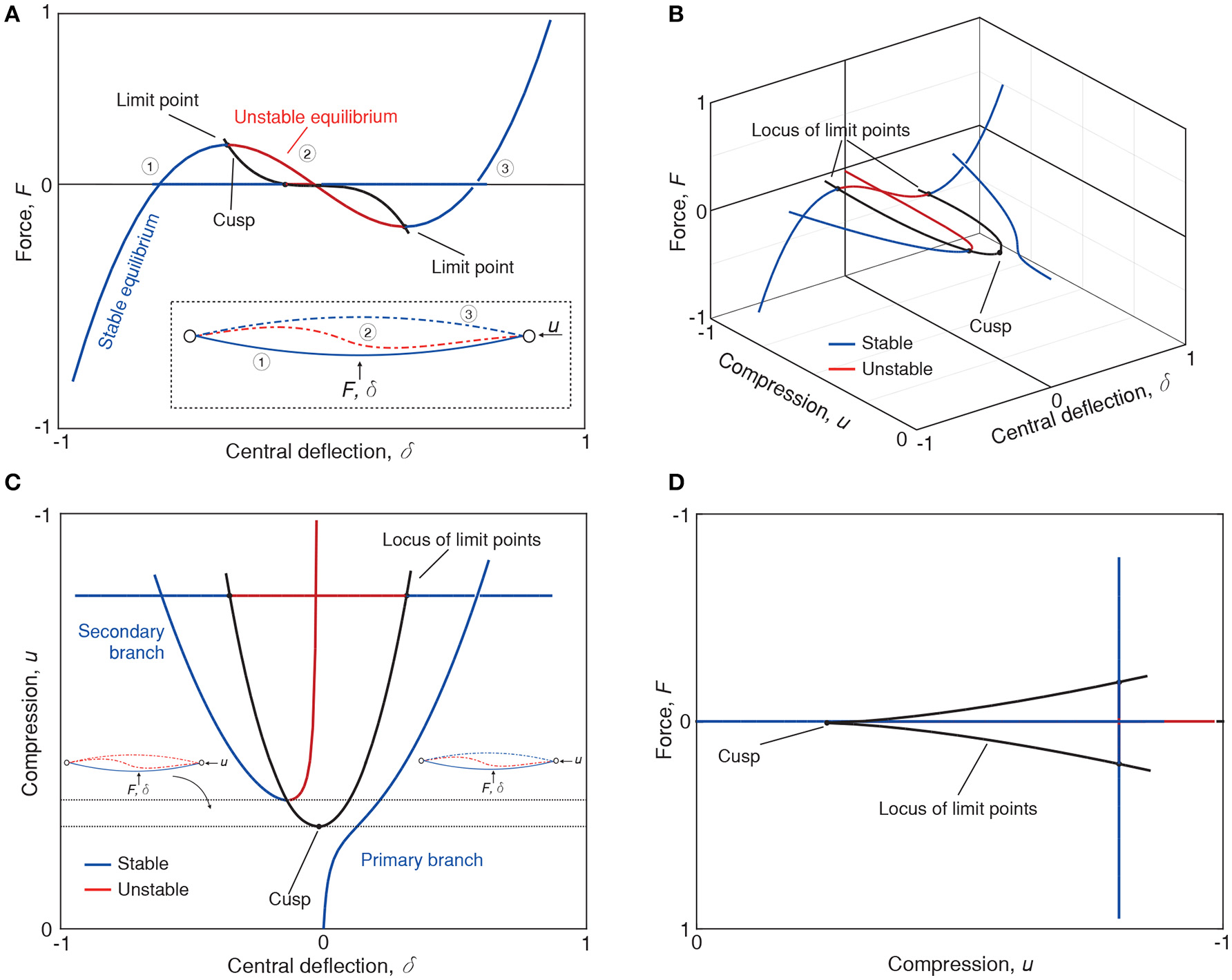
Figure 19. (A) Equilibrium path of force (F) vs. central deflection (δ). (B) Compression-central deflection-force space showing a broken pitchfork and the locus of limit points of the snap-through curve. (C,D) Show the locus of limits point in central deflection-compression and compression-force space, respectively.

Compression levels required to produce any meaningful shape-change from δ to −δ are typically sufficient to cause snap-through at a symmetry-breaking bifurcation (see asymmetric red shape in Figure 19A). Figure 19B shows how the equilibrium path in the F vs. δ plane connects the two stable branches of the broken pitchfork. Figure 19B also shows how the limit points of the F vs. δ equilibrium path change as a function of the compressive displacement, u, via the black fold line.

Specifically, the fold line tracks the two limit points with respect to changes in the compressive displacement, u, thereby illustrating the border between stable and unstable equilibria. By reducing u, the two limit points of the equilibrium path in Figure 19A collide in a cusp singularity (see Figures 19C,D). This cusp singularity therefore determines the critical value of compression, u, at the onset of dynamic snap-through behavior [97]. Indeed, depending on the value of compression, u, three distinct types of post-buckling behavior can be observed when the transverse load, F, is applied:

1. For values of compression, u, greater than the limit point on the broken-away pitchfork branch, the structure snaps from its first stable shape to its second configuration, traversing the region of instability delimited by the fold line. A self-equilibrated second configuration exists (stable even when F is removed). The structure is said to be bistable.

2. Reducing the compression, u, into the region between the limit point on the broken-away pitchfork branch and the cusp singularity, allows the beam to traverse a region of instability when F is applied, thereby still exhibiting snap-through behavior. However, at these values of compression, it does not have a second stable configuration for F = 0. When the external force is removed, the strut then snaps back to its primary state. In other words it shows “super-elastic” monostability.

3. By decreasing the level of compression, u, even further the structure deforms non-linearly, displaying stiffness adaptation but without snap-through. It is then elastically monostable or simply stable.

The control of geometrical parameters, material properties and/or boundary conditions can be used to tailor the equilibrium manifolds and adapt the multistability of the system to specific working and environmental conditions. We now consider a practical example.

A passive adaptive air inlet can regulate the opening aperture of a connected duct by interacting with the fluid flow around it. As shown in Figure 20, the inlet comprises a deformable, glass-fiber panel poised in an open state. The panel has been buckled into the region between the limit point of the broken-away branch and the cusp (refer to the taxonomy above), making it monostable.

FIGURE 20

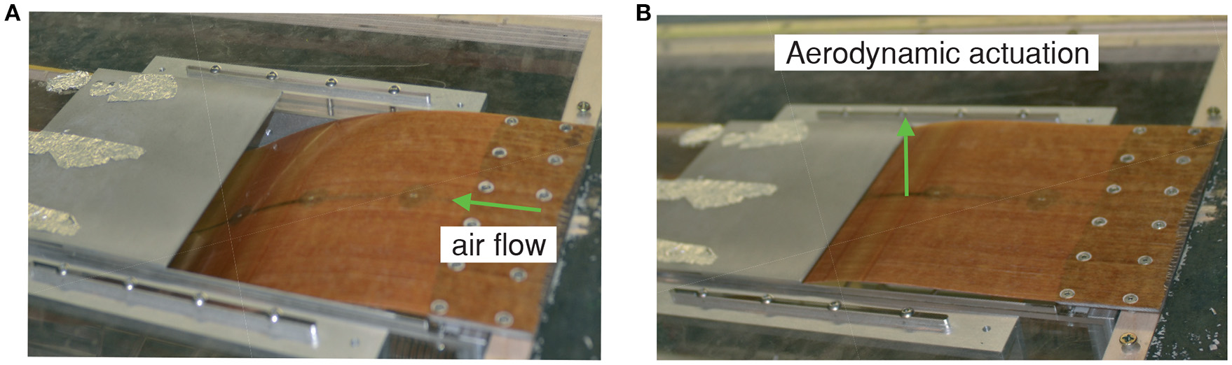
Figure 20. Adaptive air inlet demonstrator. (A) Open state. (B) Closed configuration.

As the airflow streaming over the panel accelerates into the connected duct, the decreasing pressure field creates an upwards force on the panel causing it to snap shut at a critical airspeed. If the airspeed is lowered beneath another threshold, the inlet automatically opens again. Unlike traditional shape-changing systems, the inlet does not rely on auxiliary devices for actuation. By increasing the amount of compression beyond the limit point on the broken-away path, the inlet can be transformed into a bistable structure that remains closed once the airflow is reduced. The greater the applied compression, the higher the airspeed required to actuate snap-through; the system's parameters can be tailored to meet specific operating requirements (see [98, 99] for further details).

This device has potential for engineering applications where cooling and drag reduction create competing design drivers. Examples include air inlets on cars or cooling ducts on jet engines, which use fresh-air cooling for reliable engine operation although this cooling induces a drag penalty. For additional engineering examples that use the non-linear taxonomy described above (see e.g., [100–107]) and references therein.

6.3. Buckling-Induced Auxetic Materials

The fact that materials exist with negative Poisson's ratio is not only intriguing but also of practical significance. So-called auxetic materials typically exhibit high energy absorption and fracture resistance, and have a broad range of practical applications from blast curtains and shock absorbers to running trainers and the ability to control waves (see for example [108–113] and references therein). Auxetic materials are known to occur naturally (various honeycomb structures for instance or even crumpled paper [113] but with recent technological advances in 3D printing they can also be readily manufactured. This ease of manufacture opens exciting new opportunities to tailor such materials, and work has exploded in this area. To show something of the flavor of this exciting new field, we now briefly outline two examples of auxetic behavior studied recently by the present authors, induced by local instabilities within the material's structure.

Experimental and numerical work led by Bertoldi et al. [111] has demonstrated how mechanical instabilities in periodic porous structures can lead to the dramatic reorganization of the material from the original configuration, giving rise to the auxetic possibilities. One widely studied structure involves the uni-axial loading of a square array of circular holes made of an elastomeric matrix, which can be readily manufactured using a 3D printer. The hexagonally-shaped sample shown in Figure 21 at the right is manufactured with an OBJET Connex 3D printer (Stratasys Ltd., USA), a machine that employs PolyJet Matrix Technology to dispense material—in this case Tango, a rubber-like elastomer—from designated micro-scale inkjet printing nozzles [114, 115]. When a compressive load is aligned with the square array, geometric reorganization is seen, as the elastic instability induces periodic deformation patterns of tessellating ∞-shaped voids. At the macroscale, this generates a non-linear auxetic response by the simulations shown in blue in Figure 21. Interestingly if our hexagonal specimen is rotated through 45°, so that the compressive load acts on a diamond arrangement of circular holes, the material response is close to that of classical linear elastic (non-auxetic) material (red line).

FIGURE 21

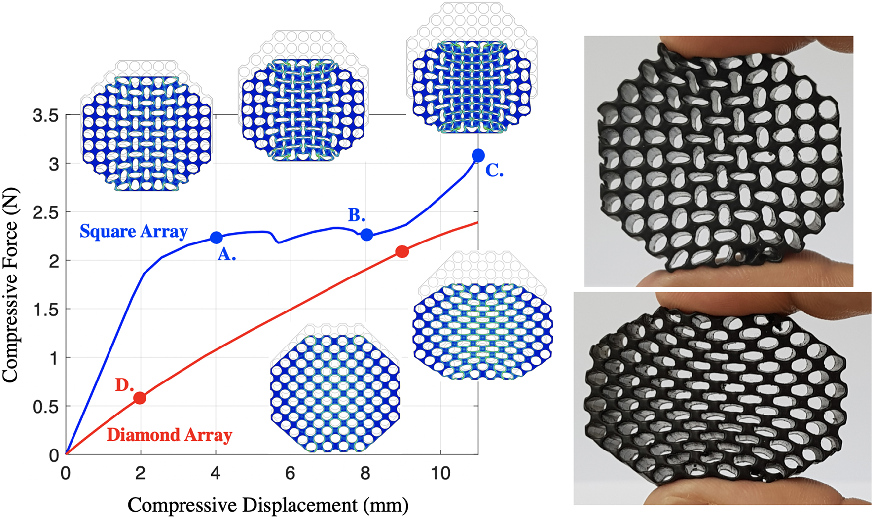
Figure 21. (Left) Shows 2D simulations of hexagonal lattices under different configurations (square and diamond) using ABAQUS. The geometry is discretized with 40,000 triangular elements, and model as linear elastic material under large deformation, strain and contact. (Right) Shows manufactured specimens in each of the configurations.

Most examples of auxetic behavior in the literature are based on re-entrant structures [108, 109, 113, 116], and we next briefly review a recent contribution [117] detailing a variant that allows phase transitions from auxetic to non-auxetic phases and vice versa, based on the unit cell shown in Figure 22. The cell comprises two back-to-back single degree-of-freedom arches with displacements measured by Q₁ and Q₂, linked by the linear spring of stiffness k [118]. Four different aspects of the full nonlinear response, including the important plot of load against its corresponding displacement of panel B, are given in Figure 23.

FIGURE 22

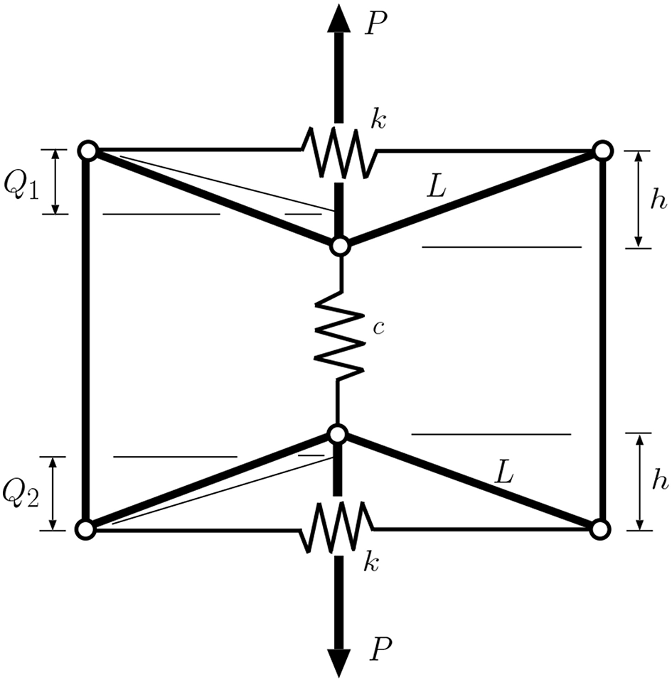
Figure 22. A new model for an auxetic cell, depicted in the unloaded state where P = 0 and Q₁ = Q₂ = h. The illustrated auxetic configuration becomes non-auxetic once the arms have passed through horizontal. Typically, the arches snap through in turn rather than simultaneously.

FIGURE 23

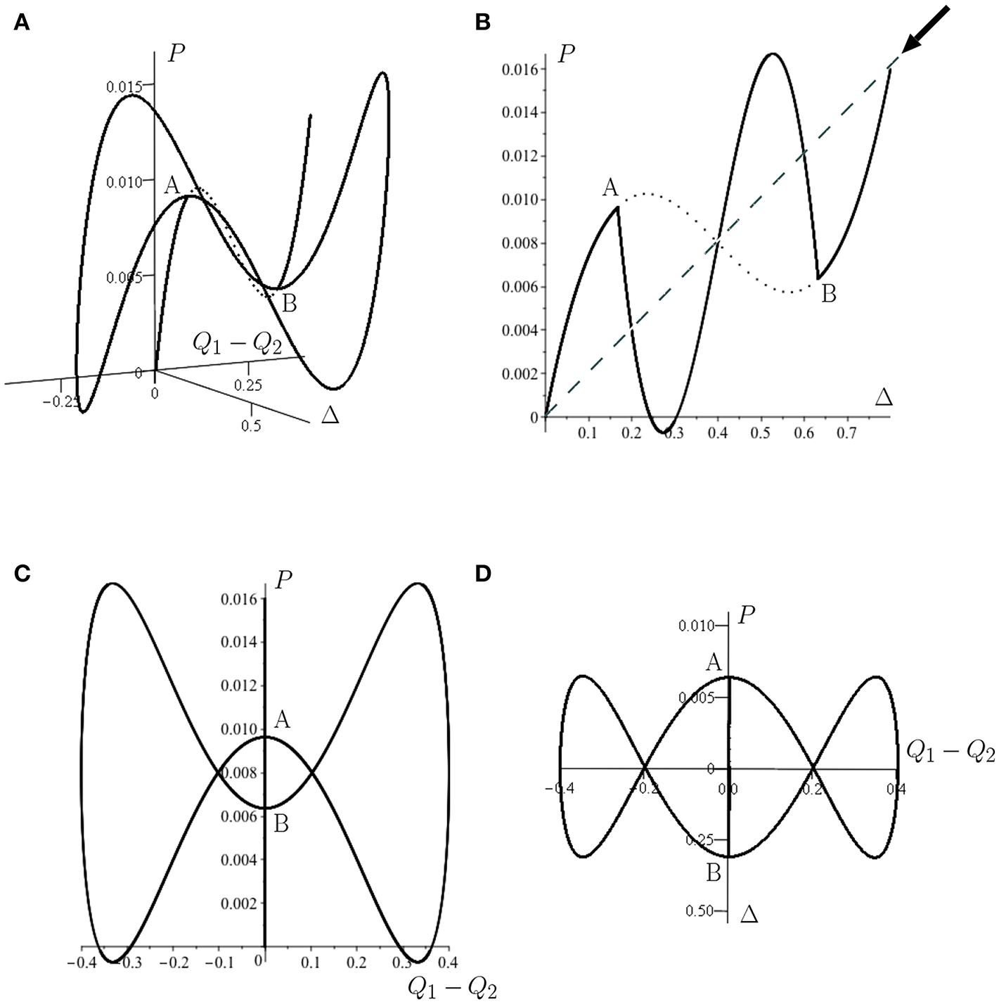
Figure 23. Response of the cell of Figure 22 for L = 1, h = 0.2, k = 1, and c = 0.02. Solid line depict stable equilibrium states under controlled stretch Δ, and the dotted line unstable states. (A) Three-dimensional plot of load P against its corresponding deflection Δ = 2h − Q₁ − Q₂, and the symmetry-breaking variable (Q₁ − Q₂). (B) Projection onto the P − Δ plane. (C) Projection onto the P − (Q₁ − Q₂) plane. (D) Projection onto plane perpendicular to the direction of the arrow in (B).

The continuous smooth curve replicates the response of a single arch [118], apart from the fact that under displacement control it goes unstable at bifurcation point A. Here the stable post-buckling solution becomes non-homogeneous, with displacement in one of the arches outpacing the other. This asymmetry continues until the first component passes through the horizontal and begins to stiffen, whereupon displacement in the other starts to take over. Symmetry is again restored at bifurcation B.

The absence of homogeneity in the natural loading path gives the potential for considerable complexity of response once cells are combined, as in Figure 24. The responses are shown in Figure 25. With a relatively modest extension of the single cell model, a complex tangle of stable and unstable equilibrium paths is generated. Further details can be found in Hunt and Dodwell [117].

FIGURE 24

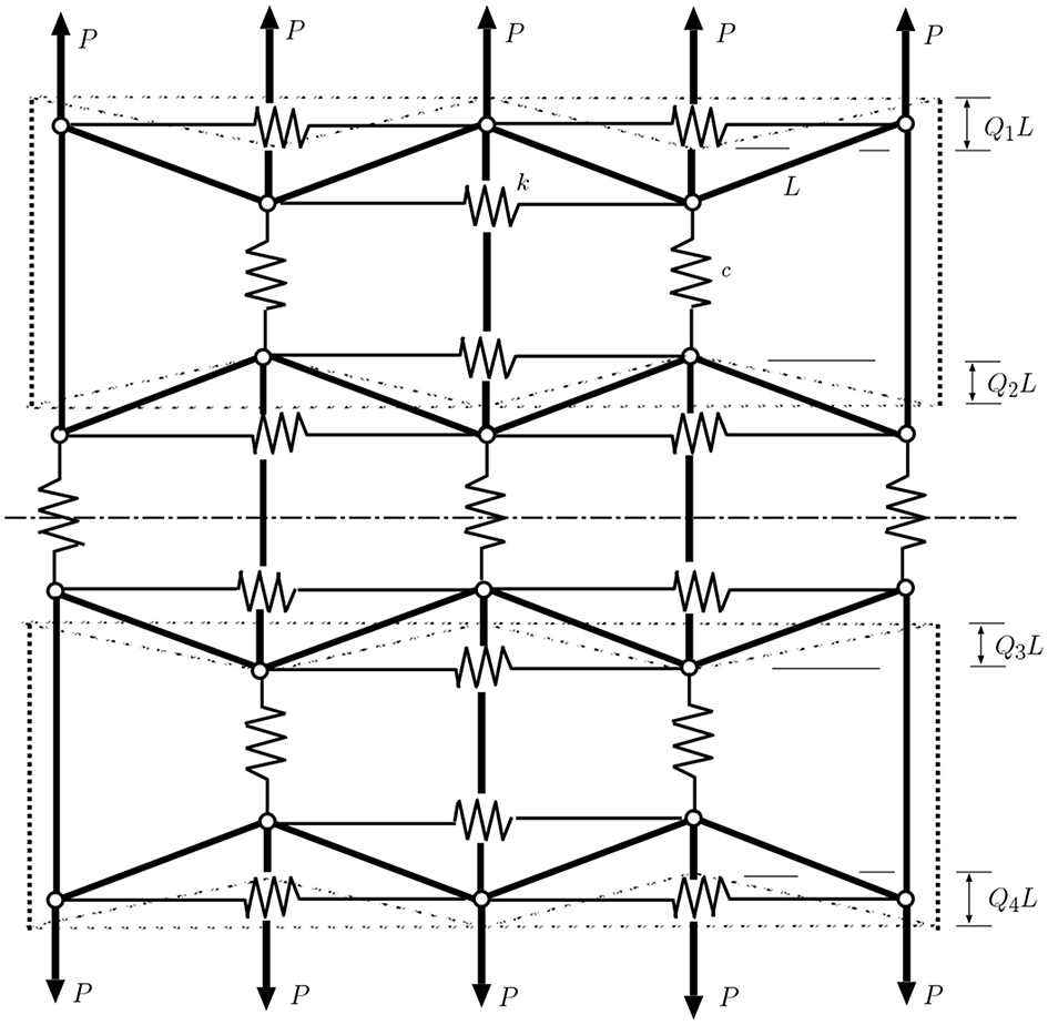
Figure 24. Combined cells of the form of Figure 22. With the centerline held stationary, displaced states are shown dashed. We refer to this configuration as a three-tier system, with four effective degrees-of-freedom Q_i, i = 1…4.

FIGURE 25

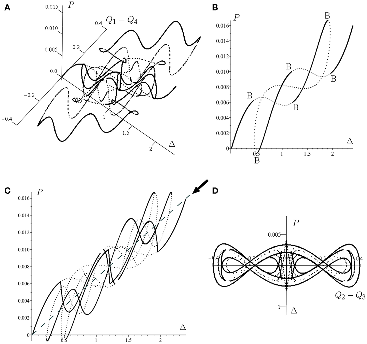
Figure 25. Response of the three-tier system of Figure 24, for L = 1, h = 0.2, k = 0.5, and c = 0.02. (A) Load P plotted against its corresponding deflection Δ and the symmetry-breaking variable (Q₁ − Q₄). (B) Symmetric solutions for which Q₁ = Q₄ and Q₂ = Q₃. (C) Projection of (A) on to the P − Δ plane. (D) Projection on to plane perpendicular to the direction of the arrow in (C).

7. Conclusion

This theme issue focuses on the notion of stability in a variety of different contexts, both mathematical and practical. It could be argued that there is no more classical context in which one thinks of stability than structural engineering. It is fundamentally the job of the structural engineer to avoid buckling, failure or collapse. This paper takes a slightly different point of view on the topic. We focus on emerging ideas of elastic stability and post-instability behavior of structures that fail subcritically, via irreversible jumps in energy. Such problems are of current interest for at least three reasons.

First and foremost, because of their sensitivity to shocks and imperfections, there is difficulty in certifying such structures for safety. We have argued that despite over 70 years since Koiter's pioneering work, a robust methodology for analyzing the stability of such structures has yet to emerge. We have promoted here a promising line of attack, based on the Maxwell equal energy criterion and the concept of the mountain pass, as well as emerging ideas on how such ideas might be applied experimentally. However, there remains much to be done before such ideas can provide a practical assessment and design tool. It is also interesting to note how the method relies on understanding the structure of unstable, localized post-buckling paths, which form the energy barriers or basin boundaries of the problem. In that sense, there is a strong connection to other active areas of stability-related research; tipping points in natural systems (see e.g., [119]), and transition to turbulence in pipe flow and related fluid-dynamic problems (see e.g., [120]).

Second, the structural engineering domain is changing. Across numerous lengthscales, there is a quest for ever more lightweight structures. It could be said that the revolution in composites and other nano-structured materials has been threatening to revolutionize just about the whole of the built environment for almost 50 years. Yet, despite the huge investment within academia and industry, why are we not yet seeing carbon fiber motor cars come off the production line, wholly composite airplanes in our airports, or fiber-reinforced polymer buildings being constructed en masse? There are doubtless a range of reasons for this slow penetration of composite technologies, and as most disruptive technologies, the revolution may actually be just around the corner. Nevertheless, we would argue that one of the bottlenecks still to be overcome, is that we do not understand how such structures fail. Most lightweight structures are optimized for strength, but such optimization typically leads to subcritical failure modes (see e.g., [28]). But, for structures made from composite materials, to the uncertainty and sensitivity of classical steel and concrete structures that buckle subcritically, we have additional complexities of anisotropy, internal micro-structural lengthscales and buried failures, cracks or delaminations that are hard to characterize and inspect. We have also seen, through the example of an auxetic material, that the distinction between materials and structures is fundamentally being blurred. It would seem then, the seeds of the robust methodology we have been trying to sow in this article are more important now than ever, if the true potential of nano-structured materials is to be realized in the built environment. We hope that future researchers may be inspired to water these seeds.

Finally, there is the point of view that we have been also trying to promote in this article that instability is not necessarily a bad thing. We have highlighted three areas of possible engineering exploitation of non-reversible structural instability. More generally though, we are quite used to the notion of things that snap and pop into instability. These include the pressure required to depress the keys on a computer keyboard being controlled by dome buckling, to old-fashioned bi-metallic strips being used to control switches, as in a motor car indicator light. Crash barriers and crumple zones also exploit the idea that elastic deformation of a subcritical structure can lead to transfer of significant amounts of energy into permanent plastic deformation. Origami also provides an inspiration to engineers in how small energy barriers need to be overcome in order to fold (or unfold) a structure into a new shape (see e.g., [121–123]). Most interestingly, there is great potential to draw inspiration from biology. Irreversible transitions are the norm in biology, for example in cell division, cell polarity formation and most morphogenesis problems. Although such processes are often controlled by genes and other signaling proteins, there is an increasing body of work that looks at the biomechanics of such transitions. Indeed, at many different lengthscales, processes that are crucial to development, or to the maintenance of an organism or ecosystem require sudden, irreversible response to continuous variation of external conditions. It is easy to think of examples like the springing of a Venus fly trap, or the opening of seed pods that can easily be regarded as buckling events of the nature described in this paper.

Clearly, there remain many lessons that engineers and designers need to learn by taking inspiration from the natural world. Not least among such lessons, as we seek to build a more resilient world in the face of global change, must surely be that there need not necessarily be anything to fear from an instability. Not only are sudden irreversible instabilities not necessarily to be feared, they can in fact be designed to be exploited for the greater good. Happy catastrophes indeed!

Data Availability

All data generated for this study can be found in the manuscript and/or supplementary material.

Author Contributions

All authors listed have made a substantial, direct and intellectual contribution to the work, and approved it for publication.

Funding

TD was funded by the Alan Turing Institute under a Turing Fellowship [Grant No. EP/N510129/1]. RG was funded by the Royal Academy of Engineering under the Research Fellowship scheme [Grant No. RF\201718\17178]. AP was funded by the UK Engineering and Physical Sciences Research Council under an Early Career Research Fellowship [Grant No. EP/M013170/1]. RN was funded by the UK Engineering and Physical Sciences Research Council [Grant No. EP/N509619/1].

Conflict of Interest Statement

The authors declare that the research was conducted in the absence of any commercial or financial relationships that could be construed as a potential conflict of interest.

Acknowledgments

The authors acknowledge useful conversations with D. Avitabile, G. J. Lord, J. Sieber, and J. M. T. Thompson.

Footnotes

1. ^The comma notation is used throughout to denote differentials with respect to subscripted variables

References

1. Budiansky B, Hutchinson JW. Buckling: progress and challenge. In: Besseling JF, van der Heijden AMJ, editors. Trends in Solid Mechanics 1979. Proceedings of the Symposium Dedicated to the 65th Birthday of W. T. Koiter. Delft: Delft University Press (1979).

Google Scholar

2. Hutchinson JW, Thompson JMT. Imperfections and energy barriers in shell buckling. Int J Solids Struct. (2018) 148:157–68. doi: 10.1016/j.ijsolstr.2018.01.030

CrossRef Full Text | Google Scholar

3. Reis PM. A perspective on the revival of structural (in)stability with novel opportunities for function: from Buckliphobia to Buckliphilia. J Appl Mech Trans ASME. (2015) 82:111001. doi: 10.1115/1.4031456

CrossRef Full Text | Google Scholar

4. Zeeman EC. Catastrophe theory. Sci Am. (1976) 65–70:75–83. doi: 10.1038/scientificamerican0476-65

CrossRef Full Text | Google Scholar

5. Thompson JMT. Catastrophe theory in mechanics: progress or digression. J Struct Mech. (1982) 10:167–75. doi: 10.1080/03601218208907408

CrossRef Full Text | Google Scholar

6. Wadee MA, Champneys AR. Fail safe or fail dangerous? In: Parc S, editor. 50 Visions of Mathematics. London: Oxford University Press (2014). p. 163–7.

Google Scholar

7. Thompson JMT, Hunt GW. A General Theory of Elastic Stability. London: John Wiley & Sons (1973).

Google Scholar

8. Arbocz J, Ho JMAM. Collapse of axially compressed cylindrical shells with random imperfections. AIAA J. (1991) 29:2247–56. doi: 10.2514/3.10866

CrossRef Full Text | Google Scholar

9. Elishakoff I, Li Y, Starnes JH Jr. Nonclassical Problems in the Theory of Elastic Stability. Cambridge: Cambridge University Press (2001).

Google Scholar

10. Croll JGA, Batista RC. Explicit lower bounds for the buckling of axially loaded cylinders. Int J Mech Sci. (1981) 23:331–43. doi: 10.1016/0020-7403(81)90063-1

CrossRef Full Text | Google Scholar

11. Thompson JMT, Sieber J. Shock-sensitivity in shell-like structures: with simulations of spherical shell buckling. Int J Bifurcation Chaos. (2015) 26:1630003. doi: 10.1142/S0218127416300032

CrossRef Full Text | Google Scholar

12. Kreilos T, Schneider TM. Fully localized post-buckling states of cylindrical shells under axial compression. Proc R Soc A Math Phys Eng Sci. (2017) 473:20170177. doi: 10.1098/rspa.2017.0177

PubMed Abstract | CrossRef Full Text | Google Scholar

13. Koiter WT. On the Stability of Elastic Equilibrium. Technische Hogeschool (Technological University of Delft), 1945, Delft, Netherlands (1967).

Google Scholar

14. Riks E. An incremental approach to the solution of snapping and buckling problems. Int J Solids Struct. (1979) 15:529–51. doi: 10.1016/0020-7683(79)90081-7

CrossRef Full Text | Google Scholar

15. Crisfield MA. A fast incremental/iterative solution procedure that handles “snap-through”. Comput Struct. (1981) 13:55–62. doi: 10.1016/0045-7949(81)90108-5

CrossRef Full Text | Google Scholar

16. Doedel EJ, Champneys AR, Fairgrieve TF, Kuznetsov YA, Sandstede B, Wang X. AUTO 97: Continuation and Bifurcation Software for Ordinary Differential Equations (With HomCont) (1998).

Google Scholar

17. Eriksson A. Structural instability analyses based on generalised path-following. Comput Meth Appl Mech Eng. (1998) 156:45–74. doi: 10.1016/S0045-7825(97)00200-4

CrossRef Full Text | Google Scholar

18. Groh RMJ, Avitabile D, Pirrera A. Generalised path-following for well-behaved nonlinear structures. Comput Meth Appl Mech Eng. (2018) 331:394–426. doi: 10.1016/j.cma.2017.12.001

CrossRef Full Text | Google Scholar

19. Castro SGP, Zimmermann R, Arbelo MA, Khakimova R, Hilburger MW, Degenhardt R. Geometric imperfections and lower-bound methods used to calculate knock-down factors for axially compressed composite cylindrical shells. Thin Walled Struct. (2014) 74:118–32. doi: 10.1016/j.tws.2013.08.011

CrossRef Full Text | Google Scholar

20. Lee A, López Jiménez F, Marthelot J, Hutchinson JW, Reis PM. The geometric role of precisely engineered imperfections on the critical buckling load of spherical elastic shells. J Appl Mech Trans ASME. (2016) 83:111005. doi: 10.1115/1.4034431

CrossRef Full Text | Google Scholar

21. Hunt GW, Peletier MA, Champneys AR, Woods PD, Wadee MA, Budd CJ, et al. Cellular buckling in long structures. Nonlinear Dyn. (2000) 21:3–29. doi: 10.1023/A:1008398006403

CrossRef Full Text | Google Scholar

22. Riks E. The application of Newton's method to the problem of elastic stability. J Appl Mech Trans ASME. (1971) 39:1060–5. doi: 10.1115/1.3422829

CrossRef Full Text | Google Scholar

23. Hunt GW. An algorithm for the nonlinear analysis of compound bifurcation. Phil Trans R Soc A Math Phys Eng Sci. (1981) 300:443–71. doi: 10.1098/rsta.1981.0075

CrossRef Full Text | Google Scholar

24. Koiter WT. The nonlinear buckling problem of a complete spherical shell under uniform external pressure. Proc Kon Ned Ak Wet. (1969) B72:40–123.

Google Scholar

25. Budd CJ, Hunt GW, Kuske R. Asymptotics of cellular buckling close to the Maxwell load. Proc R Soc A Math Phys Eng Sci. (2001) 457:2935–64. doi: 10.1098/rspa.2001.0843

CrossRef Full Text | Google Scholar

26. Kerr AD. On thermal buckling of straight railroad tracks and the effect of track length on track response. Rail Int. (1979) 9:759–68.

Google Scholar

27. Wadee MA, Hunt GW, Peletier MA. Kink band instability in layered structures. J Mech Phys Solids. (2004) 52:1071–91. doi: 10.1016/j.jmps.2003.09.026

CrossRef Full Text | Google Scholar

28. Hunt GW. Reflections and symmetries in space and time. IMA J Appl Math. (2011) 76:2–26. doi: 10.1093/imamat/hxq063

CrossRef Full Text | Google Scholar

29. Zhu E, Mandal P, Calladine CR. Buckling of thin cylindrical shells: An attempt to resolve a paradox. Int J Mech Sci. (2002) 44:1583–601. doi: 10.1016/S0020-7403(02)00065-6

CrossRef Full Text | Google Scholar

30. Elishakoff I. Probabilistic resolution of the twentieth century conundrum in elastic stability. Thin Walled Struct. (2012) 59:35–57. doi: 10.1016/j.tws.2012.04.002

CrossRef Full Text | Google Scholar

31. Yamaki N. Elastic Stability of Circular Cylindrical Shells. Elsevier (1984).

Google Scholar

32. Hunt GW, Bolt HM, Thompson JMT. Structural localization phenomena and the dynamical phase-space analogy. Proc R Soc A Math Phys Eng Sci. (1989) 425:245–67. doi: 10.1098/rspa.1989.0105

CrossRef Full Text | Google Scholar

33. Hunt GW, Lucena Neto E. Localized buckling in long axially-loaded cylindrical shells. J Mech Phys Solids. (1991) 39:881–94. doi: 10.1016/0022-5096(91)90010-L

CrossRef Full Text | Google Scholar

34. Hunt GW, Lord GJ, Champneys AR. Homoclinic and heteroclinic orbits underlying the post-buckling of axially-compressed cylindrical shells. Comput Meth Appl Mech Eng. (1999) 170:239–51. doi: 10.1016/S0045-7825(98)00197-2

CrossRef Full Text | Google Scholar

35. Horák J, Lord GJ, Peletier MA. Cylinder buckling: the mountain pass as an organizing center. SIAM J Appl Math. (2006) 66:1793–824. doi: 10.1137/050635778

CrossRef Full Text | Google Scholar

36. Hutchinson JW. Buckling of spherical shells revisited. Proc R Soc A Math Phys Eng Sci. (2016) 472:20160577. doi: 10.1098/rspa.2016.0577

CrossRef Full Text | Google Scholar

37. Beaty D. A Theoretical and Experimental Study of the Stability of Thin Elastic Spherical Shells. Michigan, MI: University of Michigan (1962).

Google Scholar

38. Walker AC. An analytical study of the rotationally symmetric non-linear buckling of a complete spherical shell under external pressure. Int J Mech Sci. (1968) 10:695–710. doi: 10.1016/0020-7403(68)90084-2

CrossRef Full Text | Google Scholar

39. Hunt GW, Lucena Neto E. Maxwell critical loads for axially loaded cylindrical shells. J Appl Mech Trans ASME. (1993) 60:702–6. doi: 10.1115/1.2900861

CrossRef Full Text | Google Scholar

40. Hunt GW, Lord GJ, Peletier MA. Cylindrical shell buckling: a characterization of localization and periodicity. Discrete Contin Dyn Syst Ser B. (2003) 3:505–18. doi: 10.3934/dcdsb.2003.3.505

CrossRef Full Text | Google Scholar

41. Golubitsky M, Stewart I, Schaeffer D. Singularities and Groups in Bifurcation Theory. Vol. 2. New York, NY: Springer (1998).

Google Scholar

42. Kuznetsov Y. Elements of Applied Bifurcation Theory. 3rd ed. New York, NY: Springer (2004).

Google Scholar

43. Haragus M, Iooss G. Local Bifurcations, Center Manifolds and Normal Forms in Infinite-Dimensional Dynamical Systems. New York, NY: Springer (2011).

Google Scholar

44. Keller HB. Lectures on Numerical Methods in Bifurcation Problems. Berlin: Springer (1986).

Google Scholar

45. Doedel EJ, Oldeman BE. AUTO-07P: Continuation and Bifurcation Software for Ordinary Differential Equations. Montreal, QC (2011).

Google Scholar

46. Sewell MJ. On the connection between stability and the shape of the equilibrium surface. J Mech Phys Solids. (1966) 14:203–30. doi: 10.1016/0022-5096(66)90030-5

CrossRef Full Text | Google Scholar

47. Ahmad S, Irons BM, Zienkiewicz OC. Analysis of thick and thin shell structures by curved finite elements. Int J Numer Methods Eng. (1970) 2:419–51. doi: 10.1002/nme.1620020310

CrossRef Full Text | Google Scholar

48. Reissner E. On the theory of bending of elastic plates. J Math Phys. (1944) 23:184–91. doi: 10.1002/sapm1944231184

CrossRef Full Text | Google Scholar

49. Payette GS, Reddy JN. A seven-parameter spectral/hp finite element formulation for isotropic, laminated composite and functionally graded shell structures. Comput Meth Appl Mech Eng. (2014) 278:664–704. doi: 10.1016/j.cma.2014.06.021

CrossRef Full Text | Google Scholar

50. Bathe KJ. Finite Element Procedures. 1st ed. Watertown, MA: TBS (2007).

Google Scholar

51. Pomeau Y. Front motion, metastability and subcritical bifurcations in hydrodynamics. Phys D. (1986) 23:3–11. doi: 10.1016/0167-2789(86)90104-1

CrossRef Full Text | Google Scholar

52. Knobloch E. Spatial localization in dissipative systems. Annu Rev Condens Matter Phys. (2015) 6:325–59. doi: 10.1146/annurev-conmatphys-031214-014514

CrossRef Full Text | Google Scholar

53. Groh RMJ, Pirrera A. On the role of localizations in buckling of axially compressed cylinders. Proc R Soc A Math Phys Eng Sci. (2019) 475:20190006. doi: 10.1098/rspa.2019.0006

PubMed Abstract | CrossRef Full Text | Google Scholar

54. Zeeman EC. Catastrophe Theory: Selected Papers, 1972–1977. London: Addison-Wesley (1977).

Google Scholar

55. Wadee MA, Edmunds R. Kink band propagation in layered structures. J Mech Phys Solids. (2005) 53:2017–35. doi: 10.1016/j.jmps.2005.04.005

CrossRef Full Text | Google Scholar

56. Wadee MA, Gardner L. Cellular buckling from mode interaction in I-beams under uniform bending. Proc R Soc A Math Phys Eng Sci. (2012) 468:245–68. doi: 10.1098/rspa.2011.0400

CrossRef Full Text | Google Scholar

57. Wadee MA, Bai L. Cellular buckling in I-section struts. Thin Walled Struct. (2014) 81:89–100. doi: 10.1016/j.tws.2013.08.009

CrossRef Full Text | Google Scholar

58. Bai L, Wang F, Wadee MA, Yang J. Nonlinear mode interaction in equal-leg angle struts susceptible to cellular buckling. Proc R Soc A Math Phys Eng Sci. (2017) 473:20170583. doi: 10.1098/rspa.2017.0583

PubMed Abstract | CrossRef Full Text | Google Scholar

59. Yu J, Wadee MA. Mode interaction in triple-bay prestressed stayed columns. Int J Nonlinear Mech. (2017) 88:47–66. doi: 10.1016/j.ijnonlinmec.2016.10.012

CrossRef Full Text | Google Scholar

60. Ambrosetti A, Rabinowitz PH. Dual variational methods in critical point theory and applications. J Funct Anal. (1973) 14:349–81. doi: 10.1016/0022-1236(73)90051-7

CrossRef Full Text | Google Scholar

61. Henkelman G, Uberuaga BP, Jónsson H. A climbing image nudged elastic band method for finding saddle points and minimum energy paths. J Chem Phys. (2000) 113:9901. doi: 10.1063/1.1329672

CrossRef Full Text | Google Scholar

62. Henkelman G, Jónsson H. A dimer method for finding saddle points on high dimensional potential surfaces using only first derivatives. J Chem Phys. (1999) 111:7010. doi: 10.1063/1.480097

CrossRef Full Text | Google Scholar

63. Fischer A, Karplus M. Conjugate peak refinement–an algorithm for finding reaction paths and accurate transition-states in systems with many degrees of freedom. Chem Phys Lett. (1992) 194:252–61. doi: 10.1016/0009-2614(92)85543-J

CrossRef Full Text | Google Scholar

64. Bonfanti S, Kob W. Methods to locate saddle points in complex landscapes. J Chem Phys. (2017) 147:204104. doi: 10.1063/1.5012271

PubMed Abstract | CrossRef Full Text | Google Scholar

65. Thompson JMT. Advances in shell buckling: theory and experiments. Int J Bifurcation Chaos. (2015) 25:1530001. doi: 10.1142/S0218127415300013

CrossRef Full Text | Google Scholar

66. Lord GJ, Champneys AR, Hunt GW. Computation of homoclinic orbits in partial differential equations: an application to cylindrical shell buckling. SIAM J Sci Comput. (1999) 21:591–619. doi: 10.1137/S1064827597321647

CrossRef Full Text | Google Scholar

67. Virot E, Kreilos T, Schneider TM, Rubinstein SM. Stability landscape of shell buckling. Phys Rev Lett. (2017) 119:224101. doi: 10.1103/PhysRevLett.119.224101

PubMed Abstract | CrossRef Full Text | Google Scholar

68. Babcock CD, Sechler EE. The Effect of Initial Imperfections on the Buckling Stress of Cylindrical Shells. NASA TN D-2005. Pasadena, CA: California Institute of Technology (1963).

Google Scholar

69. Arbocz J. The Effect of General Imperfections on the Buckling of Cylindrical Shells. Pasadena, CA: California Institute of Technology (1968).

Google Scholar

70. Tennyson RC. Buckling modes of circular cylindrical shells under axial compression. AIAA J. (1969) 7:1481–7. doi: 10.2514/3.5419

CrossRef Full Text | Google Scholar

71. Hühne C, Rolfes R, Breitbach E, Teßler J. Robust design of composite cylindrical shells under axial compression—simulation and validation. Thin Walled Struct. (2008) 46:947–62. doi: 10.1016/j.tws.2008.01.043

CrossRef Full Text | Google Scholar

72. Hilburger MW. On the development of shell buckling knockdown factors for stiffened metallic launch vehicle cylinders. In: Proceedings of the 2018 AIAA/ASCE/AHS/ASC Structures, Structural Dynamics, and Materials Conference (Grapevine, TX) (2018).

Google Scholar

73. Wiebe R, Virgin LN. On the experimental identification of unstable static equilibria. Proc R Soc A Math Phys Eng Sci. (2016) 472:20160172. doi: 10.1098/rspa.2016.0172

PubMed Abstract | CrossRef Full Text | Google Scholar

74. Neville RM, Groh RMJ, Pirrera A, Schenk M. Shape control for experimental continuation. Phys Rev Lett. (2018) 120:254101. doi: 10.1103/PhysRevLett.120.254101

PubMed Abstract | CrossRef Full Text | Google Scholar

75. Groh RMJ, Neville RM, Pirrera A, Schenk M. Virtual testing of experimental continuation. ArXiv e-prints (2018).

Google Scholar

76. Neville RM, Groh RMJ, Pirrera A, Schenk M. Quasi-static experimental path-following. In: Proc. AIAA SciTech 2019 (San Diego, CA) (2019).

Google Scholar

77. Eßlinger M, Geier B. Gerechnete Nachbeullasten als untere Grenze der experimentellen axialen Beullasten von Kreiszylindern. Der Stahlbau. (1972) 21:353–60.

Google Scholar

78. Weingarten VI, Morgan EJ, Seide P. Elastic stability of thin-walled cylindrical and conical shells under axial compression. AIAA J. (1965) 3:500–5. doi: 10.2514/3.2893

CrossRef Full Text | Google Scholar

79. Degenhardt R, Kling A, Bethge A, Orf J, Kärger L, Zimmermann R, et al. Investigations on imperfection sensitivity and deduction of improved knock-down factors for unstiffened CFRP cylindrical shells. Compos Struct. (2010) 92:1939–46. doi: 10.1016/j.compstruct.2009.12.014

CrossRef Full Text | Google Scholar

80. Meurer A, Kriegesmann B, Dannert M, Rolfes R. Probabilistic perturbation load approach for designing axially compressed cylindrical shells. Thin Walled Struct. (2016) 107:648–56. doi: 10.1016/j.tws.2016.07.021

CrossRef Full Text | Google Scholar

81. Wang B, Hao P, Li G, Fang Y, Wang X, Zhang X. Determination of realistic worst imperfection for cylindrical shells using surrogate model. Struct Multidiscip Optim. (2013) 48:777–94. doi: 10.1007/s00158-013-0922-9

CrossRef Full Text | Google Scholar

82. Fan H. Critical buckling load prediction of axially compressed cylindrical shell based on non-destructive probing method. Thin Walled Struct. (2019) 139:91–104. doi: 10.1016/j.tws.2019.02.034

CrossRef Full Text | Google Scholar

83. Hafez HH, Temple MC, Ellis JS. Pretensioning of single-crossarm stayed columns. J Struct Div ASCE. (1979) 105:359–75.

Google Scholar

84. Saito D, Wadee MA. Post-buckling behaviour of prestressed steel stayed columns. Eng Struct. (2008) 30:1224–39. doi: 10.1016/j.engstruct.2007.07.012

CrossRef Full Text | Google Scholar

85. Osofero AI, Wadee MA, Gardner L. Experimental study of critical and post-buckling behaviour of prestressed stayed columns. J Constr Steel Res. (2012) 79:226–41. doi: 10.1016/j.jcsr.2012.07.013

CrossRef Full Text | Google Scholar

86. Saito D, Wadee MA. Numerical studies of interactive buckling in prestressed steel stayed columns. Eng Struct. (2009) 31:432–43. doi: 10.1016/j.engstruct.2008.09.008

CrossRef Full Text | Google Scholar

87. Yu J, Wadee MA. Optimal prestressing of triple-bay prestressed stayed columns. Structures. (2017) 12:132–44. doi: 10.1016/j.istruc.2017.09.001

CrossRef Full Text | Google Scholar

88. Lapira L, Wadee MA, Gardner L. Stability of multiple-crossarm prestressed stayed columns with additional stay systems. Structures. (2017) 12:227–41. doi: 10.1016/j.istruc.2017.09.010

CrossRef Full Text | Google Scholar

89. Wadee MA, Gardner L, Hunt TA. Buckling mode interaction in prestressed stayed columns. Proc Inst Civil Eng Struct Build. (2013) 166:403–12. doi: 10.1680/stbu.12.00080

CrossRef Full Text | Google Scholar

90. Queheillalt DT, Wadley HNG. Cellular metal lattices with hollow trusses. Acta Mater. (2005) 53:303–13. doi: 10.1016/j.actamat.2004.09.024

CrossRef Full Text | Google Scholar

91. Zschernack C, Wadee MA, Völlmecke C. Nonlinear buckling of fibre-reinforced unit cells of lattice materials. Compos Struct. (2016) 136:217–28. doi: 10.1016/j.compstruct.2015.09.059

CrossRef Full Text | Google Scholar

92. Schenk M, Guest SD. On zero stiffness. Proc Inst Mech Eng C J Mech Eng Sci. (2014) 228:1701–14. doi: 10.1177/0954406213511903

CrossRef Full Text | Google Scholar

93. Virgin LN, Davis RB. Vibration isolation using buckled struts. J Sound Vibr. (2003) 260:965–73. doi: 10.1016/S0022-460X(02)01177-X

CrossRef Full Text | Google Scholar

94. Thill C, Etches J, Bond I, Potter K, Weaver PM. Morphing skins. Aeronaut J. (2008) 112:117–39. doi: 10.1017/S0001924000002062

CrossRef Full Text | Google Scholar

95. Sun J, Guan Q, Liu Y, Leng J. Morphing aircraft based on smart materials and structures: a state-of-the-art review. J Intell Mater Sys Struct. (2016) 27:2289–312. doi: 10.1177/1045389X16629569

CrossRef Full Text | Google Scholar

96. Forterre Y, Skotheim JM, Dumais J, Mahadevan L. How the Venus flytrap snaps. Nature. (2005) 433:421–5. doi: 10.1038/nature03185

PubMed Abstract | CrossRef Full Text | Google Scholar

97. Danso LA, Karpov EG. Cusp singularity-based bistability criterion for geometrically nonlinear structures. Extreme Mech Lett. (2017) 13:135–40. doi: 10.1016/j.eml.2017.01.001

CrossRef Full Text | Google Scholar

98. Arena G, Groh RMJ, Brinkmeyer A, Theunissen R, Weaver PM, Pirrera A. Adaptive compliant structures for flow regulation. Proc R Soc A Math Phys Eng Sci. (2017) 473:20170334. doi: 10.1098/rspa.2017.0334

PubMed Abstract | CrossRef Full Text | Google Scholar

99. Arena G, Groh RMJ, Theunissen R, Weaver PM, Pirrera A. Design and testing of a passively adaptive inlet. Smart Mater Struct. (2018) 27:085019. doi: 10.1088/1361-665X/aacf79

CrossRef Full Text | Google Scholar

100. Kebadze E, Guest SD, Pellegrino S. Bistable prestressed shell structures. Int J Solids Struct. (2004) 41:2801–20. doi: 10.1016/j.ijsolstr.2004.01.028

CrossRef Full Text | Google Scholar

101. Diaconu CG, Weaver PM, Mattioni F. Concepts for morphing airfoil sections using bi-stable laminated composite structures. Thin Walled Struct. (2008) 46:689–701. doi: 10.1016/j.tws.2007.11.002

CrossRef Full Text | Google Scholar

102. Mattioni F, Weaver PM, Friswell M. Multistable composite plates with piecewise variation of lay-up in the planform. Int J Solids Struct. (2009) 46:151–64. doi: 10.1016/j.ijsolstr.2008.08.023

CrossRef Full Text | Google Scholar

103. Kuder IK, Arrieta AF, Raither WE, Ermanni P. Variable stiffness material and structural concepts for morphing applications. Prog Aerosp Sci. (2013) 63:33–55. doi: 10.1016/j.paerosci.2013.07.001

CrossRef Full Text | Google Scholar

104. Arrieta A, Bilgen O, Friswell MI, Ermanni P. Modelling and configuration control of wing-shaped bi-stable piezoelectric composites under aerodynamic loads. Aerosp Sci Technol. (2013) 29:453–61. doi: 10.1016/j.ast.2013.05.004

CrossRef Full Text | Google Scholar

105. Terwagne D, Brojan M, Reis PM. Smart morphable surfaces for aerodynamic drag control. Adv Mater. (2014) 26:6608–11. doi: 10.1002/adma.201401403

PubMed Abstract | CrossRef Full Text | Google Scholar

106. Emam S, Inman D. A review on bistable composite laminates for morphing and energy harvesting. Appl Mech Rev. (2015) 67:060803. doi: 10.1115/1.4032037

CrossRef Full Text | Google Scholar

107. Zirbel SA, Tolman KA, Trease BP, Howell LL. Bistable mechanisms for space applications. PLoS ONE. (2016) 11:e0168218. doi: 10.1371/journal.pone.0168218

PubMed Abstract | CrossRef Full Text | Google Scholar

108. Evans KE, Alderson A. Auxetic materials: functional materials and structures from lateral thinking. Adv Mater. (2000) 12:617–28. doi: 10.1002/(SICI)1521-4095(200005)12:9<617::AID-ADMA617>3.0.CO;2-3

CrossRef Full Text | Google Scholar

109. Evans KE, Alderson KL. Auxetic materials: the positive side of being negative. Eng Sci Educ J. (2000) 9:148–54. doi: 10.1049/esej:20000402

CrossRef Full Text | Google Scholar

110. Evans KE, Nkansah MA, Hutchinson IJ, Rogers SC. Molecular network design. Nature. (1991) 353:124. doi: 10.1038/353124a0

CrossRef Full Text | Google Scholar

111. Bertoldi K, Reis PM, Willshaw S, Mullin T. Negative Poisson's ratio behaviour induced by an elastic instability. Adv Mater. (2010) 22:361–6. doi: 10.1002/adma.200901956

CrossRef Full Text | Google Scholar

112. Overvelde JTB, Shan S, Bertoldi K. Compaction through buckling in 2D periodic, soft and porous structures: effect of pore shape. Adv Mater. (2012) 24:2337–42. doi: 10.1002/adma.201104395

PubMed Abstract | CrossRef Full Text | Google Scholar

113. Yang W, Li ZM, Shi W, Xie BH, Yang MB. Review on auxetic materials. J Mater Sci. (2004) 39:3269–79. doi: 10.1023/B:JMSC.0000026928.93231.e0

CrossRef Full Text | Google Scholar

114. Stratasys. PolyJet Multi-Material 3D Printing. Rehovot: Stratasys (2015).

Google Scholar

115. Sakhaei AH, Kaijima S, Lee TL, Tan YY, Dunn ML. Design and investigation of a multi-material compliant ratchet-like mechanism. Mech Mach Theory. (2018) 121:184–97. doi: 10.1016/j.mechmachtheory.2017.10.017

CrossRef Full Text | Google Scholar

116. Lakes RS. Foam structures with a negative Poisson's ratio. Science. (1987) 235:1038–40. doi: 10.1126/science.235.4792.1038

PubMed Abstract | CrossRef Full Text | Google Scholar

117. Hunt GW, Dodwell TJ. Complexity in phase transforming pin-jointed auxetic lattices. Proc R Soc A Math Phys Eng Sci. (2019) 475:20180720. doi: 10.1098/rspa.2018.0720

PubMed Abstract | CrossRef Full Text | Google Scholar

118. Thompson JMT, Hunt GW. Elastic Instability Phenomena. Chichester: John Wiley & Sons (1984).

Google Scholar

119. Thompson JMT, Sieber J. Climate tipping as a noisy bifurcation: a predictive technique. IMA J Appl Math. (2011) 76:27–46. doi: 10.1093/imamat/hxq060

CrossRef Full Text | Google Scholar

120. Kerswell RR. Recent progress in understanding the transition to turbulence in a pipe. Nonlinearity. (2005) 18:R17. doi: 10.1088/0951-7715/18/6/R01

CrossRef Full Text | Google Scholar

121. Schenk M, Guest SD. Geometry of miura-folded metamaterials. Proc Natl Acad Sci USA. (2013) 110:3276–81. doi: 10.1073/pnas.1217998110

PubMed Abstract | CrossRef Full Text | Google Scholar

122. Silverberg JL, Evans AA, McLeod L, Hayward RC, Hull T, Santangelo CD, et al. Using origami design principles to fold reprogrammable mechanical metamaterials. Science. (2014) 345:647–50. doi: 10.1126/science.1252876

PubMed Abstract | CrossRef Full Text | Google Scholar

123. Liu K, Paulino GH. Nonlinear mechanics of non-rigid origami: an efficient computational approach. Proc Roy Soc A. (2017) 473:1–28. doi: 10.1098/rspa.2017.0348

PubMed Abstract | CrossRef Full Text | Google Scholar