Detection of Spatio-Temporal Recurrent Patterns in Dynamical Systems

1. Introduction

Complex dynamical systems arise in many fields of science, e.g., in biology, physics, climatology, and engineering. Those are systems exhibiting nonlinear, non-stationary, and possibly even chaotic behavior which is generally difficult to model or analyze. Several dynamical systems are also characterized by a well defined spatial organization (like the human brain for instance), and to properly describe their dynamics, one must take into account both their spatial and temporal properties. A way to achieve this is by analyzing the spatio-temporal data that can be observed from the complex system. In this respect, an important observation is that dynamical systems tend to return to former states, and this recurrence can be recognized as a fundamental characteristic of many dynamical systems [1] which can be used to study their behavior. Eckmann et al. introduced the method of Recurrence Plots (RPs) to visualize and quantify the recurrent behavior of the phase-space trajectory of a dynamical system [2]. Depending on the distance measure used, RPs are known to characterize the underlying trajectory up to isometry, and an underlying time series up to a sign choice under mild conditions [3, 4]. Once the RP of a dynamical system is obtained, Recurrence Quantification Analysis (RQA) [5] can be employed to further quantify the properties of its recurrent behavior. RPs have been successfully used in numerous fields of research such as astrophysics, earth sciences, biology and physiology, and engineering [1].

Originally, RPs were developed for the study of phase-space trajectories, or for uni-variate time series through time-delay embeddings. Several extensions have been proposed to deal with multi-variate time series data and with spatio-temporal processes which can also exhibit typical recurrent structures of interest (the interested reader is invited to read section 2 for more background information about multi-variate and spatial recurrence plots). Those approaches for multi-variate RPs and their accompanying RQA generally exploit the whole record of spatio-temporal data observed from the complex dynamical system under investigation; they do not aim to find a subset on which to perform a more focused and informative analysis. However, for a given system with an arbitrary spatial or geometric structure, recurrence (perceived as quasi-periodic repetitive patterns) may occur in localized regions of this structure only (limited over space), and may last for just a limited time (relative to the overall time span of the data). Not focusing on such most informative spatio-temporal regions of interest in the data, may hinder the identification and characterization of complex dynamics with RQA, as relevant information becomes obscured by getting drowned in uninformative data and noise. In addition, from a computational point of view, it is also inefficient to build RPs and perform RQA on complete multi-variate datasets if one is predominantly interested in spatio-temporally localized recurrences. We therefore argue that, before carrying out multi-variate RPs and RQA, it is important to first detect if, where, and when recurrence patterns are present and recognizable. This will allow one to select the spatial region(s) and time interval(s) of interest for performing a more efficient and accurate analysis of recurrence, leaving out much of the unwanted disinformation.

In this study, we propose a novel such framework for the detection of spatio-temporal recurrence in complex dynamical systems, This framework focuses on a specific type of recurrence, namely, recurrences from repetitive (relatively short lived) quasi-periodic oscillatory patterns, with a limited frequency bandwidth. This kind of recurrence is important in signal processing applications, especially in the field of medicine from which we shall present an example with real data. The framework (see Figure 1) is designed to work with spatial structures of arbitrary geometry (which can be graph-based and need not be confined to regular grids). It first uses Principal Component Analysis (PCA) to identify the points in the geometric structure associated with a local recurrent pattern, and then clusters those points to find the geometric regions where the recurrent patterns are located. In order to estimate the corresponding time interval of each recurrent pattern, a time windowing procedure is developed. The effectiveness of this method is illustrated with two numerical simulations. The practical relevance of the framework of this study is then demonstrated by means of an application with real data. In this application, the goal is to identify recurrence in atrial fibrillation (AF) propagation patterns in high-density contact mapping in a sheep model of acute AF. AF is a cardiac arrhythmia characterized by an irregular electrical activity in the atria, the upper chambers of the heart. AF may be driven by specific regions within the atria that spontaneously generate electrical activity in an uncoordinated way, or by self-perpetuating quasi-periodic re-entry patterns of propagation of electrical wave fronts, which may happen both globally (at the level of the whole atria), or locally (at the level of sub-regions of the atria). Therefore wave front propagation during AF is a complex phenomenon, which may be localized both in time and space, and which provides a natural application for the framework proposed in this study [6]. The results presented in this paper demonstrate the applicability and validity of the proposed framework for the detection of spatio-temporally localized recurrence in complex dynamical systems.

FIGURE 1

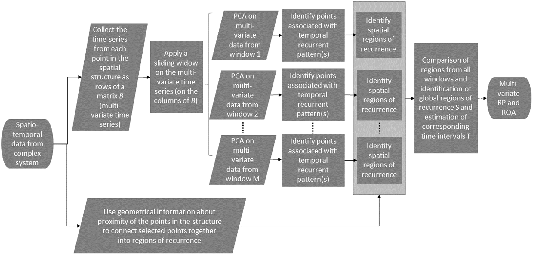
Figure 1. Schematic of the framework. Briefly, the time series associated with each point in the geometric structure are collected into a matrix B, which can be seen as a multi-variate time series. A sliding window is applied over the multi-variate time series, and each window is decomposed by means of PCA. The information from the PCA decomposition is used to retrieve the points in the structure associated with a temporal recurrent pattern. The geometric information about proximity of the points is then used to cluster together points of recurrence which are next to each other, and identify spatial regions of recurrence. Finally, the information from all windows is used to create global regions of recurrence and estimate their time intervals (spatio-temporal recurrence).

2. Background on Multi-Variate and Spatial Recurrence Plots

As mentioned in the Introduction, several extensions of RP and RQA have been proposed to deal with multi-variate time series data and with spatial data. Romano et al. [7] proposed to calculate RPs of multi-variate time series based on joint recurrence in phase space. This approach focuses on studying the phase synchronization of two bidirectionally coupled chaotic systems, depending on their coupling strength, and frequency mismatch. Nichols et al. [8] used RP and RQA for damage detection in structures, and they showed how it can be extended to include multi-variate observations coming from a spatially distributed network of sensors. The authors proposed a simple embedding procedure for multi-variate time series, in which each embedded vector is built by taking the samples from all sensors at a given time instant. We used a similar idea to generate multi-variate RPs in this study, as discussed in section 3.2.

When the focus is on spatial data structures characterized by high-dimension and geometric correlation patterns (different from time series data), traditional RP is limited in analyzing it, since recurrene may occur in any spatial direction (and not simply over time). In this respect, Vasconcelos et al. [9] investigated recurrence in spatial data by separating the higher-dimensional objects into a large number of one-dimensional data series (space separated coordinates), and by analyzing them separately. This approach was used to study the distribution of spatially coherent structures at a fixed time. Marwan et al. [10] extended this one dimensional approach to a higher-dimensional one, still focused on the analysis of still images (i.e., data structures at a fixed time). They showed that when used on images from computed tomography scans of human proximal tibia with different degree of osteoporosis, the RQA measures related to the complexity and homogeneity of the trabecular structure. Prado et al. [11] adapted these approaches for spatial RQA to study digital mammography high-resolution images, and showed that subtle details could be highlighted, which may elude visual inspections. Riedl et al. [12] proposed to measure similarity between spatially distributed data instances at different time points by means of a mapogram (a special form of a spatiogram), and used the similarity values of the pairwise comparison to construct an RP. This allows to focus on different spatial scales that can be used in a multi-scale analysis of spatio-temporal dynamics. Chen et al. [13] introduced a generalized framework based on complex networks for recurrence analysis of spatial data, able to overcome the limitation from previous approaches, which could only visualize recurrence patterns in the projected reduced-dimension space (i.e., two- or three- dimensions). In this way, network edges and weights help preserve complex spatial structures and recurrence patterns. The approach proposed in this study also treats each individual point in the structure (or pixel in an image) as a separate dimension, or a separate network node. The advantage of such a graph-based approach is that it is expected to work with spatial structures of arbitrary geometry.

One underlying assumption of the methods listed above seems to be that all the data (multi-variate data or spatial structures) is relevant to recurrence behavior analysis. For instance, recurrence may characterize the entire distributed network of sensors in Nichols et al. [8], and not just a subset of those, and thus all sensors (or, more broadly, data) are used for RP and RQA. However, if only a portion of the spatio-temporal data is carrying recurrence information, it could be more beneficial to first identify the subset of data involving recurrence, and then to apply multi-variate RP and RQA to this subset only to obtain more accurate results. Similar thoughts apply to spatial data, with the identification of the spatial subregion(s) where recurrence is present. In this respect, the method we propose is not an alternative way to perform RP and RQA on spatio-temporal data (although it shares similarities with some of those), but rather an approach to identify spatio-temporal regions of recurrence for a better investigation of it by means of any arbitrary multi-variate RP and RQA technique.

3. Methods

This section is divided in two main parts. The first part focuses on introducing an algorithm for detection of spatio-temporal recurrence. The second part focuses on an approach for generating recurrence plots from multi-variate time series.

3.1. Spatio-Temporal Detection of Recurrence

Given a dynamical system with n state variables, the current mathematical state of the system at a given discrete time k is obtained by collecting the variables into a state vector x(k). This vector represents a point in a space ℝⁿ, which is known as the state-space or as the phase-space of the system. The evolution of the system over time traces a path through this space, referred to as the phase-space trajectory of the system. A recurrence in the phase-space can then be defined as a time instant in which the state returns close to a location it has visited before (x(i) ≈ x(j), i ≠ j). RPs and RQA provide a way to respectively visualize and quantify recurrent behavior of the phase-space trajectory of a dynamical system [2]. We now assume to be dealing with a complex dynamical system characterized by an arbitrary geometric structure with n points; at each point we have a uni-variate state variable that varies with time. We do not assume that those points are spatially organized on a regular grid. However, we do assume that the geometric relationships among those points are well-defined (for instance, in terms of proximity: for each point, its neighboring points are specified).

For the purpose of detecting recurring geometric patterns, and given that we have a geometrical structure of n points, we define the state vector as the n instantaneous values at those points and we do not use a time-delay embedding. Each point in the geometry is characterized by a signal or a time series, which describes the evolution over time of the state variable associated with that point. An overall trajectory can then be determined for the whole structure, by considering the joint evolution of all states. In this context, recurrence can be defined in terms of spatial patterns that repeat over time. Such patterns may occur in specific regions of the structure, and over limited time intervals. For instance, consider the case of a 2D sinusoidal wave appearing at a specific location in a sequence of random noise images, and over a limited time interval, as depicted in Figure 2. The 2D sinusoidal wave was generated from:

$\begin{array}{ll}s(x,y,t)=\text{sin}(2\pi f(xcos(\theta )+ysin(\theta ))+\varphi (t)),& (1)\end{array}$

where (x, y) are the geometric coordinates of a point in the structure, f is the normalized frequency (equal to 1/12 in this example), θ is the angle associated with the orientation of the 2D wave (equal to $\frac{2\pi }{7}$), and $\varphi (t)=\frac{\pi }{9}t$, for t = 0, 1, 2, …. The questions now become whether in this context it is possible to: (1) detect the presence of this localized recurrence, (2) identify its spatial region of recurrence within the geometric structure, and (3) estimate its time interval. To answer these questions, the following framework for spatio-temporal detection of recurrence is proposed.

FIGURE 2

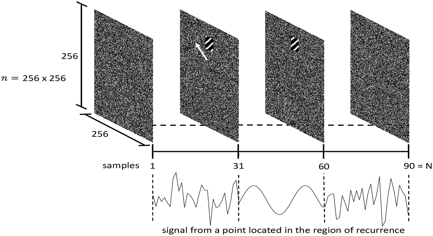
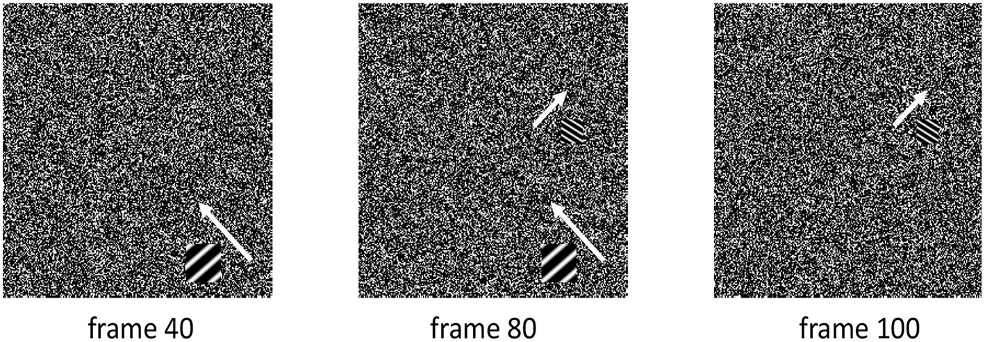
Figure 2. Example of spatio-temporally localized recurrence. A 2D sinusoidal wave of limited time duration appears in a specific region of a random noise image, and propagates in the direction indicated by the white arrow. The sequence consists of N = 90 frames, with the sine wave appearing at frame 31 and lasting for 30 frames until frame 60. The frame size is 256 × 256 points, while the region of recurrence has size 32 × 32. At the bottom, the signal associated with a point (a pixel) in the region of recurrence is depicted (90 sample long signal), showing the alternation between random noise and the sine wave. The matrix B corresponding to this case has a size of 65536 × 90.

3.1.1. Identification of the Most Relevant Points in the Geometric Structure—Spatial Detection of Recurrence

The first step is to identify the most relevant points in the geometric structure associated with a specific recurrent pattern. This is achieved by first generating a matrix B = (n × N), which collects the signals from all points in the structure (n points and N samples). Matrix B is then decomposed by means of PCA, using Singular Value Decomposition (SVD), such that B = USV^T, with U = (n × n) and V = (N × N) being orthogonal matrices collecting the left and right singular vectors, respectively, and S = (n × N) a rectangular diagonal matrix collecting the singular values of B on its diagonal. The rationale for using SVD is due to the assumption that spatio-temporal repetitive quasi-periodic patterns are expected to be associated with highly correlated signals at different points of the structure. This provides the ideal setting for PCA to describe this redundancy, which is expected to be picked-up by the first Principal Components (PCs) of B. At the same time this filters out possible uncorrelated information or noise from other points. Moreover, the output V of the SVD is independent of any permutation of the rows of B, making this step of the analysis independent of the specific geometric relationships among the points.

The second step is to identify how many PCs of B are required to properly determine a recurrent pattern in the structure. The full PC decomposition of B can be obtained as B = AZ, where $Z=\sqrt{N}{V}^T$ is the matrix collecting the PCs of B in its rows, and $A=\frac{1}{\sqrt{N}}US$ is the linear transformation connecting the PCs to the original variables. The most relevant PCs associated with a recurrent pattern are then found by looking at the normalized power spectrum P_j(f):

$\begin{array}{lll}{P}_j(f)& =\frac{|{\widehat{Z}}_j(f){|}^2}{{\displaystyle \underset{f}{max}}|{\widehat{Z}}_j(f){|}^2}& (2)\end{array}$

$\begin{array}{lll}\text{w}\text{h}\text{e}\text{r}\text{e}{\widehat{Z}}_j(f)& ={\displaystyle \sum _{\ell =0}^{N-1}}{Z}_j(\ell )e^{\frac{-2\pi i\ell f}{N}}& (3)\end{array}$

of each PC Z_j (with f being the frequency index), and by measuring the spectral concentration (SC) around the index ${\tilde{f}}_j$ of the dominant frequency peak in P_j(f) [14]. The spectral concentration is computed as:

$\begin{array}{ll}\text{S}{\text{C}}_j=\frac{{\displaystyle {\sum }_{f={\tilde{f}}_j-\frac{w_j}{2}}^{{\tilde{f}}_j+\frac{w_j}{2}}}{P}_j(f)}{{\displaystyle {\sum }_{f=0}^{N-1}}{P}_j(f)},& (4)\end{array}$

where w is the half height bandwidth of the frequency of the dominant peak at ${\tilde{f}}_j$. The rationale to look at the SC for selecting the most relevant PCs is that recurrence associated with repetitive (quasi-periodic and oscillating) patterns should show clear peaks in the power spectrum of the corresponding PCs. The most relevant PCs are identified as those whose SC is larger than a pre-defined threshold Γ (which is assumed to be dependent on the specific application). Figure 3 shows the power spectrum of the first PC of the recurrent pattern in Figure 2, together with the frequency index ${\tilde{f}}_j$ of the dominant peak and its half height bandwidth w_j for the computation of the SC of component Z_j.

FIGURE 3

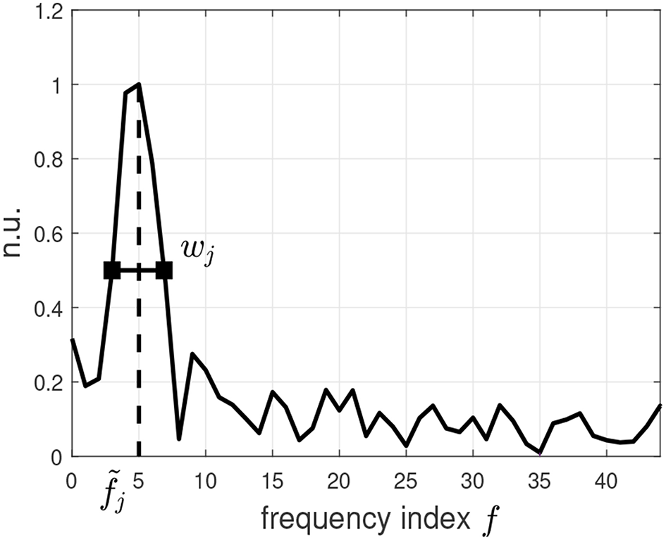
Figure 3. Normalized power spectrum of the first principal component of the matrix B from the example of Figure 2. The location of the index ${\tilde{f}}_j$ of the dominant frequency peak and its half height bandwidth w_j are also shown. The horizontal axis shows the frequency indices; the vertical axis shows the normalized power spectrum (n.u.: normalized units).

Once all relevant PCs of a recurrent pattern have been selected, the third step is to identify all points in the original geometric structure associated with those PCs, i.e., the points on which the selected PCs are reflected the most. This is achieved as follows: for each selected PC Z_j, the entries in the (n × 1) vector a_j, the j-th column of A, provide information about the contribution of Z_j to each point in the original structure. The most relevant points in the geometric structure associated with Z_j can therefore be defined as those points with the largest contribution from Z_j. The following criterion is used on a_j to select all relevant points associated with a selected Z_j. Given each entry a_j(i) of a_j, the vector ${\tilde{\text{a}}}_j$ is generated by taking the absolute value of each entry of a_j: ã_j(i) = |a_j(i)|, for i = 1, …, n. Then, for each entry ã_j(i) in ${\tilde{\text{a}}}_j$, location i is selected as relevant if ${ã}_j(i)>3{\sigma }_{{\tilde{\text{a}}}_j}$, where ${\sigma }_{{\tilde{\text{a}}}_j}$ denotes the standard deviation of the entries in ${\tilde{\text{a}}}_j$. Assuming that recurrence patterns are only present on limited regions of a structure, and for limited time, most of the points at each time instant are expected to be uncorrelated with those recurrence patterns, and they represent a sort of reference range. The multiplicand 3 is used to identify all points outside of this reference range. Figure 4-left shows the locations of the most relevant points associated with the recurrent pattern in Figure 2. Observe that the region of recurrence is identified properly, but several spurious points outside of this regions have been selected as well. To accurately identify regions associated with recurrent patterns, and filter out spurious points, the geometric information about proximity between the most relevant points is then taken into account in order to cluster neighboring relevant points together. This can be achieved in a similar way to finding connected nodes in a undirected graph, and any suitable technique for this task can be employed. An (application dependent) threshold can then be applied to define the minimum size (number of points) that a cluster should have to be considered a region of recurrence, and to filter out all small clusters composed by spurious points. Figure 4-right shows the result of applying the geometric information to the relevant points in Figure 4-left, in order to identify the recurrent regions in a structure.

FIGURE 4

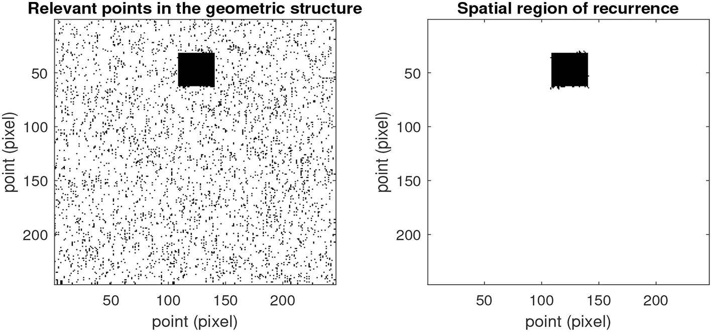
Figure 4. (Left) locations of the most relevant points associated with the recurrent pattern in Figure 2. (Right) region of recurrence identified after applying the geometric information to all relevant points identified, and a threshold on the minimum number of points a region of recurrence should contain (set to 100 points for this example).

3.1.2. Spatio-Temporal Detection of Recurrence

To be able to estimate the time span of a region of recurrence in a geometric structure, the multi-variate signal can be split up into (overlapping) time windows, and the algorithm for spatial detection of recurrence introduced in the previous section can be applied to each window individually. All clusters identified in a window need then to be compared with those found in the previous window, to be able to say for each cluster whether it is a new cluster or not, or whether a cluster from the previous window has ceased. Experience shows that the window size p and the overlap between windows q, are application dependent, as it is to be expected. Figure 5 shows the result of applying the proposed approach for spatio-temporal detection of recurrence to the case of Figure 2, involving a time limited 2D sinusoidal wave appearing at a specific location in a sequence of random noise images.

FIGURE 5

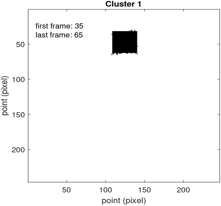
Figure 5. Example of application of the framework for spatio-temporal detection of recurrence introduced in section 3.1 to the example of Figure 2. Shown is a summary of the analysis as outputted by our software. In black the detected recurrence area is indicated. The estimated time interval (frame range) of the recurrent pattern is also shown.

For the estimate of the time interval of a region of recurrence, we used the first and last window where the region was detected. The mid points of those windows are used to estimate the start and the end of the time interval of recurrence, respectively. In the example, the estimated interval (from frame 35 to 65, as displayed in Figure 5) is close to the actual time interval of the recurrent pattern (from frame 31 to 60). The result shown in Figure 5 was obtained with a window size p = 30 frames, and an overlap q = 20.

3.2. Multi-Variate Recurrence Plots

As mentioned before, RPs provide a way to visualize and quantify recurrent behavior of the phase-space trajectory of a dynamical system [2]. According to Takens' theorem the dynamics of a uni-variate process x(k) can be represented in phase space using an appropriate time-delay embedding, producing the embedded vector:

$\begin{array}{ll}\text{x}(k)={(x(k),x(k+\tau ),\dots ,x(k+\tau (m-1)))}^T& (5)\end{array}$

with time-delay τ and embedding dimension m, providing a vector of size m × 1. Recurrence R_ij between two points x(i) and x(j) in the phase-space is measured by computing the distance between those two points. Traditionally, the Euclidean distance is used to compute the proximity of two points in the phase space.

Given a multi-variate process, the uni-variate framework in (5) needs to be extended to handle multi-variate (spatio-temporal) data. This would allow to process the signals from all points of a recurrent region simultaneously, and take into account the contribution of space and time together. A multi-variate RP can be generated as follows: the matrix X of size ℓ × M is defined, which collects the set S of points constituting a recurrent region (ℓ = |S| ≤ n), and all samples in the set T that constitutes the time span of the recurrence in that region (M = |T| ≤ N). The rows of X can be viewed as a multi-variate time series x_i(k), i = 1, …, ℓ and k = 1, …, M, which denotes the i-th signal sampled at discrete time k. The dynamics of a process x_i(k) can be then reconstructed by considering delayed copies of each of the signals forming the delay vectors:

$\begin{array}{l}x(k)=(x_1(k),x_1(k+{\tau }_1),\dots ,x_1(k+(m_1-1){\tau }_1),\dots ,\\ x_{\ell }(k),x_{\ell }(k+{\tau }_{\ell }),\dots ,x_{\ell }(k+(m_{\ell }-1){\tau }_{\ell }){)}^T.\end{array}$

As in the multi-variate case of a dynamical system, the embedding dimension of all ℓ signals can be fixed to m_i = 1, i = 1, …, ℓ, thus giving the phase space representation x(k) = (x₁(k), x₂(k), …, x_ℓ(k)), as proposed in Nichols et al. [8]. Each column of X is then assumed to provide an “embedded” vector x(k). This formulation allows to investigate the temporal recurrence over the entire surface covered by a recurrent region. An unthresholded RP can then be generated by measuring the distance between each column x(k), and every other column in X.

As a distance measure, we propose to use the cosine of the angle between two vectors instead of the Euclidean distance, namely:

$\begin{array}{ll}d(\text{x}(i),\text{x}(j))=\frac{\text{x}{(i)}^T\text{x}(j)}{\left|\right|\text{x}(i)\left|{|}_2\right|\left|\text{x}(j)\right|{|}_2}& (6)\end{array}$

The rationale for this choice is that this distance provides a normalized correlation which is not affected by the magnitude of the vectors (for two signals, that means that the shapes of the signals are compared without being influenced by their respective amplitudes). This approach for generating a multi-variate RP was used in Meste et al. [15] to investigate temporal recurrence of spatial patterns of the electrical activity of the heart, as recorded on the body surface, in patients affected by AF (for which several electrical signals were recorded on the body surface). This helped improving both noninvasive characterization of the progression of the disease and outcome prediction of a specific therapy.

Figure 6 shows an example of a multi-variate RP for the case presented in Figure 2. Figure 6 top-left shows the multi-variate RP computed on all points and all samples (X = B of size n × N). It can be noticed how the RP is dominated by the random noise in the system (only the main diagonal stands out, which is related to the autocorrelation at lag zero), while the recurrent patterns associated with the 2D sinusoidal wave is completely concealed by the noise of the system. On the other hand, when a multi-variate RP is generated using only the relevant points in the geometric structure, the recurrent patterns associated with the 2D sinusoidal wave stand above the random noise (X = B_{i∈S; 1:N} of size ℓ × N). This is shown in Figure 6 top-right, from which the temporal extension of the recurrent pattern can be clearly deduced from the RP (lasting from sample 31 to sample 60). Figure 6 bottom-left shows the result of generating a multi-variate RP using only the points within the region of recurrence, and the time interval corresponding to the temporal extension of the recurrent pattern (X = B_{i∈S; j∈T} of size ℓ × M; from frame 31 to frame 60). Finally, Figure 6 bottom-right shows the multi-variate RP computed on the region of interest and time interval reported in Figure 5, identified by the spatio-temporal approach proposed in section 3.1.

FIGURE 6

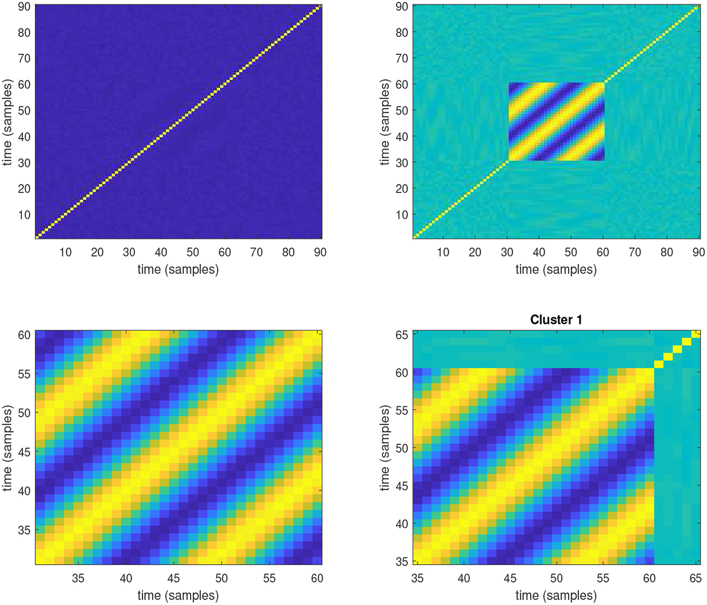
Figure 6. Multi-variate RP for the case presented in Figure 2. (Top-left) The multi-variate RP computed on all points and all samples (X = B of size n × N). (Top-right) Multi-variate RP is generated using only the relevant points in the geometric structure (set S). (Bottom-left) Multi-variate RP using only the points within the region of recurrence (set S), and the time interval corresponding to the temporal extension of the recurrent pattern (T = {31, …60}), i.e., frame 31 through 60. (Bottom-right) Multi-variate RP computed on the region of interest and time interval (frame 35 through 65) reported in Figure 5.

4. Simulations

Two numerical simulations are presented in this section. The first one shows the ability of the proposed approach to handle multiple recurrent patterns simultaneously occurring in a geometric structure. The second one shows the ability of the proposed approach to detect recurrent patterns from spiraling waves, which may occur in several real world problems, among which cardiac arrhythmia like AF. All analysis and computations were performed in MATLAB (MATLAB and Statistics Toolbox Release 2018a, The MathWorks, Inc., Natick, MA, USA). Code can be requested from the authors.

4.1. 2D Sine Waves

The first simulation concerns a sequence of random noise images (each frame of size 256 × 256 points), with two different 2D sinusoidal waves of limited time duration appearing in two different regions of the random images. The sequence is composed of N = 150 frames, with the first sinusoidal wave starting at frame 40 and lasting for 60 frames (region of recurrence of size 32 × 32 points; Figure 7-left), and the second sinusoidal wave starting at frame 80 and lasting for 60 frames (region of recurrence of size 20 × 20 points; Figure 7-right). The two sinusoidal waves are therefore simultaneously present in twenty frames (Figure 7-middle), while having different directions of propagation (indicated by the white arrows in Figure 7), different frequencies, and different speeds of propagation (with the smaller wave having a higher speed than the larger wave). The two waves were generated from Equation (1), with the following settings, first sine wave: f = 1/12, $\theta =\frac{2\pi }{7}$, $\varphi (t)=\frac{\pi }{9}t$, for t = 0, 1, 2, …; second sine wave: f = 1/5, $\theta =\frac{2\pi }{3}$, and $\varphi (t)=\frac{\pi }{9}t$, for t = 0, 1, 2, ….

FIGURE 7

Figure 7. Simulation characterized by a sequence of random images with two different 2D sinusoidal waves of limited time duration, appearing in two different regions of the random images. The two sinusoidal waves are simultaneously present over 20 frames, and they have different direction of propagation (indicated by the white arrows), different frequency, and different speed of propagation (with the smaller wave having a higher speed than the larger wave).

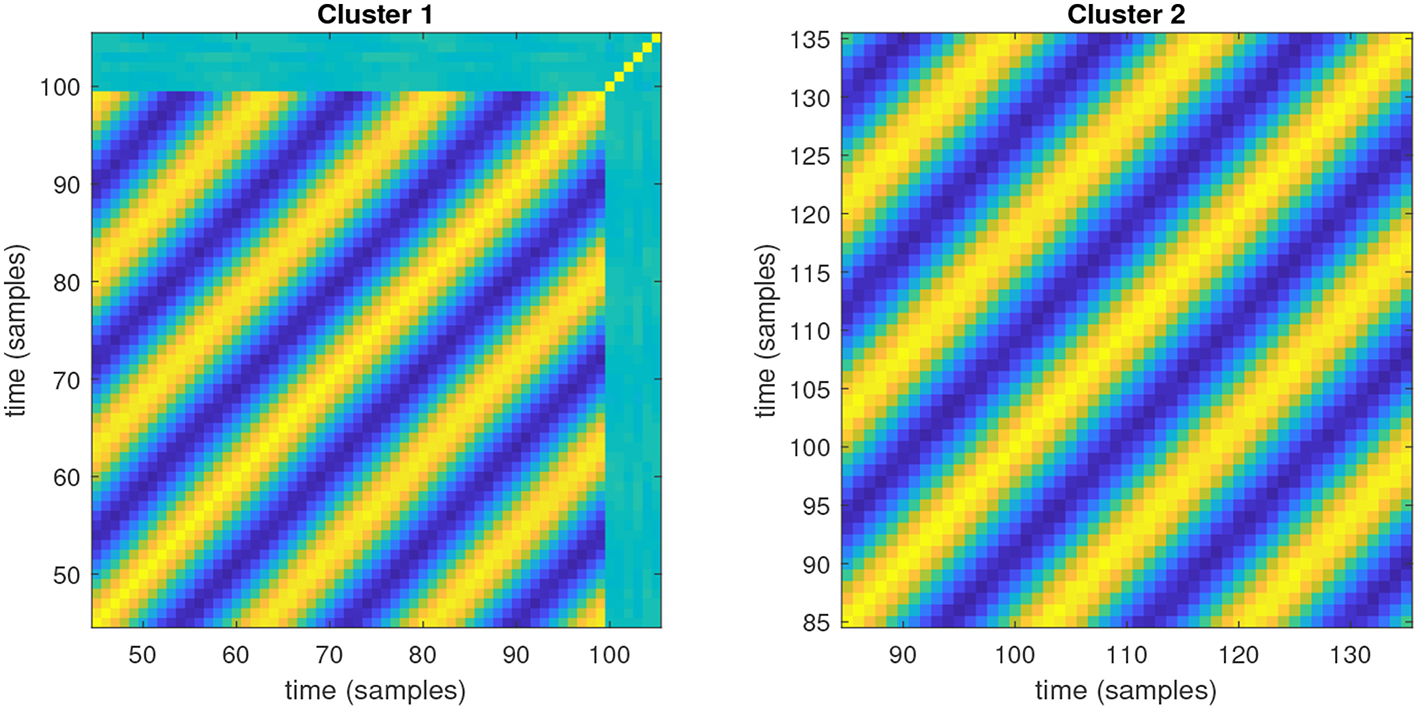
Figure 8 shows the result of applying the framework proposed in section 3.1 for spatio-temporal detection of recurrence to this example. For this, the following settings were used: a window size p = 30 samples, with overlap q = 20 samples, a threshold Γ = 0.25 for the spectral concentration, and a minimum size of 100 points for a cluster to be considered a valid region of recurrence. From Figure 8, it can be noticed how the proposed framework accurately detects both the locations of the two regions of recurrence (also avoiding generation of spurious regions), and their corresponding time supports (cluster 1: actual time interval from 40 to 99, estimated from 45 to 105; cluster 2: actual time interval from 80 to 139, estimated from 85 to 135).

FIGURE 8

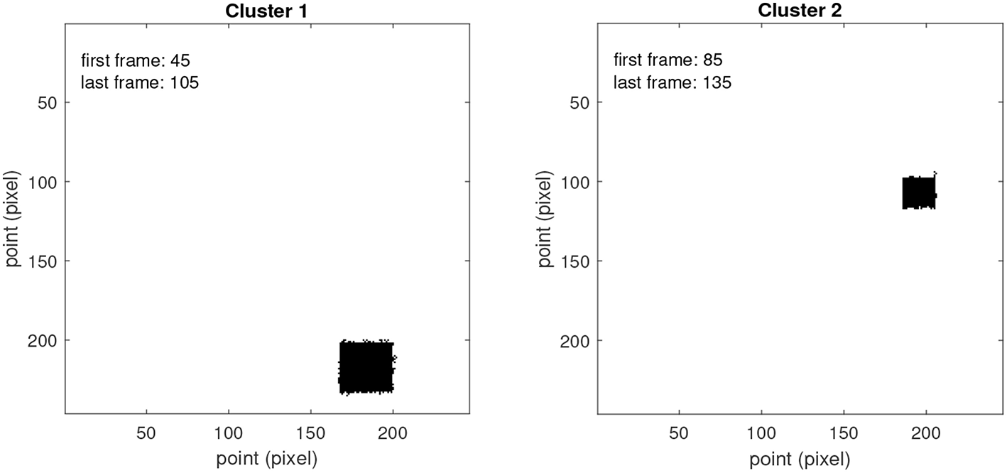
Figure 8. Result of applying the framework for spatio-temporal detection of recurrence introduced in section 3.1 to the example of Figure 7. The estimated time intervals of the recurrent patterns are also shown.

Figure 9 shows the multi-variate RPs of the two recurrent regions depicted in Figure 8, computed over the time intervals estimated for the corresponding clusters.

FIGURE 9

Figure 9. Multi-variate RPs computed on the regions of interest and time intervals reported in Figure 8.

4.2. 2D Periodic Spiraling Wave

The second simulation concerns a sequence of random noise images (each frame with a size of 300 × 300 points). The sequence is composed of N = 130 frames, with a 2D periodic spiraling wave appearing at frame 21, and lasting for 80 frames (with a period of approximately 25 frames; the region of recurrence is of size 128 × 128 points; Figure 10 shows two periods of the spiraling wave). The spiraling pattern was simulated using the complex Ginzburg-Landau equation in 2D (by means of pseudo-spectral code and exponential time differencing, as described in Cox and Matthews [16]). The complex Ginzburg-Landau equation has been used to describe several physical phenomena, among which nonlinear waves, superconductivity, and strings in field theory [17]. The equation is given by:

${\partial }_{t}A=A+(1+ib)\Delta A-(1+ic)|A{|}^{2}A,$

where A is a complex function of (scaled) time t and (two dimensional) space, and the real parameters b and c characterize linear and nonlinear dispersion. The simulation in Figure 10 was generated by setting b = 0 and c = 1.2. The complex Ginzburg-Landau equation allows to simulate spiral turbulence in two dimensions, which can be regarded as a model of AF. Indeed, cardiac arrhythmia such as AF are characterized by spatially complex dynamics generated as multiple excitation waves that propagate through the cardiac tissue, merging and breaking up [18]. Unlike the previous simulation, this simulation offers therefore a more realistic example of a spatially complex periodic pattern, and it provides a test bench for the application of the proposed framework for spatio-temporal detection of recurrence to the characterization of atrial activity propagation patterns during AF, which is discussed in section 5.

FIGURE 10

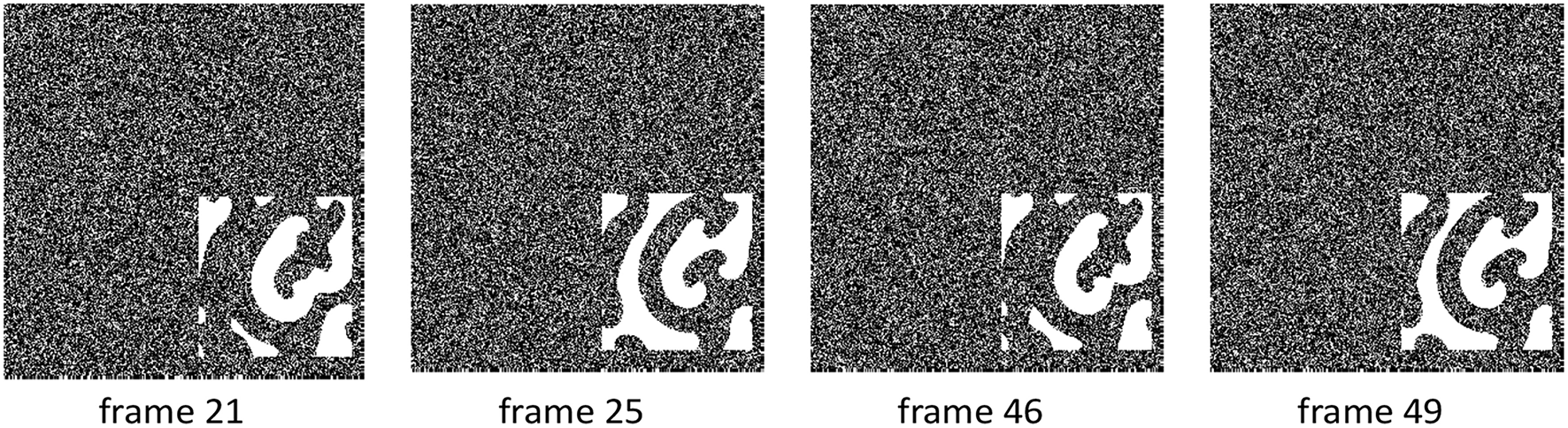
Figure 10. Simulation characterized by a sequence of random images with a spiraling wave of limited time duration added to it. The spiraling pattern was obtained by means of a complex Ginzburg-Landau equation, with parameters b = 0 and c = 1.2. The simulation shows two periods of the spiraling wave.

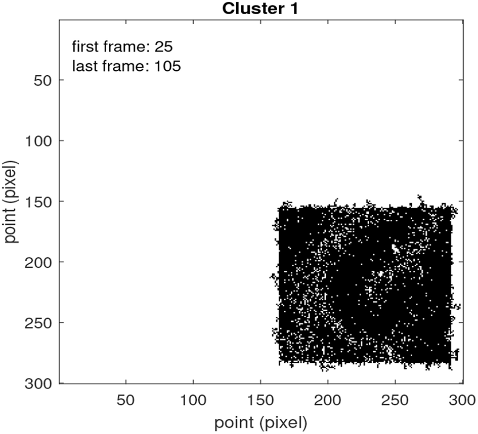
Figure 11 shows the result of applying the spatio-temporal detection of recurrence to this example. For this, the following settings were used: a window p = 40, with overlap q = 30, a threshold Γ = 0.25 for the spectral concentration, and a minimum size of 100 points for a cluster to be considered a valid region of recurrence. From Figure 10, it can be noticed how the proposed framework admits accurate detection of the location of the region of recurrence, and of its corresponding time interval (actual time interval from 21 to 101, estimated from 25 to 105). A longer window size was required for this simulation to be able to detect recurrence of the spiraling wave. This was likely due to the fact that the spiral wave is sparser both in space and time.

FIGURE 11

Figure 11. Result of applying the framework for spatio-temporal detection of recurrence introduced in section 3.1 to the example of Figure 10. The estimated time interval of the recurrent pattern is also shown.

Figure 12 shows the multi-variate RP of the recurrent region depicted in Figure 10, computed over the time interval estimated for the corresponding cluster.

FIGURE 12

Figure 12. Multi-variate RP computed on the region of interest and time interval reported in Figure 11.

5. Application to Atrial Fibrillation

5.1. Experimental Setup

The animal study performed to acquire the data used in this study was carried out in accordance with the principles of the Basel Declaration and regulations of European directive 2010/63/EU. The local ethical board for animal experimentation of Maastricht University approved the protocol. Epicardial (outer surface of the heart) high-density direct contact mapping was performed in an ovine model of acute atrial fibrillation (AF). Uni-polar electrograms were measured on the left atrial free wall during an open-thorax procedure with a regular grid of electrodes (16x16 electrodes, 1.5mm inter-electrode distance, 1 KHz sampling frequency, see Figure 13A). In a healthy adult sheep, acetylcholine was delivered intracoronary, which shortened the effective refractory period of the atrial action potential, thereby shortening the AF cycle length and stabilizing AF. Infusion rate was adjusted to reach a sufficiently short AF cycle length at which more complex patterns of AF (i.e., multiple wave fronts per cycle) could be observed.

FIGURE 13

Figure 13. Application of the spatio-temporal recurrence detection framework to high-density contact mapping recordings in an ovine model of AF. (A) a high-density grid of electrodes was used to record conduction patterns during AF in a healthy adult sheep, on the left atrial free wall during an open-thorax procedure. (B) a recurrence plot of a 10 s recording based on activation-phase similarity. Overall recurrence is limited and short-lasting (recurrence rate: 0.23% determinism: 88.17%, minimal diagonal line length 1 AF cycle). (C) application of the spatio-temporal recurrence detection framework produced a heat map of electrode-cluster incidence (left) and corresponding candidate recurrence regions (right). (D) Recurrence plots of the selected regions with corresponding colors (blue and red), with increased recurrence [recurrence rates: 5.31% (blue) and 1.55% (red), determinism: 83.79% (blue), and 56.18% (red)].

5.2. Recurrence Analysis

Recurrence of wave patterns was determined in a selected segment of the mapping, which comprised 10 s of AF, with an average cycle length of 67 ms (~15 Hz). Recurrence analysis was based on automated annotation of local atrial deflections and activation-based phase map similarity as described in previous work [6, 19]. In short, an activation guided phase signal was computed for each signal, setting the moment of phase inversion equal to the local activation time. The linear phase (−π to π) was interpolated for every interval between activations. Based on these phase signals, phase maps were constructed for all time steps. The distance between two phase maps was calculated as the average absolute phase difference over all electrodes. This was executed for every possible comparison between time steps within the 10 s recording. Recurrent patterns were defined as phase maps with a distance $<\frac{\pi }{4}$, corresponding to $\frac{1}{8}$ of the AF cycle length.

5.3. Application of the Framework for Spatio-Temporal Detection of Recurrence

The proposed framework for spatio-temporal detection of recurrence was applied to the uni-polar electrograms. The frequency content around the fundamental frequency of AF was emphasized by filtering the electrograms with a band-pass filter (40–250 Hz, 3rd order, zero-phase Chebyshev), followed by rectification and a low-pass filter (20 Hz, 3rd order, zero-phase Chebyshev). Window size was set to p = 10 AF cycles (~670 ms) with a 50% overlap (q = 5 AF cycles), a threshold Γ = 0.25 for spectral concentration, and a minimum size of 20 electrodes for a cluster. Deviating slightly from the approach used in the simulations, the identification of regions eligible for recurrence analysis was performed by creating a heat map of the number of times each electrode was selected as part of a cluster in each window. Regions were identified as clusters of electrodes that were selected in at least 75% of the windows. The rationale behind this procedure is that in the context of AF, the interest is in finding regions that harbor both recurrent and frequent patterns that may act as local drivers that maintain AF. This procedure also accounts for potential minor drifting of the dominant recurring patterns.

Figure 13 shows the results of the case study in the ovine model of AF. The RP for the whole mapping area (Figure 13B) shows that overall recurrence rate is very limited, which indicates that there are almost no wave front patterns that re-occur. Close to the diagonal there are a few, short-lived recurrences that however do not reappear later on. Applying spatio-temporal recurrence detection, a heat map of electrode-cluster incidence was determined that shows two distinct regions of frequently selected electrodes (Figure 13C). RPs for these two regions are shown in Figure 13D, in blue and red. Clearly, these two regions - most notably the larger region in blue - have an increased recurrence rate compared to the RP of the full mapping area. This shows the benefit of using the suggested framework to unveil regions of recurrence in spatio-temporal data from a complex dynamical system, which would be otherwise concealed by using all the spatio-temporal information available.

6. Discussion

This study proposed a novel framework for spatio-temporal detection of recurrence in complex dynamical systems characterized by repetitive (quasi-periodic) spatio-temporal patterns. This framework allows to address the following questions: whether a recurrent pattern is present in the geometric structure, where it is located (in which region of the geometric structure), and when it occurs (at what time instants it appears and then disappears). This is relevant since several dynamical systems are characterized by a well defined spatial organization, and accurate localization of recurrence both in space and time becomes important to be able to properly describe the recurrent behavior of such systems, and filter out any noise or unwanted information. This can be seen in Figure 6, which displays the multi-variate RP of a simple example, a 2D sinusoidal wave traveling in a limited region of a noisy image. When all spatial and temporal information is considered, the dynamic behavior associated with the sinusoidal wave is concealed by the noise, and the typical RP of white noise is obtained. On the other hand, the typical RP of a sinusoidal wave is properly retrieved when only the spatio-temporal information associated with the region of recurrence is used.

The two numerical simulations presented in section 4 suggest that the proposed framework is able to achieve a detailed identification of the spatial and temporal locations of different types of spatio-temporal repetitive patterns in a dynamical system. The first simulation shows that an accurate identification in both space and time is possible even when several recurrent patterns are simultaneously present in the geometric structure of a dynamical system. The second simulation shows that accuracy is also maintained with more complicated types of recurrent patterns like spiral waves from reaction diffusion models, simulated by means of the complex Ginzburg-Landau equation, whose recurrent patterns become sparser both in space and time, and thus more difficult to be detected. This scenario is also encountered in cardiac arrhythmia like AF, in which abnormal electrical activity may generate and propagate in specific regions of the atrial tissue, which may also offer the physiological conditions for this activity to self-perpetuate over a certain time span. When applied to actual invasive recordings of atrial activity during AF in an animal model, the proposed framework was able to unveil regions on the atrial walls characterized by recurrent behaviors, which were not visible from the RP generated from the full available spatio-temporal data. This is relevant, as an accurate spatial and temporal identification of those regions may help characterize the progression of the disease, the level of impairment of the cardiac tissue, and improve patients stratification and personalize therapy [20].

The proposed framework was also tested on simulations similar to those of Figures 2, 7, but with the background noise replaced by a 2D sinusoidal wave covering all the geometric structure and lasting for the entire duration of the simulation (results not presented in this study). This was done in order to test the ability of the framework to detect regions of spatio-temporal repetitive patterns in presence of a background global repetitive pattern. The preliminary results of this analysis showed that the framework could correctly detect the regions of recurrence and separate those from the background activity. In turn, this suggests that the method should be able to handle the contemporary presence of different temporal structures in different areas and at different time/spatial scales, and to identify meaningful temporal structures with low percentage of variance explained. However, this should be thoroughly addressed in a future study. In this respect, Giuliani et al. [21] showed that addition of artificial noise to a multi-variate dataset before PCA improved the discrimination between weak periodic signals and noise inherent in the data. In a similar way, Poon and Barahona [22] proposed the controlled addition of white or colored noise to short and noisy time series data to track the onset of deterministic chaos and to give a relative measure of chaos intensity. The framework introduced in this study may benefit from such a controlled addition of noise to the spatio-temporal data to improve discrimination of different temporal structures simultaneously present in different areas and at different time/spatial scales. Similarly, Zbilut et al. [23] used cross-recurrence to extract periodic signals up to very low signal-to-noise ratio. It would be worthwhile to investigate whether replacing matrix B in the current framework with the covariance matrix of the multi-variate time series data may improve identification of the significant points in the geometric structure, and reduce spurious points due to noise.

Several extensions of RP techniques for spatially distributed data have been introduced. In this respect, Riedl et al. [12] proposed multi-scale recurrence analysis of spatio-temporal data as a way to take spatial patterns of different scales and with different rhythms into account. They showed that this approach is able to both separate mixed regular patterns of specific scales and rhythms and also to reveal large-scale rhythms beyond the dominant small-scale dynamics in spatial distributed systems. The framework proposed in this study could be integrated with this and other multi-variate RP approaches, in order to improve multi-variate RQA of spatio-temporal data.

The task of detecting the start and end points of a recurrent pattern may appear very similar to the one of change point detection (CPD) in time series data [24]. CPD is about identifying the time point(s) in a time series such that observations follow a certain statistical distribution up to that point and a different distribution after that point [25]. In this respect, Hu et al. [26] recently proposed the use of RPs to improve CPD in multi-variate time series data. However, the sudden appearance of a spatio-temporal repetitive pattern in a multi-variate time series represents a very specific type of change, which may not be reflected in a statistical difference in the distributions of the observations before and after the change. In a future study, it may be worthwhile to investigate whether an RP-based CPD approach could be used as an alternative to the sliding window approach suggested in this study, in order to improve the accuracy in the estimation of the time interval of a recurrent patter, after the most significant points in the geometric structure have been identified.

In this study, we did not analyze the influence of the noise level on the accuracy in the detection of spatio-temporal recurrence, which should be addressed by a future study. One limitation of the proposed framework is that it only considers information about proximity when clustering neighboring points to build a region of recurrence. Additional information could be taken into account, such as distances between the points, which may become relevant when clustering points in arbitrary irregular geometric structures.

7. Conclusion

In this study, we presented a novel framework for spatio-temporal detection of recurrence in complex dynamical systems characterized by a well defined spatial structure. This framework focuses on spatio-temporally localized repetitive patterns and is able to retrieve the correct recurrence plots associated with known traveling waves in a geometric structure, by focusing on the spatial regions and time intervals involved by a recurrence behavior, and leaving out all unwanted information. This framework may be integrated with state of the art methods for multi-scale and multi-variate recurrence plots, to help improve recurrence quantification analysis of spatio-temporal data.

Data Availability

The datasets generated for this study are available on request to the corresponding author.

Ethics Statement

The animal study was reviewed and approved by Animal Ethics Committee Maastricht University Secretariat DEC, UNS 50, box 48 6200MD Maastricht, The Netherlands.

Author Contributions

PB, RP, OM, and JK developed the theoretical formalism. PB designed the numerical experiments and analyzed the data. SZ and AvH designed and performed the animal experiments, and analyzed the corresponding data. PB wrote the first draft of the manuscript. All authors contributed to the final version and contributed in interpreting the results.

Conflict of Interest Statement

The authors declare that the research was conducted in the absence of any commercial or financial relationships that could be construed as a potential conflict of interest.

References

1. Marwan N, Kurths J, Saparin P. Generalised recurrence plot analysis for spatial data. Phys Lett A. (2007) 360:545–51. doi: 10.1016/j.physleta.2006.08.058

CrossRef Full Text | Google Scholar

2. Eckmann JP, Oliffson Kamphorst S, Ruelle D. Recurrence plots of dynamical systems. Europhys Lett. (1987) 4:973–77.

Google Scholar

3. Sipers A, Borm P, Peeters R. On the unique reconstruction of a signal from its unthresholded recurrence plot. Phys Lett A. (2011) 375:2309–21. doi: 10.1016/j.physleta.2011.04.040

CrossRef Full Text | Google Scholar

4. Sipers A, Borm P, Peeters R. Robust reconstruction of a signal from its unthresholded recurrence plot subject to disturbances. Phys Lett A. (2017) 381:604–15. doi: 10.1016/j.physleta.2016.12.028

CrossRef Full Text | Google Scholar

5. Zbilut JP, Webber CL. Embeddings and delays as derived from quantification of recurrence plots. Phys Lett A. (1992) 171:199–203.

Google Scholar

6. Van Hunnik A, Zeemering S, Podziemski P, Simons J, Gatta G, Hannink L, et al. Stationary atrial fibrillation properties in the goat do not entail stable or recurrent conduction patterns. Front Physiol. (2018) 9:947. doi: 10.3389/fphys.2018.00947

PubMed Abstract | CrossRef Full Text | Google Scholar

7. Romano MC, Thiel M, Kurths J, von Bloh W. Multivariate recurrence plots. Phys Lett A. (2004) 330:214–23. doi: 10.1016/j.physleta.2004.07.066

CrossRef Full Text | Google Scholar

8. Nichols JM, Trickey ST, Seaver M. Damage detection using multivariate recurrence quantification analysis. Mech Syst Signal Process. (2006) 20:421–37. doi: 10.1016/j.ymssp.2004.08.007

CrossRef Full Text | Google Scholar

9. Vasconcelos D, Lopes SR, Viana RL, Kurths J. Spatial recurrence plots. Phys Rev E. (2006) 73:056207. doi: 10.1103/PhysRevE.73.056207

PubMed Abstract | CrossRef Full Text | Google Scholar

10. Marwan N, Romano MC, Thiel M, Kurths J. Recurrence plots for the analysis of complex systems. Phys Rep. (2007) 438:237–329. doi: 10.1016/j.physrep.2006.11.001

CrossRef Full Text | Google Scholar

11. Prado TL, Galuzio PP, Lopes SR, Viana RL. Spatial recurrence analysis: a sensitive and fast detection tool in digital mammography. Chaos. (2014) 24:013106. doi: 10.1063/1.4861895

PubMed Abstract | CrossRef Full Text | Google Scholar

12. Riedl M, Marwan N, Kurths J. Multiscale recurrence analysis of spatio-temporal data. Chaos. (2015) 25:123111. doi: 10.1063/1.4937164

PubMed Abstract | CrossRef Full Text | Google Scholar

13. Chen CB, Yang H, Kumara S. Recurrence network modeling and analysis of spatial data. Chaos. (2018) 28:085714. doi: 10.1063/1.5024917

PubMed Abstract | CrossRef Full Text | Google Scholar

14. Castells F, Rieta JJ, Millet J, Zarzoso V. Spatiotemporal blind source separation approach to atrial activity estimation in atrial tachyarrhythmias. IEEE Trans Biomed Eng. (2005) 52:258–67. doi: 10.1109/TBME.2004.840473

PubMed Abstract | CrossRef Full Text | Google Scholar

15. Meste O, Zeemering S, Karel J, Lankveld T, Schotten U, Crijns H, et al. Noninvasive recurrence quantification analysis predicts atrial fibrillation recurrence in persistent patients undergoing electrical cardioversion. Proc Comput Cardiol. (2016) 43:677–80. doi: 10.22489/CinC.2016.199-342

CrossRef Full Text | Google Scholar

16. Cox SM, Matthews PC. Exponential time differencing for stiff systems. J Comput Phys. (2002) 176:430–55. doi: 10.1006/jcph.2002.6995

CrossRef Full Text | Google Scholar

17. Aranson IS, Kramer L. The world of the complex Ginzburg-Landau equation. Rev Modern Phys. (2002) 74:99–143. doi: 10.1103/RevModPhys.74.99

CrossRef Full Text | Google Scholar

18. Byrne G, Marcotte CD, Grigoriev RO. Exact coherent structures and chaotic dynamics in a model of cardiac tissue. Chaos. (2015) 25:033108. doi: 10.1063/1.4915143

PubMed Abstract | CrossRef Full Text | Google Scholar

19. Zeemering S, Bonizzi P, Maesen B, Peeters R, Schotten U. Recurrence quantification analysis applied to spatiotemporal pattern analysis in high-density mapping of human atrial fibrillation. In: 2015 37th Annual International Conference of the IEEE Engineering in Medicine and Biology Society (EMBC) (Milan). (2015). p. 7704–7. doi: 10.1109/EMBC.2015.7320177

PubMed Abstract | CrossRef Full Text | Google Scholar

20. Zeemering S, Lankveld TAR, Bonizzi P, Limantoro I, Bekkers SCAM, Crijns HJGM, et al. The electrocardiogram as a predictor of successful pharmacological cardioversion and progression of atrial fibrillation. EP Eur. (2017) 20:e96–104. doi: 10.1093/europace/eux234

PubMed Abstract | CrossRef Full Text | Google Scholar

21. Giuliani A, Colosimo A, Benigni R, Zbilut JP. On the constructive role of noise in spatial systems. Phys Lett A. (1998) 247:47–52.

Google Scholar

22. Poon CS, Barahona M. Titration of chaos with added noise. Proc Natl Acad Sci USA. (2001) 98:7107–12. doi: 10.1073/pnas.131173198

PubMed Abstract | CrossRef Full Text | Google Scholar

23. Zbilut JP, Giuliani A, Webber CL. Detecting deterministic signals in exceptionally noisy environments using cross-recurrence quantification. Phys Lett A. (1998) 246:122–8.

Google Scholar

24. Page ES. On problems in which a change in a parameter occurs at an unknown point. Biometrika. (1957) 44:248–52.

Google Scholar

25. Maboudou-Tchao EM, Hawkins DM. Detection of multiple change-points in multivariate data. J Appl Stat. (2013) 40:1979–95. doi: 10.1080/02664763.2013.800471

CrossRef Full Text | Google Scholar

26. Hu M, Zhou S, Wei J, Deng Y, Qu W. Change-point detection in multivariate time-series data by recurrence plot. WSEAS Transact Comput. (2014) 13:592–9.

Google Scholar