Non-Gaussian Penalized PARAFAC Analysis for fMRI Data

1. Introduction

ICA is one of the most popular methods to analyze fMRI single or group data especially when the time courses are not available [1–4], such as the application of autism experiments [5]. Unlike general linear model (GLM) [6], ICA is a more general and totally data-driven method to decompose the mixed data into mixing matrix and source signals. One fundamental prerequisite requirement of ICA is that the distributions of the independent source signals must be non-Gaussian [7]. So under this assumption, because Gaussian variable has the largest entropy among all random variables with equal variance, one popular algorithm called fastICA [7] decomposes the data by projecting the data onto the unmixing directions, such that the projected data have the maximum non-Gaussianity. Such unmixing directions of the inverse of the mixing matrix are mutual orthogonal and can be calculated by the Newton algorithm. The projected data form independent source signals. In the application of fMRI data (temporal × spatial), we usually call these source signals spatial components.

Many variants and improvements of ICA have developed in the past decade [8]. In the application of fMRI, the data usually have temporal-spatial information. We can use such information as the reference or constraint to improve the accuracy and robustness of the spatial components. The temporal information can be the time courses of design matrix in the experiment [9, 10]. The spatial information can be the atlas-defined masks [11, 12] or the cortex based information [13]. In some situation, the independent constraints are too strong to hold for some correlated spatial components. Subspace ICA [14–16] divides the spatial components into several groups and allows certain correlation of the components within the same groups. Multi-dimensional ICA [17] or topographic ICA [18] models the dependence through the spatial structure of the fMRI data, such as the neighboring voxels. Considering the sparsity character of the spatial components of the fMRI data, we can add the sparsity constraint to the fastICA to impose this character of the spatial components [19].

Besides the above developments of ICA to improve the accuracy and robustness of spatial components through the characters of themselves, it is very natural to consider the presence of the Gaussian noise in the fMRI data. The earlier work in Hyvärinen [20, 21] used a joint likelihood or the Gaussian moments to address this issue. Probabilistic ICA(PICA) [22] is another way to generalize the noise free ICA to incorporate the Gaussian noise. PICA assumes that the noise covariance is isotropic so that PICA could use a similar formula comparing with PPCA [23] to estimate and remove the noise before decomposing the data.

FMRI data usually contains multiple subjects as a group data. The heuristic way to process the group data is either combining the results of each subject or taking the average of all subjects. Beckmann and Smith [24] developed a three-mode ICA algorithm named tensorial probabilistic ICA (TPICA), which is suitable to decompose the group fMRI data into three modes: subject × temporal × spatial. Basically, as an extension of the PICA, TPICA not only decomposes fMRI data into the mixing matrix and spatial components by PICA, but also continues to decompose the mixing matrix to tensor product of time courses and subject loadings. In TPICA, the mode of spatial components has the priority to be processed, while the other two modes are estimated by one-rank approximations of mixed matrix. Based on TPICA, we can continue to refine the spatial components modeling by Gaussian mixture model and divide the tensor product of mixing matrix into different groups. This work has been completed in Guo [25] and Guo and Pagnoni [26]. The solution can be approximated by EM [27].

Parallel Factor Analysis (PARAFAC) is another popular method that processes three-mode data [28–30] and is becoming a new approach to process brain information and big data [31, 32]. Unlike TPICA, three modes are equally processed in PARAFAC. By the alternating least square (ALS) approach, one mode is estimated by least-squares from observed fMRI data while fixing other two modes. The three modes are iterated and alternated until the algorithm reaches convergence. PARAFAC does not require the independent constraint of the mode to achieve the solutions. One important property of PARAFAC is that the solution is unique under proper conditions [28]. However because PARAFAC highly relies on the effective decomposition of least-squares, it may converge to some degenerate solutions if one mode of the data can not meet the full rank requirement of the least-squares. Models with perfect collinearity are not estimable because there is an infinite number of solutions that could fit the data equally well. While in fMRI data, it is reasonable to find significant collinear relationships of the subject loadings mode within two similar subjects. In addition, PARAFAC also may converge very slowly solved via ALS [24] due to inaccurate estimation of the number of the spatial components. Based on these reasons and some experiments, the authors of TPICA [24] concluded that TPICA is more robust and accurate than PARAFAC when it comes to estimating the underlying spatial components.

However, TPICA assumes that the spatial components of fMRI data are mutual independent. The contradiction is that it is very common to observe the overlapping of active regions of different spatial components in the spatial mode. In Stegeman [33] and Helwig and Hong [34], the authors noted that ICA is still the most effective way to deal with two-mode fMRI data. While in the three-mode group fMRI data, they argued that if fMRI data has trilinear structure, PARAFAC can achieve the unique decomposition under some proper conditions, such as having corectly determined number of spatial components. Without the consideration of the independent constraint among spatial components, PARAFAC can outperform TPICA in the presence of overlapping of activate regions in the spatial mode.

Both TPICA and PARAFAC have advantages and disadvantages in processing fMRI data. Although PARAFAC performs better in overlapping issues, it may suffer from collinearity issues, which are very common between similar subjects. Similarly, while TPICA is not affected by collinearity issue of the subject mode very much, it is not very effective to solve overlapping issues in three-mode fMRI data. Both of them cannot process three-mode fMRI data perfectly. However, if we can combine the advantages of PARAFAC and TPICA and eliminate their disadvantages, we may figure out a way to process fMRI group data to avoid both collinearity and overlapping issues. One typical method is to impose some constraints or penalty terms on three modes of PARAFAC [35, 36] to avoid the degenerate solutions. Alternatively we can combine PARAFAC and ICA by imposing the independent constraints in PARAFAC [37]. However, in the application of fMRI, one of the main tasks is to locate the active regions of the spatial components. We may only need to impose the constraints on each spatial component of the spatial mode [38]. In papers Martínez-Montes et al. [39, 40], the authors proposed a new penalty based on the information entropy for the spatial mode of the constrained PARAFAC analysis of resting EEG that allowed the identification in time, frequency and space of those brain networks with minimum spectral entropy.

In this paper, inspired by the method of penalty based PARAFAC, via imposing a non-Gaussian penalty term for the spatial components within the PARAFAC, we propose an algorithm that combines advantages and eliminates disadvantages of both TPICA and PARAFAC simultaneously. In the case of collinearity issues, the degenerate solution of spatial components can be alleviated because the non-Gaussian penalty term can regulate each spatial component to be as non-Gaussian as possible. Meanwhile, this proposed algorithm can overcome the overlapping issue because it is still based on the PARAFAC, which does not need the independent constraint of the spatial components. Experiments of simulation data under different situations show that the proposed algorithm improves both accuracy and robustness compared with TPICA and PARAFAC. The results of this proposed algorithm on real fMRI data are also consistent with other methods.

This paper is organized as follows: In section 2, we will briefly review the related necessary algorithms. Then, we will propose our own non-Gaussian penalized algorithm in section 3. We design a series of experiments in section 4. The simulation and real data results will be presented in section 5. Finally, in section 6, we will discuss this proposed algorithm and potential future improvements.

2. Model Review

In this section, we briefly describe the related models for processing group fMRI data. More detailed descriptions can be found in Guo and Pagnoni [26] and Bro [28], for example. Suppose that the observed fMRI group data Y consists of N subjects. Each subject contains V voxel samplings on T time points. Under the assumption that fMRI data has the trilinear structure, Y(V × T × N) can be represented as a combination of three outer products:

$\begin{array}{ll}Y={\displaystyle \sum _{k=1}^K{a}_k}\otimes b_k\otimes c_k,& (1)\end{array}$

where K is the number of components and ⊗ is the outer product. Vectors $a_k\in R^V$ is the spatial component, $b_k\in R^T$ is the time course, and $c_k\in R^N$ is the subject loading. For this three-way data, PARAFAC is one popular algorithm to decompose the data Y into three modes.

We can reshape the matrix Y to two dimensions via one mode [26, 28], such as:

$\begin{array}{ll}{Y}_A=(C\odot B)A^t=M{A}^t,& (2)\end{array}$

where A_{V × K} = [a₁a₂⋯a_K], B_{T × K} = [b₁b₂ ⋯ b_K], C_{N × K} = [c₁c₂ ⋯ c_K]. $C\odot B={({(Bdiag(c_1))}^t,\cdots ,{(Bdiag(c_K))}^t)}^t$ denotes Khatri-Rao product of C and B. Using this format, we can deem A as K independent spatial components of spatial mode and M as the mixing matrix. Then this equation becomes an ICA problem which is to decompose fMRI group data into mixing matrix M and spatial mode A.

It is not trivial to generalize ICA to group subjects analysis, naturally because different subjects in the group do not share the same independent components. Temporal concatenation of each subject data is the most popular way to organize the group data. Under this scheme, the group data can be easily processed as a single subject data and solved using same ICA method in each iteration. Then, we can use some back-reconstruction methods [4] to rebuild each subject specific modes.

2.1. Tensorial PICA (TPICA)

We can use negentropy to characterize the non-Gaussianity of spatial components. For a random vector a, negentropy of a is defined as in Hyvarinen [7]:

$\begin{array}{ll}J(a)=H(a_{\text{Gauss}})-H(a),& (3)\end{array}$

where H(a) = − ∫ f(a)logf(a)da is the differential entropy of a, a_Gauss is Gaussian variable with zero mean and unit variance. One of the most important properties of the entropy is that a Gaussian variable a_Gauss has the largest entropy than any other variables with the same variance. Thus, negentropy of one random variable a is always negative and an indicator the non-Gaussianity of a. It is not easy to calculate the value of negentropy using formula (3). In general, we can estimate the negentropy approximately using this formula [7]:

$\begin{array}{ll}J(a)\propto {[E\{G(a)\}-E\{G(a_{\text{Gauss}})\}]}^2,& (4)\end{array}$

where G is any nonquadratic function.

Without loss of generality, we assume M is a square matrix after pre-whitening step. FastICA [7] decomposes the data by projecting the data onto the rows of M⁻¹ such that the projected data a_k have the maximum negentropy. M⁻¹ is an orthogonal matrix and can be calculated by Newton algorithm. FastICA is noise free and needs squared mixing matrix. Probabilistic model [22] PICA is one way to incorporate the Gaussian noise:

$\begin{array}{ll}{Y}_A=M{A}^T+E,& (5)\end{array}$

where E denotes concatenated isotropic Gaussian noise matrix and time series data at each voxel follows N(0, σ²I).

Let $Ỹ=U_K{(N{\Lambda }_K)}^{\frac{1}{2}}{V}_K$ be its rank-K singular value decomposition (SVD). By using the property of equal variance at both sides, we can obtain the explicit solution of Equation (5) [22].

$\begin{array}{ll}\tilde{M}=U_K{({\Lambda }_K-{\sigma }^2{I}_K)}^{\frac{1}{2}}{Q}^T,& (6)\end{array}$

$\begin{array}{ll}\tilde{\sigma }=\frac{1}{NT-K}{\Sigma }_{i=K+1}^{NT}{\lambda }_i,& (7)\end{array}$

where λ_i denotes the diagonals of Λ, and Q denotes the rotation matrix coming from an ICA algorithm.

The TPICA algorithm continues to model M by the Khatri-Rao product of subject mode C and temporal mode B. At first, TPICA uses PICA to estimate the spatial mode A and mixing matrix M. Then, TPICA rebuilds the temporal components B and subject loadings C from mixing matrix M. If we reshape the ith column M as an N × T matrix m_i and calculate its SVD:

$\begin{array}{ll}{m}_i=U_m{\Lambda }_m{V}_m^T,& (8)\end{array}$

then we can approximate c_i ⊙ b_i ≈ m_i by the rank-1 approximation of m_i. TPICA iterates these two steps by initializing the input of PICA first and then using the approximation results for the next step until convergence.

2.2. PARAFAC

Harshman [29] proposed the PARAFAC method for decomposing the three-mode data. The goal of PARAFAC is to minimize the following error:

$\begin{array}{ll}A,B,C=argmi{n}_{A,B,C}\Vert Y-{\displaystyle \sum _{k=1}^K{a}_k}\otimes b_k\otimes c_k{\Vert }^2.& (9)\end{array}$

PARAFAC treats all three modes equally and does not incorporate any spatial or temporal information. This means that PARAFAC itself does not restrain the independence of the spatial components, which is one key constraint in TPICA.

The most attractive feature of PARAFAC is the uniqueness of its solution under the proper conditions [28]. Regardless of the scaling, the decomposition of A, B, C is unique if

$\begin{array}{ll}{k}_A+k_B+k_C\ge 2K+2,& (10)\end{array}$

where k is the Kruskal rank or k-rank of the matrix, which is the largest number k such that every subset of k columns of this matrix is independent.

Alternating Least Squares (ALS) is the basic method to solve this problem. Actually, ALS iterates least-square estimation for one of A, B, C while fixing the other two matrices. The iterative pseudo code is as following:

$\begin{array}{ll}\begin{array}{l}A=Y_{A}Z{(Z^{T}Z)}^{-1}\text{where }Z=C\odot B,\hfill \\ B=Y_{B}Z{(Z^{T}Z)}^{-1}\text{ where }Z=C\odot A,\hfill \\ C=Y_{C}Z{(Z^{T}Z)}^{-1}\text{ where }Z=B\odot A,\hfill \end{array}& (11)\end{array}$

where Y_• is the reshape of Y according to the modes.

ALS is a very attractive algorithm for solving PARAFAC because it ensures an improvement of the solution in each iteration. It will converge to the global minimum in most well-behaved problem [28]. A common stopping criterion is to stop iterations when the relative change between two iterations is less than a predefined small value.

PARAFAC is sensitive to the estimated number of source signals and the rank of the matrices of three modes. Some constraints can be added to PARAFAC model to avoid degenerate solutions. In some applications, imposing the related meaningful constraint can improve the accuracy and interpretation of the solutions. Without loss of generality [38], if we want to add one penalization P(A) on the mode A, we can modify the first equation from formula (11) as:

$\begin{array}{ll}\tilde{A}=argmin({\Vert Y_A-Z{A}^T\Vert }^2+\lambda P(A)).& (12)\end{array}$

In the formula (12), the penalty term is restricted on the whole matrix A. However, in the application of fMRI data, we only want to regulate each spatial component which is the column a of A. We can modify formula (12) to impose penalty on each a_i, column of A.

$\begin{array}{ll}\tilde{A}=argmin({\Vert Y_A-Z{A}^T\Vert }^2+\lambda {\Sigma }_{i=1}^{K}P(a_i)).& (13)\end{array}$

Here the positive penalty parameter λ balances the weights of two terms. More importantly, this penalized PARAFAC will still hold the property of convergence if we could make sure the solution of the object function (13) can be improved in each iteration as well. With the penalty, PARAFAC no longer treats the modes equally any more. It can incorporate the related information into one specific mode to improve the quality of the corresponding components.

3. Proposed Non-Gaussian Penalized PARAFAC

In the ICA analysis of fMRI data, the fundamental assumption is that the components of spatial matrix A follow non-Gaussian distribution. The core of the fastICA algorithm is to find a direction to project fMRI data Y so that the projected spatial component a is as non-Gaussian as possible. In a similar way, inspired by formula (13), we can impose the non-Gaussian penalty on each column a of spatial components A to increase their non-Gaussianities. On the other hand, non-Gaussianity can be approximated by negentropy. Thus, we can use the reciprocal of negentropy of a_j to form the penalty term P(a_j). Therefore, in order to achieve minimal value of object function (13), a_j needs to be considered as non-Gaussian signal while approaching the least square estimates. As for the collinearity issue in the subject component, the possible degenerate solution of ALS could be avoid by using this penalty term as well.

We can decompose the product of two matrices A and Z to the summation of k products of their corresponding columns as follows.

$\begin{array}{l}\Vert Y_A-Z{A}^T\Vert +\text{λ }{\Sigma }_{i=1}^{K}P(a_i)\\ =\Vert Y_A-{\Sigma }_{i=1,i\ne j}^K{z}_i{a}_i^T-z_j{a}_j^T\Vert +\text{λ}{\Sigma }_{i=1,i\ne j}^{K}P(a_i)+\lambda P(a_j)\\ =\Vert Y_j-z_j{a}_j^T\Vert +P_j+\text{λ}P(a_j),& (14)\end{array}$

where z_j is jth column of Z, $Y_j=Y_a-{\Sigma }_{i=1,i\ne j}^K{z}_i{a}_i^T$, and $P_j=\lambda {\Sigma }_{i=1,i\ne j}^{K}P(a_i)$. The solution of column a_j by least-squares is ${\hat{a}}_j=\frac{Y_j^T{z}_j}{z_j^T{z}_j}$. We can iterate this procedure to estimate matrix A until it converges. We can have the following lemma with a similar proof shown in the paper [38].

Lemma 1. Minimization task of function related to a_j:

$\begin{array}{ll}\text{min }\Vert Y_j-z_j{a}_j^T\Vert +P_j+\text{λ}P(a_j)& (15)\end{array}$

is equivalent to minimization task of function related to a_j:

$\begin{array}{ll}\text{min }\Vert a_j-{\widehat{a}}_j\Vert +\overline{\lambda }P(a_j),& (16)\end{array}$

where ${\widehat{a}}_j$ is least-squares solution $\frac{Y_j^T{z}_j}{z_j^T{z}_j}$ and $\bar{\lambda }=\frac{\lambda }{z^{T}z}$.

Proof. Let $\widehat{a_j}=\frac{Y_j^T{z}_j}{z_j^T{z}_j}$. Then

$\begin{array}{l}{\text{argmin}}_{a_j}\Vert Y_j-z_j{a}_j^T\Vert +P_j+\text{λ}P(a_j)\\ ={\text{argmin}}_{a_j}\Vert (Y_j-z_j{\widehat{a}}_j)+z_j{\widehat{a}}_j-z_j{a}_j^T\Vert +P_j+\lambda P(a_j)\\ ={\text{argmin}}_{a_j}\text{ constant}+z_j^T{z}_j\Vert a_j-{\widehat{a}}_j\Vert +\text{λ}P(a_j)\\ ={\text{argmin}}_{a_j}\Vert a_j-{\widehat{a}}_j\Vert +\overline{\lambda }P(a_j),& (17)\end{array}$

where $\bar{\lambda }=\frac{\lambda }{z^{T}z}$.

To minimize object function (16) is equivalent to increase the negentropy of each spatial component a_j and keep the regulated component a_j not too far away from their initial value ${\widehat{a}}_j$. However, we must standardize vector a_j before we substitute a_j into the formula of negentropy [7].

Lemma 2. Minimization task of function related to a_j

$\begin{array}{ll}\text{min }\Vert a_j-{\widehat{a}}_j\Vert & (18)\end{array}$

is equivalent to minimization task of function related to a_j:

$\begin{array}{ll}\text{min }\Vert \overline{a_j}-\overline{{\widehat{a}}_j}\Vert ,& (19)\end{array}$

where $\overline{a_j}=\frac{a_j-\mathrm{\text{mean}}(a_j)}{\mathrm{\text{std}}(a_j)},\overline{{\widehat{a}}_j}=\frac{{\widehat{a}}_j-\mathrm{\text{mean}}(a_j)}{\mathrm{\text{std}}(a_j)}$.

Proof

$\begin{array}{l}{\text{argmin}}_{a_j}\Vert \overline{a_j}-\overline{{\widehat{a}}_j}\Vert \\ ={\text{argmin}}_{a_j}\Vert \frac{a_j-\text{mean}(a_j)}{\text{std}(a_j)}-\frac{{\widehat{a}}_j-\text{mean}(a_j)}{\text{std}(a_j)}\Vert \\ ={\text{argmin}}_{a_j}\Vert \overline{a_j}-\overline{{\widehat{a}}_j}\Vert *\frac{1}{\text{std}(a_j)}\\ ={\text{argmin}}_{a_j}\Vert a_j-{\widehat{a}}_j\Vert .& (20)\end{array}$

After combing all these equivalent functions, we can convert object function (12) into the following non-Gaussian penalized formula:

$\begin{array}{ll}\text{min }{\Vert \overline{a_j}-\overline{{\widehat{a}}_j}\Vert }^2+\overline{\lambda }\frac{1}{(E{(G(\overline{a_j})-E(G(v)))}^2},& (21)\end{array}$

where v is Gaussian signal with zero mean and unit variance, G is a nonquadratic function, $G(u)=\frac{1}{p}logcosh(pu)$ and its derivative g(u) = tanh(pu), where p = 1.

It is difficult to find a closed-form solution of function (21). Here we use backtracking gradient descent algorithm to find the local minimum of function (21). The derivative of the object function (21) for $\overline{a_j}$ is the deepest increasing direction d.

$\begin{array}{ll}d=2(\overline{a_j}-\overline{{\widehat{a}}_j})-\frac{2\overline{\lambda }g(\overline{a_j})}{V{(E(G(\overline{a_j}))-E(G(v)))}^3}.& (22)\end{array}$

Choose the ${\widehat{a}}_j$ as the initial value of a_j and move the $\overline{a_j}$ slightly along the negative direction d by step size α to decrease the value of object function (21). We may need to shrink the step size α by γ if necessary using γ ∈ (0, 1). Afterward, we need to re-standardize the new value of $\overline{a_j}$ and move it again along with the current new direction d. Iterate this procedure until the difference between previous d and current d are very close. Here is the pseudocode of this backtracking line search algorithm:

Choose α > 0, γ ∈ (0, 1).

Repeat until the value of object function (21) is reduced by new $\overline{a_j}$, where $\overline{a_j}=\overline{{\widehat{a}}_j}+\alpha *\frac{d}{\mathrm{\text{norm}}(d)}$, α = γ * α.

This proposed algorithm can overcome the overlapping issue because it is still based on the PARAFAC framework, which does not need the independent constraint of the spatial components. However, the difference is that under this proposed algorithm framework, three modes are no longer equally processed anymore. Spatial mode will be calculated column by column and each column will be regulated by non-Gaussian penalty.

Now, we are ready to outline the proposed algorithm.

Initialization:

1. Reshape three-dimensional Y to two-dimensional Y_a, Y_b, Y_c.

2. Initialize A, B, C, η₁, η₂, η₃, ϵ_A, ϵ_d, ϵ_Y.

Iterative Procedure:

1. $B=Y_{b}Z{(Z^{T}Z)}^{-1}\mathrm{\text{where}}Z=C\odot A$

2. $C=Y_{c}Z{(Z^{T}Z)}^{-1}\mathrm{\text{where}}Z=B\odot A$

3. First Sub Iterative Procedure. Set column number j = 1.
(Calculate columns a_j of A one by one.):

3.1 ${\widehat{a}}_j=Y_j{z}_j{(z_j^T{z}_j)}^{-1}\mathrm{\text{where}}{z}_j\mathrm{\text{ is }}j\mathrm{\text{th column of }}Z=C\odot B$

3.2 Second Sub Iterative Procedure.
(Non-Gaussian Penalty of a_j):

3.2.1 Calculate a_j by backtracking line search.

3.2.2 Calculate ${\eta }_1=\frac{\mathrm{\text{norm}}(\mathrm{\text{previous }}d)-\mathrm{\text{norm}}(d)}{\mathrm{\text{norm}}(d)}$. If η₁ > ϵ_d, return to step 3.2.1. Otherwise continue to step 3.3.

3.3 If j = K, continue to step 3.4. Otherwise set j = j + 1 and return to step 3.1.

3.4 Calculate ${\eta }_2=\frac{\mathrm{\text{norm}}(\mathrm{\text{previous }}A)-\mathrm{\text{norm}}(A)}{\mathrm{\text{norm}}(A)}$. If η₂ > ϵ_A, set j = 1 and return to step 3.1. Otherwise continue to step 4.

4. $err=Y_a-Z{A}^T$, Calculate ${\eta }_3=\frac{\mathrm{\text{norm}}(\mathrm{\text{previous }}err)-\mathrm{\text{norm}}(err)}{\mathrm{\text{norm}}(err)}$. If η₃ > ϵ_Y, return to step 1. Otherwise stop this algorithm.

3.1. Convergence Analysis

This proposed algorithm is composed of three nesting loops. The first loop is PARAFAC framework. The second loop is to obtain least-squares solution of each component a_j of matrix A. The third loop is to optimize the current component a_j using the non-Gaussian penalty. Therefore, this algorithm calculates three relative errors η₁, η₂, η₃ inside each loop to compare with predefined threshold parameters ϵ_d, ϵ_A, ϵ_Y. If all relative errors η_i, i = 1, 2, 3 are less than predefined parameter ϵ_i, i = 1, 2, 3, this algorithm converges to a stable decomposition of fMRI data Y.

ALS will converge in most well-behaved problem if we can ensure that the solution can be improved in each iteration [28]. In the third loop, we use backtracking line search to ensure that the new column a_j can reduce the value of the object function (21). In the first and second iterations, we all apply the alternating method to optimize each component matrix or each column of one matrix A via ordinary linear square algorithm. Thus, both in theoretical analysis and following practical experience, our proposed algorithm converges to a stable decomposition of Y.

3.2. Parameters Selection

Multiple parameters are needed to be defined properly including penalty parameter λ, step size parameter α, γ, three threshold parameters ϵ_d, ϵ_A, ϵ_Y, etc. Appropriate values of these paraments are needed to lead to a successful decomposition. We use the grid search method to choose the best combination of values of these parameters.

We set ϵ_Y as 1e − 6, which is same as the default value of ϵ used in the convergence criterion of PARAFAC from the N-way toolbox, available at www.models.life.ku.dk/source/nwaytoolbox/. We define 0.9 as the value of γ because we do not want to shrink the step size parameter too much in each loop. The most important parameter among them is the penalty parameter λ because λ is the key to balance the non-Gaussian penalized weight and the similarity between initial component ${\widehat{a}}_j$ and improved component a_j. Here are our initial choices for these parameters: λ = [0.5, 1, 5, 10]; α = [0.1, 0.2]; ϵ_d = [1e − 2, 1e − 3, 1e − 4]; ϵ_A = [1, 0.9]. Then, we run the algorithm for each combination of these values on a simulated data in next section. By comparing the performances of these combinations in a such grid search way, we define λ as 1, α as 0.1, ϵ_d as 1e − 3, and ϵ_A as 1.

4. Experimental Design

We verify the algorithm on both simulation data and real fMRI group data. For simulation data, we compare the results of four algorithms (TPICA, PARAFAC, Back Construction Algorithm [41], and proposed Non-Gaussian Penalized PARAFAC) with the ground truth design. For the real fMRI group data, we compare the result of our algorithm with the result in paper [41].

4.1. Simulation Data

We generate four two-dimensional matrices of size 46*56 to represent slices of brain voxels. Each matrix simulates one spatial component (SC) and contains an active region with size 11*16. In Figures 1A–D shows these four simulated spatial components and their active regions. The voxel value of the background is 0. The voxel value at the active region is randomly sampled from uniform distribution [0,1]. In order to show the different effects of low and high overlapping SCs, we design two copies of the third SC. The one in Figure 1C is the low overlapping case of SC3 and SC2, while the one in Figure 1D is the high overlapping case of SC3 and SC2. Two overlapping results are demonstrated visually in Figures 1D,E. If we define the ratio between the shared region and the active region as the overlapping rate, the rate of the low one in Figure 1E is 20% and the rate of the high one in Figure 1F is 70%. SC1, SC2 and one SC3 together form the matrix A with three spatial components.

FIGURE 1

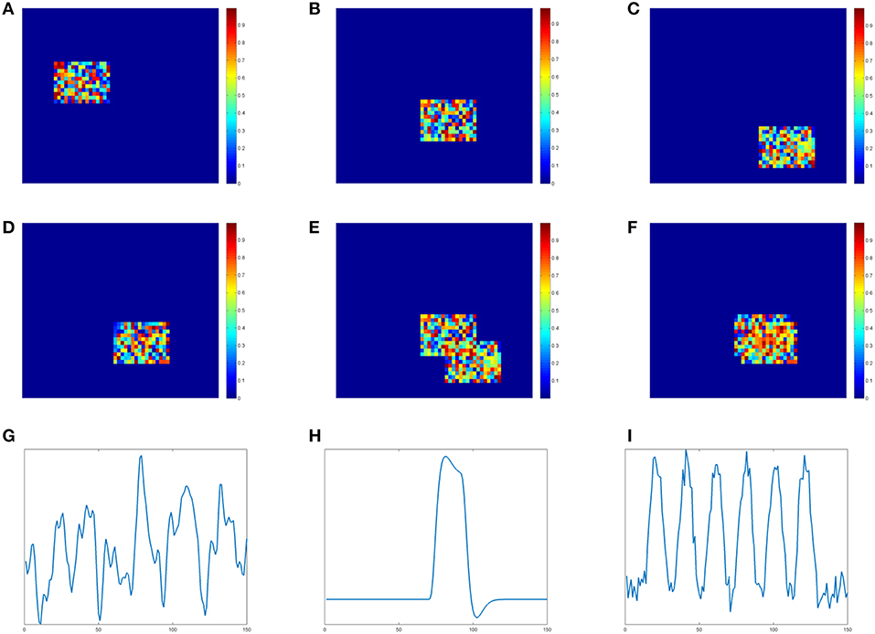
Figure 1. Simulation data of spatial components(SC) and time courses(TC). (A) SC 1. (B) SC 2. (C) SC 3-low overlapping. (D) SC3 high overlapping. (E) SC2&3 low overlapping. (F) SC2&3 high overlapping. (G) TC1. (H) TC2. (I) TC3.

We simulate time courses (TC) using the convolution of the stimulus functions with the hemodynamic response function (HRF) which is generated by SPM function¹ spm_hrf(). We use block design pattern and a single peaked function as the stimulus functions for TC2 and TC3, respectively. TC1 is sampled from time course of real fMRI data [41]. Each TC contains 150 time points and is shown in Figures 1G–I, respectively. These three TCs together form the matrix B with three times courses.

In order to verify the advantage of our proposed algorithm in processing collinearity issue of the subject loading in group ICA, we provide two subject loading matrices C in Equation (23). C₁ is a full rank squared matrix with a low condition number which represents a low collinearity case, while the condition number of C₂ is much higher, which represents a high collinearity case. Each matrix represents 10 different subjects.

$\begin{array}{ll}\begin{array}{cc}C1=& \left(\begin{array}{ccc}2& 2& 3\\ 3& 3& 3\\ 1& 1& 1\\ 1& 3& 3\\ 1& 1& 3\\ 1& 3& 3\\ 1& 2& 1\\ 2& 2& 1\\ 2& 1& 1\\ 2& 1& 3\end{array}\right),\end{array}C2=\left(\begin{array}{ccc}2& 2& 3\\ 3& 3& 3\\ 1& 1& 1\\ 3& 3& 3\\ 1& 1& 3\\ 3& 3& 3\\ 2& 2& 1\\ 2& 2& 1\\ 1& 1& 1\\ 1& 1& 3\end{array}\right).& (23)\end{array}$

We also consider the noise effect to evaluate the robustness of the algorithm. We define the SNR of the data Y as

$\begin{array}{ll}\text{SNR}=\frac{\Vert (C\odot B)A^T{\Vert }_F}{\Vert E{\Vert }_F},& (24)\end{array}$

where E is a matrix with same shape of Y. Each element of E is a random Gaussian noise. We update noised Y using Y = Y + E. The mean of E is 0. The standard deviation σ of E has two values: 0.2 and 0.5. Based on the formula (24), the corresponding values of SNR are about 1.5 and 0.6. Note that a low SNR value means high noise level.

In Table 1, we design eight different tests against three indicators: noise level, overlapping level and collinearity. Each indicator has two contrasting values: low and high. Noise level is evaluated by SNR of the data Y, overlapping level is evaluated by overlapping rate of the shared region, and level of collinearity is evaluated by the condition number of subject loading matrix C. In the next section, we will show the comparison method of these three algorithms and the experimental results.

TABLE 1

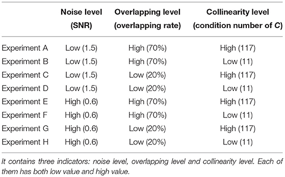
Table 1. Experimental List of Simulation.

4.2. Real fMRI Group Data

We use the data from paper [41] completed at Johns Hopkins University. Data from nine normal subjects were acquired on a Philips 1.5T Scanner. Functional scans were acquired with an echo planar sequence (64× 64, flip angle = 90, TR = 1 s, TE = 39 ms) over a 6-min period for a total of 360 time points. A visual paradigm was designed in which an 8 Hz reversing black and white checkerboard was presented intermittently in the left and right visual fields. The checkerboards were shown for 30 s and were resumed after 60 s. Subjects were focusing on a central cross on the checkerboard during the entire 6 min. The paradigm is depicted in Figure 2. We only have partial data of three subjects instead of nine subjects in this experiment.

FIGURE 2

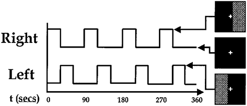
Figure 2. Paradigm used for fMRI experiment. The checkerboards were showed at the high bar period and hid at the low bar period [41].

5. Results

5.1. Simulation Data

We compare four algorithms including TPICA, PARAFAC, Back Construction Algorithm [41], and the proposed Non-Gaussian Penalized PARAFAC. In experiments A-H, we run each algorithm ten times and compare results of SC with the ground truth SC in Figure 1 using congruence coefficient ρ [42], where

$\begin{array}{ll}\rho =\frac{a^{T}b}{\sqrt{(a^{T}a)(b^{T}b)}},\text{given column vectors }a,b.& (25)\end{array}$

Here the value ρ can be used to measure the similarity between the restored component and the truth component. Table 2 shows the means and variances of ρ of spatial sources and Table 3 shows the means and variances of ρ of time courses of each algorithm in each experiment. Figure 3 draws the content of Table 2 in the format of error bars. Then we can compare these four algorithms intuitively.

TABLE 2

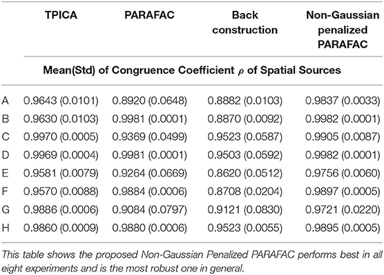
Table 2. Experimental Results of the mean and std of ρ of spatial sources in all four algorithms.

TABLE 3

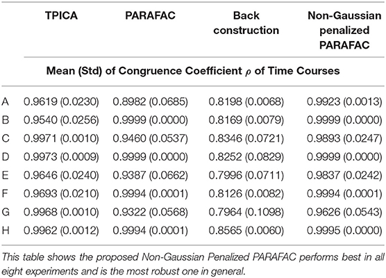
Table 3. Experimental Results of the mean and std of ρ of time courses in all four algorithms.

FIGURE 3

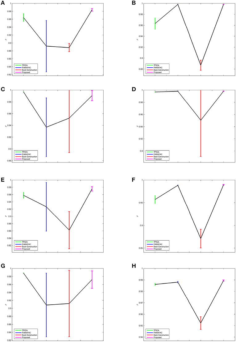
Figure 3. Error Bars of the Experimental Results. The colors of TPICA, PARAFAC, Back Construction Algorithm, proposed Non-Gaussian Penalized PARAFAC from left to right are green, blue, red, and magenta. The vertical axis represents the mean of ρ. The vertical colorful bar represents one std away from the mean value. (A) Experiment A. (B) Experiment B. (C) Experiment C. (D) Experiment D. (E) Experiment E. (F) Experiment F. (G) Experiment G. (H) Experiment H.

In Figure 3, the results of four algorithms in each experiment are showed in one separate subfigure. The horizontal axis shows four algorithms in the order of TPICA, PARAFAC, Back Construction Algorithm, and the proposed algorithm from left to right with the color of green, blue, red, and magenta, respectively. The vertical axis represents the value of ρ. Four vertical error bars represent the intervals of one standard deviation away from the means of ρ.

From Figure 3, it is clear to see that all the assumptions in the previous sections are verified in these eight experiments. (1) The proposed algorithm is the best one compared with TPICA and PARAFAC in all eight experiments. Not only is the mean value of proposed algorithm the highest, but the standard deviation of the proposed algorithm is also the smallest. A higher mean value means a better decomposition, and a lower standard deviation indicates a more stabilized algorithm. Thus, this proposed algorithm overcomes both the collinearity and overlapping issues in this simulation. (2) High noise level can cut down the performances of all algorithms. Experiments (a)–(d) with high level of noise are generally better than experiments (e)–(h) with low level of noise. If the noise level is set to be even higher, it would be very difficult for any algorithm to decompose the data into meaningful components. (3) High collinearity level can dramatically reduce the performance of PARAFAC. Experiments (c) and (g) are typical cases with high collinearity level and low overlapping level. We can see that, in these two experiments, PARAFAC permorms the worst and is not very stable. Adding a non-Gaussian penalty term on the spatial mode can conquer this intrinsic drawback of PARAFAC. (4) High overlapping level can decrease the performance of TPICA although it is still a quite robust algorithm. Experiments (b) and (f) are testing on high overlapping and low collinearity level. TPICA works clearly the worst this time, especially in experiment (d). The independent requirements of ICA hinder any modifications based on itself to deal with the overlapping issue. Thus, we need to modify the algorithm based on PARAFAC in order to avoid this issue.

Figures 4–6 show the decomposition results of the first run of experiments A, B, and C. These figures again verify the above conclusions visually. The time courses in Figures 4–6 are standardized by subtracting their means and divided by their standard deviations. Figure 4 shows the results in the case of low noise, high overlapping and high collinearity. We see that the active regions of SC2 and SC3 of TPICA can not detach from each other very well. One active region of SC includes a light shaded region from another SC. Figure 5 shows the results in the case of low noise, high overlapping and low collinearity. We can see that TPICA performs worst under this situation. The results of time course in TPICA are not very consistent with the truth values and the spatial components in TPICA still have obvious shaded regions around the truth components. Figure 6 shows the results in the case of low noise, low overlapping and high collinearity. This time both TPICA and the proposed algorithm outperform PARAFAC. PARAFAC leads to the degenerate solutions. The first spatial component in the results of PARAFAC is totally meaningless.

FIGURE 4

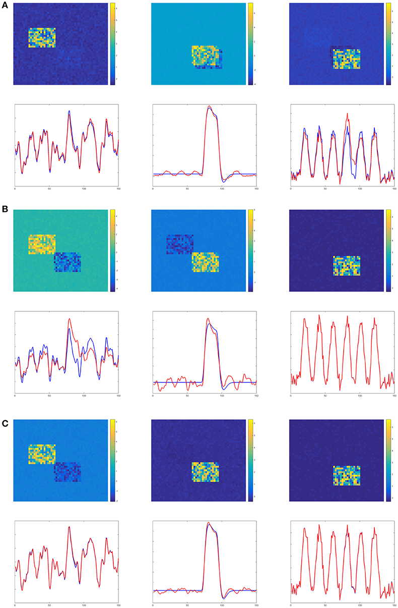
Figure 4. Experiment A in the case of low noise, high overlapping and high collinearity. (A) TPICA. (B) PARAFAC. (C) Proposed Non-Gaussian penalized PARAFAC.

FIGURE 5

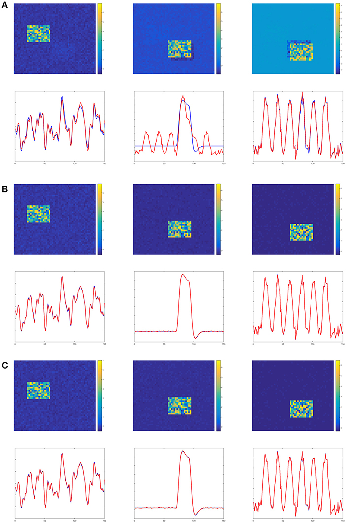
Figure 5. Experiment B in the case of low noise, high overlapping and low collinearity. It shows TPICA suffers from the overlapping issue. (A) TPICA. (B) PARAFAC. (C) Proposed Non-Gaussian penalized PARAFAC.

FIGURE 6

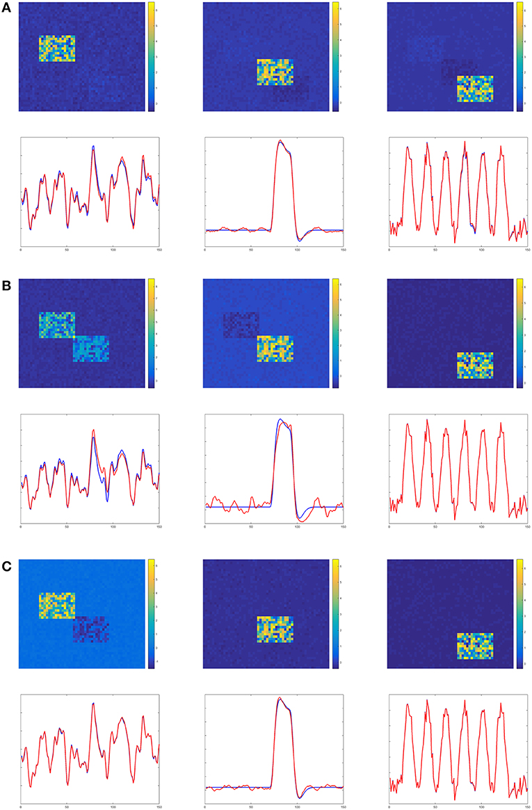
Figure 6. Experiment C in the case of low noise, low overlapping and high collinearity. It shows PARAFAC suffers from high collinearity issue. (A) TPICA. (B) PARAFAC. (C) Proposed Non-Gaussian penalized PARAFAC.

5.2. Real fMRI Group Data

We embed our algorithm into the GIFT package². The final results of the algorithm are summarized in Figure 7, which is generated by GIFT. The threshold value is 2.0 and the slice range is -52:4:8. The activated spatial map shows right visual cortex (blue), left visual cortex (red); a transiently task-related component (TTR, green) in bilateral occipital/parietal cortex. These results are consistent with the results in Calhoun et al. [41], while here we only use three subjects instead of nine.

FIGURE 7

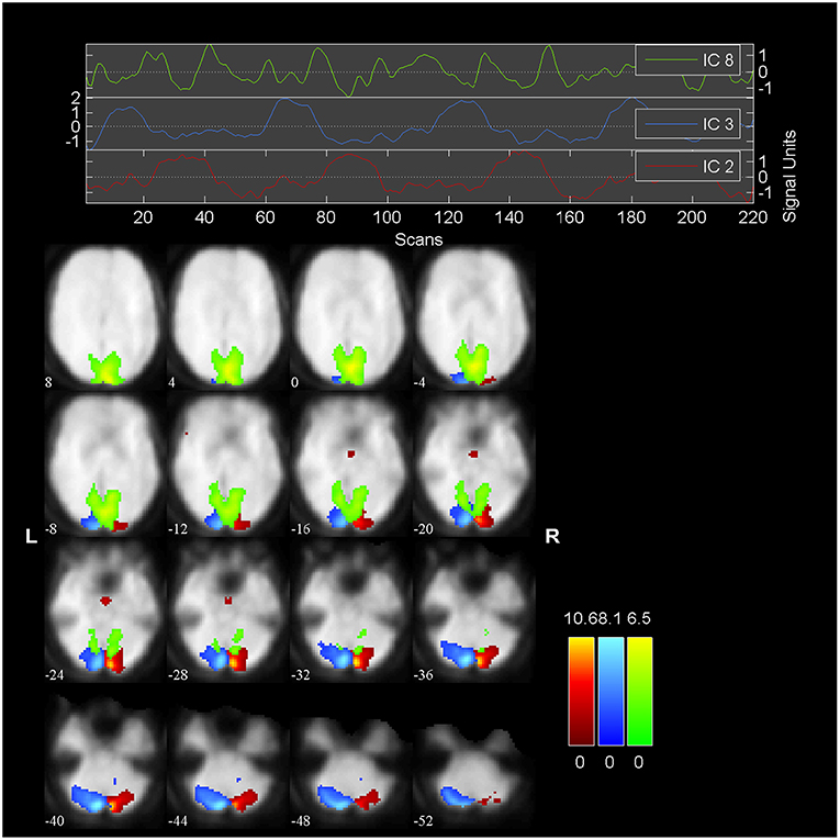
Figure 7. Result of the real fMRI data.

The head part of Figure 7 shows three time courses of the below components. The blue one is the time course of right visual cortex and the red one is the time course of left visual cortex. The peaked and flat periods of two time courses are equivalent to the paradigm in Figure 2 used to control the showing and disappear of the checkerboards in the left and right visual fields.

6. Discussion

In this paper, we successfully alleviate both overlapping and collinearity issues aroused by ICA and PARAFAC by adding a non-Gaussian penalty term to the spatial mode calculation of the PARAFAC. This algorithm can also be deemed as the combination of the characters of ICA and PARAFAC.

The strategy of the fastICA is to project fMRI data onto several orthogonal directions to maximize the non-Gaussianity of the projected data, which are the spatial components. So the assumption of non-Gaussianity is the key character of the spatial components to identify and extract them. The potential degenerate solutions of PARAFAC can be regulated toward the directions (22) of high non-Gaussianity to maximize the proposed object function (21). By this non-Gaussian penalty term, the degenerate solutions could be improved to a good solutions. On the other hand, in the overlapping situation, mutual orthogonal directions calculated by ICA cannot distinguish the correlated spatial components very well. This proposed algorithm is still based on the PARAFAC framework, which does not need the independent constraint of the spatial components. Thus, it can separate the correlated components better than the ICA method.

This proposed algorithm uses the result of fastICA as the initial input. In this way, the algorithm can converge faster and run more robustly than random initial values. Additionally, this better result obtained by this proposed algorithm cannot achieved by either TPICA or PARAFAC no matter how small the tolerance value of the convergence is, how large the maximum iteration time is, and how exact the initial value is. In other words, the improvement of our proposed algorithm is because of the intrinsic modification of the penalty term and cannot be achieved by parameters setting of the other two algorithms. PARAFAC is not robust even when we use the results of TPICA as the initial value.

However, this proposed algorithm is more time consuming than other algorithms due to the calculations of the penalty term and the tensor product. In the future, we can apply the modified PARAFAC using Hadamard products instead of Khatri-Rao products for large-scale problems to overcome this issue [43, 44]. The spatial smoothness and the dependency between spatial and temporal are not considered in this paper, since these two topics are not the primary concerns in designing this algorithm though they are both very interesting topics and can be a problem for further consideration.

Author Contributions

JL, JZ, and DH contributed conception and design of the study. JL performed the statistical analysis and wrote the first draft of the manuscript. JZ and DH improved writing and completed the manuscript. All authors contributed to manuscript finalizing, read, and approved the submitted version.

Conflict of Interest Statement

The authors declare that the research was conducted in the absence of any commercial or financial relationships that could be construed as a potential conflict of interest.

Acknowledgments

The authors are indebted to reviewers for providing insightful and constructive comments and suggestions which has definitely resulted in improvement the readability and quality of the paper. JZ's research was supported by NSFC (No. 61572038) and Chinese State Ministry of Science and Technology (No. 2014ZX02502).

Footnotes

1. ^SPM.https://www.fil.ion.ucl.ac.uk/spm/

2. ^GIFT. http://mialab.mrn.org/software/gift/index.html

References

1. Correa N, Adali T, Calhoun VD. Performance of blind source separation algorithms for fMRI analysis using a group ICA method. Magn Reson Imaging. (2007) 25:684–94. doi: 10.1016/j.mri.2006.10.017

PubMed Abstract | CrossRef Full Text | Google Scholar

2. Calhoun VD, Liu J, Adali T. A review of group ICA for fMRI data and ICA for joint inference of imaging, genetic, and ERP data. NeuroImage. (2009) 45:S163–72. doi: 10.1016/j.neuroimage.2008.10.057

PubMed Abstract | CrossRef Full Text | Google Scholar

3. Allen EA, Erhardt EB, Wei Y, Eichele T, Calhoun VD. Capturing inter-subject variability with group independent component analysis of fMRI data: a simulation study. NeuroImage. (2012) 59:4141–59. doi: 10.1016/j.neuroimage.2011.10.010

PubMed Abstract | CrossRef Full Text | Google Scholar

4. Schmithorst VJ, Holland SK. A Comparison of three methods for generating group statistical inferences from independent component analysis of functional magnetic resonance imaging data. J Magn Reson Imaging. (2004) 19:365–8. doi: 10.1002/jmri.20009

PubMed Abstract | CrossRef Full Text | Google Scholar

5. Assaf M, Jagannathan K, Calhoun VD, Miller L, Stevens MC, Sahl R, et al. Abnormal functional connectivity of default mode sub-networks in autism spectrum disorder patients. NeuroImage. (2010) 53:247–56. doi: 10.1016/j.neuroimage.2010.05.067

PubMed Abstract | CrossRef Full Text | Google Scholar

6. Lindquist MA. The statistical analysis of fMRI data. Stat Sci. (2008) 23:439–64. doi: 10.1214/09-STS282

CrossRef Full Text | Google Scholar

7. Hyvärinen A. Fast and robust fixed-point algorithms for independent component analysis. IEEE Trans Neural Netw. (1999) 10:626–34. doi: 10.1109/72.761722

PubMed Abstract | CrossRef Full Text | Google Scholar

8. Hyvärinen A. Independent component analysis: recent advances. Philos Trans A Math Phys Eng Sci. (2012) 371:20110534. doi: 10.1098/rsta.2011.0534

PubMed Abstract | CrossRef Full Text | Google Scholar

9. Lu W, Rajapakse JC. ICA with reference. Neurocomputing. (2006) 69:2244–57. doi: 10.1016/j.neucom.2005.06.021

CrossRef Full Text | Google Scholar

10. Calhoun VD, Adali T, Stevens MC, Kiehl KA, Pekar JJ. Semi-blind ICA of fMRI: a method for utilizing hypothesis-derived time courses in a spatial ICA analysis. NeuroImage. (2005) 25:527–38. doi: 10.1016/j.neuroimage.2004.12.012

PubMed Abstract | CrossRef Full Text | Google Scholar

11. Lin QH, Liu J, Zheng YR, Liang H, Calhoun VD. Semiblind spatial ICA of fMRI using spatial constraints. Hum Brain Mapp. (2010) 31:1076–88. doi: 10.1002/hbm.20919

PubMed Abstract | CrossRef Full Text | Google Scholar

12. Lu W, Rajapakse JC. Approach and applications of constrained ICA. IEEE Trans Neural Netw. (2005) 16:203–12. doi: 10.1109/TNN.2004.836795

PubMed Abstract | CrossRef Full Text | Google Scholar

13. Formisano E, Esposito F, Salle FD, Goebel R. Cortex-based independent component analysis of fMRI time series. Magn Reson Imaging. (2004) 22:1493–504. doi: 10.1016/j.mri.2004.10.020

PubMed Abstract | CrossRef Full Text | Google Scholar

14. Ma S, Li XL, Correa NM, Adali T, Calhoun VD. Independent subspace analysis with prior information for fMRI data. In: 2010 IEEE International Conference on Acoustics Speech and Signal Processing (ICASSP). Dallas, TX (2010). p. 1922–5.

Google Scholar

15. Sharma A, Paliwal KK. Subspace independent component analysis using vector kurtosis. Patt Recogn. (2006) 39:2227–32. doi: 10.1016/j.patcog.2006.04.021

CrossRef Full Text | Google Scholar

16. Theis FJ. Towards a general independent subspace analysis. In: Proceedings of the 19th International Conference on Neural Information Processing Systems, NIPS'06. Vancouver, BC: MIT Press (2006). p. 1361–8.

Google Scholar

17. Vollgraf R, Obermayer K. Multi dimensional ICA to separate correlated sources. In: Dietterich TG, Becker S, Ghahramani Z, editors. Advances in Neural Information Processing Systems 14. Vancouver, BC: MIT Press (2001). p. 993–1000.

Google Scholar

18. Aapo Hyvarinen POH, Inki M. Topographic independent component analysis. Neural Comput. (2001) 13:1527–58. doi: 10.1162/089976601750264992

CrossRef Full Text | Google Scholar

19. Ge R, Wang Y, Zhang J, Yao L, Zhang H, Long Z. Improved FastICA algorithm in fMRI data analysis using the sparsity property of the sources. J Neurosci Methods. (2016) 263:103–14. doi: 10.1016/j.jneumeth.2016.02.010

PubMed Abstract | CrossRef Full Text | Google Scholar

20. Hyvärinen A. Independent component analysis in the presence of Gaussian noise by maximizing joint likelihood. Neurocomputing. (1998) 22:49–67. doi: 10.1016/S0925-2312(98)00049-6

CrossRef Full Text | Google Scholar

21. Hyvärinen A. Fast ICA for noisy data using Gaussian moments. In: Proceedings of the 1999 IEEE International Symposium on Circuits and Systems (ISCAS 99). Vol. 5. Orlando, FL (1999). p. 57–61.

Google Scholar

22. Beckmann CF, Smith SM. Probabilistic independent component analysis for functional magnetic resonance imaging. IEEE Trans Med Imaging. (2004) 23:137–52. doi: 10.1109/TMI.2003.822821

PubMed Abstract | CrossRef Full Text | Google Scholar

23. Tipping ME, Bishop CM. Probabilistic principal component analysis. J R Stat Soc Ser B. (1999) 21:611–22. doi: 10.1111/1467-9868.00196

CrossRef Full Text | Google Scholar

24. Beckmann CF, Smith SM. Tensorial extensions of independent component analysis for multisubject fMRI analysis. NeuroImage. (2005) 25:294–311. doi: 10.1016/j.neuroimage.2004.10.043

PubMed Abstract | CrossRef Full Text | Google Scholar

25. Guo Y. A general probabilistic model for group independent component analysis and its estimation methods. Biometrics. (2011) 67:1532–42. doi: 10.1111/j.1541-0420.2011.01601.x

PubMed Abstract | CrossRef Full Text | Google Scholar

26. Guo Y, Pagnoni G. A unified framework for group independent component analysis for multi-subject fMRI data. NeuroImage. (2008) 42:1078–93. doi: 10.1016/j.neuroimage.2008.05.008

PubMed Abstract | CrossRef Full Text | Google Scholar

27. Tipping ME, Bishop CM. Mixtures of probabilistic principal component analyzers. Neural Comput. (1999) 11:443–82. doi: 10.1162/089976699300016728

PubMed Abstract | CrossRef Full Text | Google Scholar

28. Bro R. PARAFAC: tutorial and applications. Chemometr Intell Lab Syst. (1997) 38:149–71. doi: 10.1016/S0169-7439(97)00032-4

CrossRef Full Text | Google Scholar

29. Harshman RA, Lundy ME. PARAFAC: parallel factor analysis. Comput Stat Data Anal. (1994) 18:39–72. doi: 10.1016/0167-9473(94)90132-5

CrossRef Full Text | Google Scholar

30. Kolda TG, Bader BW. Tensor decompositions and applications. SIAM Rev. (2009) 51:455–500. doi: 10.1137/07070111X

CrossRef Full Text | Google Scholar

31. Cichocki A. Tensor decompositions: a new concept in brain data analysis. CoRR. (2013) abs/1305.0395.

Google Scholar

32. Cichocki A. Era of big data processing: a new approach via tensor networks and tensor decompositions. CoRR. (2014) abs/1403.2048.

Google Scholar

33. Stegeman A. Comparing independent component analysis and the parafac model for multi-subject artificial fMRI data. In: Invited Speaker at the IOPS Conference (2006). Available online at: http://www.alwinstegeman.nl/docs/Stegeman%20-%20parafac%20&%20ica.pdf

Google Scholar

34. Helwig NE, Hong S. A critique of Tensor Probabilistic Independent Component Analysis: implications and recommendations for multi-subject fMRI data analysis. J Neurosci Methods. (2013) 213:263–73. doi: 10.1016/j.jneumeth.2012.12.009

PubMed Abstract | CrossRef Full Text | Google Scholar

35. Cao YZ, Chen ZP, Mo CY, Wu HL, Yu RQ. A PARAFAC algorithm using penalty diagonalization error (PDE) for three-way data array resolution. Analyst. (2000) 125:2303–10. doi: 10.1039/b006162j

PubMed Abstract | CrossRef Full Text | Google Scholar

36. Stegeman A. Using the simultaneous generalized Schur decomposition as a Candecomp/Parafac algorithm for ill-conditioned data. J Chemometr. (2009) 23:385–92. doi: 10.1002/cem.1232

CrossRef Full Text | Google Scholar

37. Vos MD, Nion D, Huffel SV, Lathauwer LD. A combination of parallel factor and independent component analysis. Signal Process. (2012) 92:2990–9. doi: 10.1016/j.sigpro.2012.05.032

CrossRef Full Text | Google Scholar

38. Eduardo Martínez-Montes JMSB, Valdés-Sosa PA. Penalized parafac analysis of spontaneous EEG recordings. Stat Sin. (2008) 18:1449–64.

Google Scholar

39. Martínez-Montes E, Vega-Hernández M, Sánchez-Bornot JM, Valdés-Sosa PA. Identifying complex brain networks using penalized regression methods. J Biol Phys. (2008) 34:315–23. doi: 10.1007/s10867-008-9077-0

PubMed Abstract | CrossRef Full Text | Google Scholar

40. Martínez-Montes E, Sarmiento-Pérez R, Sánchez-Bornot JM, Valdés-Sosa PA. Information entropy-based penalty for PARAFAC analysis of resting EEG. In: Wang R, Shen E, Gu F, editors. Advances in Cognitive Neurodynamics ICCN 2007: Proceedings of the International Conference on Cognitive Neurodynamics. Dordrecht: Springer (2008). p. 443–446.

Google Scholar

41. Calhoun VD, Adali T, Pearlson GD, Pekar JJ. A method for making group inferences from functional MRI data using independent component analysis. Hum Brain Mapp. (2001) 14:140–51. doi: 10.1002/hbm.1048

PubMed Abstract | CrossRef Full Text | Google Scholar

42. Tucker LR. A method for synthesis of factor analysis studies. In: Technical Report 984. Princeton, NJ: Educational Testing Serice (1951).

Google Scholar

43. Phan AH, Tichavsky P, Cichocki A. Fast alternating LS algorithms for high order CANDECOMP/PARAFAC tensor factorizations. IEEE Trans Sig Process. (2013) 61:4834–46. doi: 10.1109/TSP.2013.2269903

CrossRef Full Text | Google Scholar

44. Phan AH, Cichocki A. PARAFAC algorithms for large-scale problems. Neurocomputing. (2011) 74:1970–84. doi: 10.1016/j.neucom.2010.06.030

CrossRef Full Text | Google Scholar