Recent Developments in the Dynamic Stability of Elastic Structures

1. Introduction

The topic of dynamic stability, or to put it in Bolotin terms “dynamic instability” [1], is inherently a highly multidisciplinary problem, impacting a wide variety of fields (mathematics, engineering, chemistry, biology, ecology, economic, etc.). This review focuses on engineering applications with particular emphasis on elastic structural systems. This issue has attracted significant scientific interest, beginning with the first rigorous definition of stability provided by Aleksandr Mikhailovic Lyapunov at the end of the nineteenth century [2]. Despite its relatively long tradition, the dynamic instability of elastic systems has yet to be fully explored, and several highly topical issues still await clarification.

Dynamic instability phenomena, in contrast with their static counterparts, take place at a non-zero critical frequency and involve all mechanical problems in which the inclusion of time cannot be avoided. This is the case for structural mechanical systems subjected to a dynamic loading in their equilibrium state: either, where the load applied is sudden (e.g., shock, impact loading etc.), or in the case of aero- or hydro-elastic forces, or pulsating parametric forces, or follower forces, and so on [3–6]. Dynamic stability issues may also affect systems whose post-critical response is a dynamic process, and/or systems that are in motion in their unperturbed state. It is important to highlight that all real-world stability problems are dynamic, although they can be successfully modeled as static.

The present review cannot be seen as a thorough survey of the dynamical stability of mechanical systems. This would be an impossible task, and beyond the scope of a single article. The research literature is too extensive, and the issues too many. For a more complete understanding, the reader is referred to the countless textbooks that have been written on the topic [1, 2, 4–11]. Rather, the attempt here is to focus on current issues and trends, while giving an overview of the pertinent literature, with special emphasis on some relevant outstanding topics. The paper will proceed as follows. Section 2 briefly discusses the fundamental concepts in static and dynamic stability, including a short summary of both local and global bifurcations, and of chaos (section 2.2). Section 3 focuses on the difference between linear and non-linear instability, highlighting some misleading interpretations of the dynamic response of a mechanical system caused by linearization near a fixed point. Sections 4 and 5 present two different methods—the primary analytical/semi-analytical method, and the numerical method—that are used to solve equations governing the dynamic stability of structures. Section 6 emphasizes the strong sensitivity of dynamic systems, including a presentation of the main techniques used to address this problem. A paradigmatic example on the destabilizing effect of small vanishing damping (Ziegler paradox) is also given. Section 7 reviews some experimental investigations, with emphases on experimental developments in follower-forces, while section 8 reviews some recent developments in innovative smart applications. Section 9, finally, contains concluding remarks, highlighting the necessity of intensifying experimental investigations into post-buckling behavior in order to close the gap between analytical and experimental studies.

2. Fundamentals of Stability

Instability phenomena that take place at zero natural frequency are known as static. These encompass problems that involve path-independent forces (e.g., conservative forces) and more generally all problems where load is applied in a static or quasi-static manner. Vice versa, the term dynamic instability refers to a large class of problems and several different physical phenomena which require the inclusion of time. Examples of dynamic instability in structural mechanics include [1, 12]:

i. parametric resonance. Instabilities of periodic motions (i.e., parametrically excited vibrations) can be occur when a structural system is loaded by periodic (i.e., time-varying) excitation; or the system parameters are periodically modulated. In such cases, the system experiences parametric resonance [13–15]: an equilibrium point becomes unstable, and any even small perturbations involve large amplitude oscillations. A classic example of this phenomenon is a person on a swing, which can be modeled as a pendulum of varying length [16]. A considerable amount of research and reviews have been carried out on this topic. Most deal with pulsating forces that result in the parametric resonance of columns, shallow arches, or shells. Others deal with internal parametric excitation and with the parametric resonance that occurs in fluid-solid interaction problems [17, 18]. Finally, several studies have employed parametric resonance in micro-electro-mechanical systems (MEMS) (see [19] and references therein).

ii. Instabilities under the sudden loading of conservative systems. These include a large number of dynamic problems (e.g., arches and arch-like structures, shells, and initially curved panels) in which the structures are either loaded with a large integral impulse and vanishingly small duration loads (e.g., by impact load), or suddenly loaded with constant magnitude and infinite duration loads. In such cases, the critical state that corresponds to quasi-static loading degenerates in a limit point, with the loss of stability resulting in a codimension-2 bifurcation (i.e., snap-through buckling). In such cases, the transition, or “jump” to another non-adjacent equilibrium point is a dynamic process. The first to tackle these issues were Hoff and Bruce [20], who in the early 1950s proved the dynamic buckling of flat arches under lateral sinusoidal loading by investigating Total Potential Energy. Their pioneering paper led to significant interest in stability issues associated with shallow arches over the reminder of the twentieth century. Important research contributions were also made by other outstanding scientists. Budiansky and Roth [21], for instance, investigated a suddenly loaded shallow spherical shell with axisymmetric behavior by numerically integrating the motion equations. Simitses [22], meanwhile, analyzed the snap-through behavior of low arches and shallow spherical caps. And Hsu [23–25] produced a qualitative investigation of the trajectory of the motion in the phase-plane (Total Energy-Phase Plane Approach). The book [4] contains a survey of some relevant results achieved on the subject.

iii. Instabilities in non conservative systems [6, 11]. In a large number of engineering applications, the forces are statically applied but the system is non-conservative. This is the case for follower-force problems, rotating shafts (whirling), and aeroelasticity instability (i.e., fluid-solid interaction and flutter). Some of these problems (e.g., the follower-force problem) exhibit two different types of unstable behavior: divergence and flutter instabilities. Divergence instability is a typical quasi-static-bifurcation leading to an exponentially growing motion. Flutter instability, conversely, is a typical dynamic instability leading to the absorption of energy from a steady source by means of self-sustaining oscillations. Divergence instability can be determined by classical approaches (i.e., a classical, quasi-static bifurcation technique, potential energy, or kinetic energy methods). Flutter instability, meanwhile, is only detectable using dynamic analysis. This last observation has given rise to an amount of paradoxes in the last century, the most famous of which is the destabilization effect due to small damping (Ziegler paradox [26, 27]), which is described in detail in section 6.1. Rotor-dynamic instability, conversely, leads to unstable torsional and whirling vibrations that were recognized by Crandall [28]. The rotors' dynamic behavior is affected by their filling ratio, the effect of surface oscillations (i.e., the sloshing motion) of the rotating liquid, and also by damping which in this context has a destabilizing effect. Flow-induced instabilities are a fascinating topic pertinent to aircraft, spacecraft, airfoil, nuclear power plants, conveying pipes, etc. Fluid-solid interaction leads to panel flutter instability, divergence and parametric resonance. The issue has been widely explored in the literature, notably in light of the notorious collapse of Tacoma Narrow Bridge near Seattle in 1940.

2.1. Stability Criteria

Due to the great variety of phenomena that encompass instability, it is not possible to provide a universal way of looking at stability. Depending on the nature of the problem, three main approaches and three ensuing criteria can be employed to assess the stability of a structure's equilibrium: the equilibrium method (static approach) proposed by Euler, the energy method and the dynamic method. All three above-mentioned methods are independent, meaning that the results that they provide may not always be comparable. The equilibrium method investigates the existence of a non-trivial equilibrium state infinitesimally close to the initial one. From a mathematical point of view this is equivalent to investigating the existence of non-trivial solution for the equilibrium equation of the perturbed system. The existence of at least one more neighboring equilibrium state implies that the equilibrium configuration of the elastic body is unstable. It is important to stress that the equilibrium method provides non-trivial solutions only in the case of non-linear elasto-static problems. Furthermore, if there are non-conservative forces (e.g., follower forces) it can give paradoxical and erroneous results, so its applicability is restricted to conservative systems. Finally, it is general unable to detect so called snap-through instability (the typical instability of shallow arches and domes) and dynamic flutter instability.

The energy method can be applied, more generally, to systems where an energy functional exists (e.g., conservative mechanical systems). It is based on the Lagrange-Dirichlet theorem which states that the equilibrium locus of a conservative system with holonomic and scleronomic constraints will be stable if and only if the total potential energy ${E}$ (the sum of potential energy of deformation and strain energy) takes a minimal value in the class of virtual displacements (i.e., infinitesimal displacements satisfying kinematical constraints). Accordingly, for any optional but sufficiently small deviation from an equilibrium state the stability points are associated with the stationarity of the second variation of the total potential energy ${\partial }_2{E}$. Figure 1 provides a very illustrative graphical representation of this approach: the structure is modeled as a ball which is initially in balance on an energy surface. When a small perturbation is applied the ball moves from its equilibrium position. Generally, three cases can arise. In the first case, the ball is in equilibrium at the lowest point of a concave surface, moving away from its equilibrium point and then releasing, it will roll back toward the position of minimal potential energy and the equilibrium will be stable (Figure 1A).

FIGURE 1

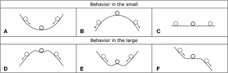
Figure 1. Simple illustrative representation of stable, unstable, and indifferent equilibrium positions in the small (A–C) and in the large (D–F). The arrows represent admissible perturbations.

In the second case, the ball is on top of hump, as shown in Figure 1B, and the stationary point has a maximal potential energy. Accordingly, moving away from its equilibrium position and releasing, the ball rolls farther away from equilibrium and the equilibrium will be unstable. Finally, when the ball is located on a flat surface and it is moved away from its original spot, it adopts a new different equilibrium position (Figure 1C) without any change in potential energy. In this case the equilibrium is said to be indifferent. It is necessary to stress that this stability criterion is only a local in scope, because a large perturbation can lead to stability in the small and instability in the large [e.g., in the case shown in Figure 1D a large perturbation sends the ball over the small hump definitively removing it from the stationary point] or vice versa (Figure 1E).

The process through which the structure (i.e., the ball) returns to (or moves away from) its current state is a time-dependent process and should be treated as such (i.e., dynamically). A dynamic approach provides a much more complete insight into static instability problems as it enables the computation and tracking of the complete state vector (i.e., displacement and velocity fields) and yields accurate information on the post-buckling response of the structure.

The dynamic method is a more general approach which can be used to investigate static and dynamic stability alike. It is based on the classical definition of stability which goes back to Lyapunov (the so-called two-metric stability of Lyapunov) which states that a necessary and sufficient condition for stability of an equilibrium point is that all solutions of the evolution equations that govern the problem starting nearby initial conditions remain close to this state all the time. In terms of phase space this can be geometrically interpreted as follows: once a sphere however small in radius ε > 0 is chosen around the equilibrium point x^*, it is always possible to construct another sphere of radius δ(ε) that is contained in the ε-sphere (Figure 2). All the trajectories x(t) with its origin in the δ-sphere will remain in the ε-sphere when the time increase and will never reach its limit.

FIGURE 2

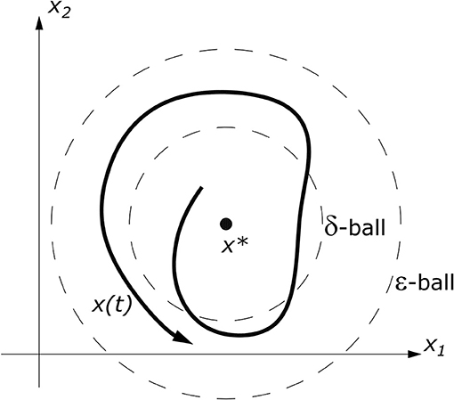
Figure 2. Geometric interpretation of stability in the sense of Lyapunov.

The interested reader can find a more in-depth and detailed description of the concepts presented in this Section in references [29–34].

2.2. A Brief Survey of Static and Dynamic Bifurcations

By slightly varying one or more system parameters, the qualitative behavior of solutions can abruptly change, resulting in bifurcations [7, 8]. Equilibria can then be created or destroyed. Periodic, quasi-periodic, homoclinic, heteroclinic, or chaotic dynamics may also appear. In a static problem, three different types of codimension-1 bifurcations of static equilibria can occur (Figure 3):

i. transcritical bifurcation (also known as exchange of stability) whereby a stable and an unstable point of equilibrium coalesce at the asymmetric point of bifurcation and then re-emerge, switching their stability;

ii. saddle-node bifurcation whereby two equilibria move toward each other, collide and finally annihilate one other;

iii. supercritical or subcritical pitchfork bifurcation. Supercritical pitchfork bifurcation is also known as safe bifurcation, whereby two non-zero symmetrical equilibrium points appear at small amplitude. Subcritical pitchfork bifurcation, meanwhile, is also known as dangerous bifurcation as it results in a leap from zero to large amplitude. The latter is common in the buckling of symmetrical arches [10].

FIGURE 3

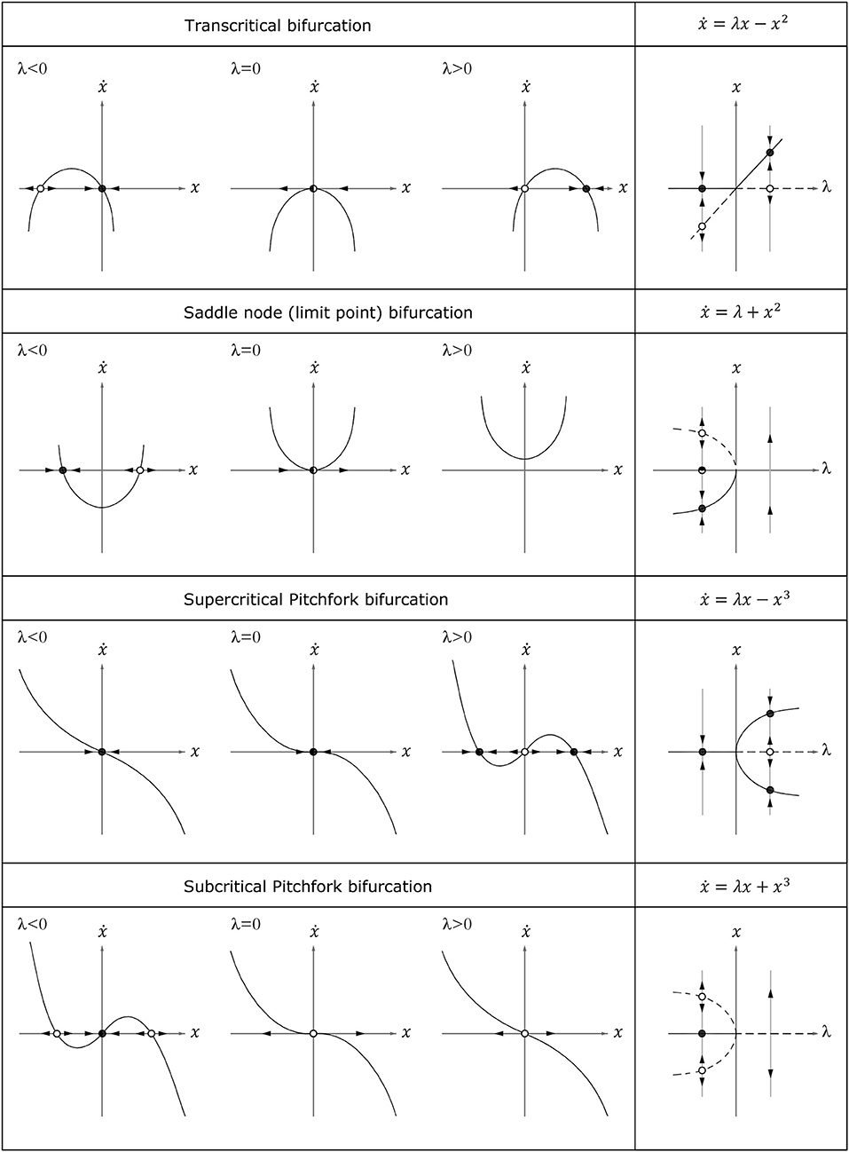
Figure 3. Phase portrait evolution by changing the parameter λ (left) and bifurcation diagram corresponding to the normal form (right).

All the above bifurcations are local, in the sense that they involve the degeneracy of some eigenvalues of the Jacobian matrices associated with fixed points.

Moreover, when real-world circumstances cause imperfections to break the symmetry, a limit point (i.e., a maximum point of the load-path) can be reached [9], leading to snap-through instability. This is also known as codimension-2 cusp bifurcation. In such cases, the instability behavior is controlled by two independent parameters: the beam lateral deflection and the imperfection amplitude to name just an illustrative example. At the limit point, the structure abruptly “jumps” in a distant stable equilibrium state, leading to large amplitude displacements and a potentially catastrophic event for the structure's equilibrium. This impressive static bifurcation for a shallow elastic arch is sketched in Figure 4.

FIGURE 4

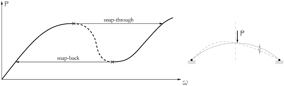
Figure 4. Codimension-2 cusp bifurcation of a shallow elastic arch. Unless otherwise stated, continuous and dashed lines represent stable and unstable equilibria, respectively.

In the case of dynamic stability, the emergence of a trace of limit cycles rather than a static equilibrium path (Figure 5) leads to more complex types of local fixed point bifurcations [10, 35]. These include:

iv. cyclic fold (tangent) bifurcation whereby two limit cycles (stable and saddle) approach each other along the unstable manifold as a control parameter changes, then collide at the bifurcation and disappear with a bang (snap-through phenomenon). In terms of the eigenvalues of the Jacobians associated with cycles, this is a zero-eigenvalue bifurcation (i.e., the bifurcation occurs when one of the eigenvalues equals zero);

v. Hopf bifurcation whereby a pair of complex conjugate eigenvalues crosses the imaginary axis of the complex plane from left to right as the values of the control parameter increase from negative to positive, then sinks to become a saddle. As in the case of pitchfork bifurcation, it can be sub-critical or super-critical, resulting in stable or unstable closed orbits, respectively;

vi. Flip (periodic-doubling) bifurcation of cycles whereby a stable limit cycle loses its stability at the same time as a new closed orbit (either super-critical or sub-critical) arises, featuring a double period with respect to the original cycle;

vii. Neimark-Sacker (secondary Hopf) bifurcation of cycles whereby a limit cycle loses its stability, giving rise to an attracting two-dimensional invariant torus T². In this case, a pair of complex conjugate eigenvalues crosses the unit circle in the complex plane. On the torus are located long-period cycles of different stability types.

FIGURE 5

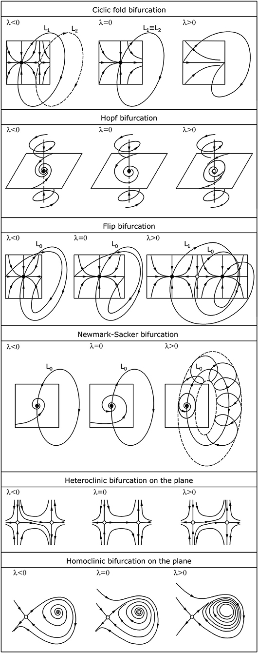
Figure 5. Phase portrait evolution by changing the parameter λ of local and global dynamic stability.

The first two bifurcations typically occur in second-order systems, while the last two can occur only in systems of an order greater than or equal to three. In addition to these bifurcations there are the so-called global bifurcations of cycles that involve large regions of the phase plane:

viii. heteroclinic bifurcation, in which all the solutions migrate from one saddle point to the other, including heteroclinic cycles;

ix. homoclinic bifurcation as an infinite-period bifurcation in which part of a limit cycle moves increasingly close to a saddle point, before touching it the bifurcation, becoming a homoclinic orbit.

In this instance, however, investigating the behavior of the system via a single fixed point provides only partial information about the system's overall behavior.

Another fascinating possibility for a dynamic system is that a slight variation in a control parameter elicits a catastrophic transition toward a different attractor. The transition may take place from cyclic to quasi-static, or even in chaotic regimes (route to chaos). The latter is true in the case of the Šilnikov bifurcation and the Feigenbaum cascade [36]. The Šilnikov bifurcation is a homoclinic bifurcation that triggers the collision in a three-dimensional state space of a saddle cycle and a stable torus, leading to the so-called “torus explosion.” The Feigenbaum cascade is an infinite collection of period doubling bifurcation connected to each other by periodic orbits in a pattern known as a “cascade.”

3. Linear vs. Non-linear Theory

In a structural system non-linearity can arise from a number of causes, including geometry (e.g., large displacements and/or rotations, curvature, shape etc.), material properties (i.e., nonlinear stress-strain relations) and structural damage (e.g., breathing cracks [37]).

The well-known Hartzman Grobman theorem [38] describes the topological equivalence between the local phase portrait near a hyperbolic fixed point and the phase portrait of a linearized system

$\begin{array}{ll}\dot{x}=f(x,\lambda )=f_0(\lambda )+f_1(\lambda )x+f_2(\lambda )x^2+o(x^3)& (1)\end{array}$

(i.e., there is homeomorphism from one phase portrait to the other). In view of this statement, many non-linear instability problems can be easily addressed using linear analysis. However, the geometric non-linearity of large deflection as well as physical or constructional non-linearities play a detrimental role in determining the actual stability limit of both conservative and non-conservative systems. The phase portrait and the time-amplitude diagrams of two basic types of bifurcations instability (saddle point divergence instability and flutter instability) in Figure 6 illustrate this point. The figure clearly shows how linearization can induce a misleading interpretation of the static or dynamic behavior. In both cases, a bounded stable response in the large is misinterpreted as an unbounded unstable response by linear investigation [39]. Moreover, in the case of flutter instability, the linear analysis fails to detect new attractors, such as stable limit cycles, as is the case in the well-known Beck problem [40, 41], the Nicolai paradox [41, 42], and the Ziegler paradox [26, 27] (further details on the latter are discussed in the section 6.1 of this paper).

FIGURE 6

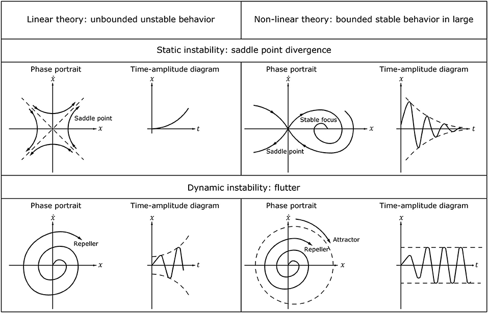
Figure 6. A comparison between linear and non-linear investigations of static and dynamic bifurcations.

To summarize, as the effect of “turning on” the higher-order terms in the normal form involves a violation of non-degeneracy condition of non-linear terms (i.e., some Lyapunov coefficients do not vanishing at the critical point) the phase portrait is qualitative alterated. Therefore, the truncated normal form is not able to capture all essential events on the behavior for the global system and “strange” dynamics. This is the case of the so-called “degenerate bifurcations” (e.g., codimension-2 cusp, Bautin and Bogdanov-Takens bifurcations). They are undetectable by monitoring only the eigenvalues but we have to take into account the higher-order Taylor series coefficients of f(x, λ) at the equilibrium. Clarifying examples of beams, plates and thin-walled structures in which the eigenvalues analysis obscures the possibility of multiply compound branching behavior and potentially dangerous post-buckling behavior are included in Guarracino [43] and Guarracino and Walker [44].

In the context of non-linear behavior of structures under dynamic loading in addition to the more traditional direct problem, another issue worth of attention is the inverse bifurcation problem of determining model parameters to result in certain desired values of the external parameters (see [45, 46] and references therein). The key idea is to map the bifurcation manifold back to the space of parameters. In so doing, it serves two purposes: firstly, for a given set of external parameters, the identification of the parameter configurations that lead to a specific property or interesting dynamics (bifurcation control problem); secondly, the design of system parameters in such a way as to ensure the desire qualitative outcome (bifurcation prediction problem).

4. Analytical and Semi-analytical Methods

The stability problem for dynamic system is generally governed by non-linear Partial Differential Equations (PDEs). In very limited and clearly defined cases such problems may be solved in closed analytical form; for example, by solving the transcendental equation of stability that is associated to the integration of differential equations of stability [47, 48]. This leads to a non-linear eigenvalue problem that, most of the time, it is preferred approximate by a linear eigenvalues problem. The first theoretical predictions of dynamic buckling loads were conducted by Hoff and Bruce [20]. They provided the dynamic buckling of flat arches under lateral sinusoidal loading. Techniques by which to integrate the equations governing the study of the stability of equilibria and periodic orbits include various analytical and semi-analytical methods. Their applicability is, however, limited and strongly dependent on the involved parameters. A short survey of these methods is given below.

i. The perturbation method is an approximate direct technique that provides the solution for weakly non-linear problems and the associated boundary conditions in form of a small parameter power series (i.e. a perturbation series) [49]. The heavy dependence on physical parameters is its greatest drawback, and as such it is entirely unsuitable for strongly non-linear problems. Combined methods (i.e. semi-analytical methods) first of all approximate the unknown displacement field by polynomial or coordinate functions, then analytically solve the discretized governing PDEs (i.e., the obtained set of non-linear ordinary-differential equations).

ii. One such method is the traditional Taylor expansion method. By appropriately adjusting the number of terms of the series expansion and the step-size, it provides a highly-accurate and stable solution in terms of unknown higher-order derivatives. It is hence particularly suitable and useful when the analyzed problem requires both long-time numerical simulations and high-levels of solution accuracy. However, this method requires an increasing amount of computational effort as the system dimension increases.

iii. The semi-analytical Adomian Decomposition Method (ADM) gives a solution for PDEs in a polynomial form, by employing the so-called “Adomian polynomials.” The major advantage of the ADM is that it provides a simple algebraic system of equations to solve [50].

iv. The Homotopy Analysis Method (HMA) provides solutions for highly non-linear stability in the form of analytical expressions (i.e., convergent series). This significantly increases the convergence speed for the solutions. The method, which is independent of small parameters, is very efficient and simple. It has thus been widely utilized in recent literature addressing snap-through issues [51]. Both here and in the ADM method, solution convergence can be obtained without the need to linearize the stability equations.

v. Another proven approach for determining the critical load of elastic structures is phase plane/space analysis. This method involves the topological characterization of the stability boundary (i.e., the locus of equilibrium points and periodic orbits in the parameter space).

vi. In the special case of conservative loads, stability can be assessed, alternative, by using the well-known Lagrangian-Dirichlet and Lyapunov theorems [31, 52]. By pursuing the energy based approach, a lower conservative bound of the critical load can be obtained by leaving non-linear equations of motion unsolved [53, 54]. The solution of variational energy governing equations generally follows a step-wise procedure (Rayleigh-Ritz method, Galerkin method, etc.). The drawbacks of an energetic approach are, on one hand, the overly conservative buckling load, and, on the other, the impossibility of including rigorous damping effects, even though these can have a significant effect on the stability of a structure [55, 56].

5. Numerical Methods

The main focus of the study of dynamic systems is the detection, analysis and continuation of their equilibria (i.e., limit cycles, homoclinic, and heteroclinic orbits), as well as tracing the associated bifurcation diagrams. An analytical approach is generally preferred, as it offers a quick, exact solution. Without numerical calculations, however, this is an arduous or sometimes non-viable task in view of the complexity of bifurcation boundaries, especially when dealing with multi-dimensional systems and strongly non-linear stability problems. A numerical approach, conversely, provides more general, albeit approximate, solutions to the stability problem. It significantly reduces integration times and allows for parametric studies. It also enables the physics of very complex problems to be taken into account, providing accurate results for a relatively high computational effort [57].

The equilibria, i.e., the solutions of the ODE's associated to the stability problem

$\begin{array}{ll}\dot{x}=f(x),x\in ℝ& (2)\end{array}$

can achieve fairly accurate predictions via numerical integration. When the load approaches a fixed point, the stiffness matrix become ill-conditioned. This can then be used as a constraint by which to obtain the critical points, in addition to the governing equations. Much attention has been given to this issue, including incremental-iterative procedures. These are generally based on Newton's method with its modifications (e.g., the Newton-chord and -secant method, Newton-Kantorovich method, etc.), or the Broyden method, path-following techniques, and continuation methods, such as the arc-length continuation method [10, 33, 58, 59]. Searching limit cycles is, however, a more difficult task. In the literature, this problem is generally formulated as a periodic Boundary-Value Problem (BVP) on a fixed interval that is solved using various numerical approaches under differing assumptions:

i. The shooting time-stepping method (i.e., multiple or parallel shooting) [60] is a simple and effective iterative method. From an initial estimate, it computes continually-improving approximations of the solution to an evolution problem. This is a very general approach that replaces the considered boundary-value problem with an equivalent initial value problem. To do this, the time interval is split into a number of sub-intervals. Subsequently, the underlying initial value problem is solved at every time increment. However, the convergence of the method cannot always be ensured, and in some cases (e.g., when the problem is highly sensitive to the initial conditions, or when the Monodromy matrix has widely separated eigenvalues in the interval over which the integration is carried out) a machine overflow can occur.

ii. The finite difference (FDM) and finite element methods (FEM) [60, 61] are a very popular way to study stability problems, especially those involving geometric non-linearity. The key idea underlying all FDMs is to approximate, point-wise, the derivatives in the differential equations by finite difference equations. In this manner, the system of partial differential equations (PDEs) that govern the problem results into a system of simultaneous algebraic equations which is typically solved by means of iterative methods (e.g., Gauss-Seidel method, Jacobi method, and many others). FDM is a very simple discretization method for understanding and applying and it can be applied to fairly difficult problems. However, it may run into difficulty, when the problem is non-linear. Indeed, non-linearity in differential equations results in a large algebraic system which is in turn non-linear, this leads a large computational effort.

The FEM is versatile and widely-used method, particularly suitable for problems with complex geometries. It yields an approximate solution of the differential equations by discretizing the global solution domain into a number of sub-domains (i.e., elements). A solution is found at a finite set of points by means of several methods (Rayleigh-Ritz method, Galerkin weighted residual method, etc.). Trial functions (i.e., finite elements) are defined on each element; they are nonzero only in that element and zero everywhere else. The resulting piecewise approximation is substituted in the original differential equation leading to an algebraic system of equations.

iii. The Differential-Quadrature Method [62] is a recent mesh-less technique for solving partial and total differential equations which offers a compelling alternative to the conventional finite difference and finite element methods. This method replaces partial derivatives in the differential equations with weighted sum of function values at all the discrete points (mesh points) of global domain. Due to the independence of the variational principles, this method is simple both in terms of mathematics and programming. Although it can be a computationally expensive technique, it provides highly accurate solutions.

Other frequently used numerical methods seen in the literature are the so-called differential transformation-based element method, and Reduced-Order Models (ROM). Most modern software packages are focused on bifurcation analysis. The most well-known of these are AUTO [63] and LOCBIF, which are especially suited to detecting global and local bifurcations, respectively. CONTENT [64] and MATCONT [65] are also worthy of mention here.

6. Imperfection Sensitivity

Generally, dynamic stability problems exhibit extreme sensitivity to slight geometrical (overall and or cross-sectional defects), loading imperfections, thermal stresses, and even vanishing, but non-zero, damping forces (for further details, see the section 6.1). As their structural behavior can be strongly affected by sensitivity, the first limit point is approached considerably earlier than the bifurcation load in the imperfect structure compared with the perfect structure. This results in a significant drop in load carrying capacity and large out-of-plane displacements. It is hence necessary to properly take account of the effects of imperfections on the stability in the design process. The critical state sensitivity analysis has been frequently discussed in the past. Recently a number of authors have used a range of approaches to address the problem [66] Among the methods that allow the effects of structural imperfections to be taken into account, the following are especially noteworthy:

i. The Koiter-Newton method is a step-by-step method that combines a non-linear reduced order model (ROM), based on Koiter's initial post-buckling expansion, and the Newton arc-length correction method. The resulting algorithm provides a very accurate and efficient equilibrium path, even when buckling is present and/or the structure is imperfect [67].

ii. Incremental-iterative methods [59] make it possible to directly determine (i.e without tracking the equilibrium paths of imperfect structure) the limit points and simple or multi-bifurcations of parameterized structures in the entire parameter space, via an incremental-iterative (predictor-corrector) algorithm. The latter combines a load incremental scheme with an iterative scheme (e.g., arclength method will be used for load incremental scheme and minimum residual displacement method will be used for iterative scheme). However, methods such as this lead to errors that do not increase with the parameter values and are therefore often preferred to perturbation approaches.

iii. Perturbation analysis [68] provides a direct methodology for investigating the sensitivity to structural imperfections in bifurcation problems. The perturbation surrounding the critical point is examined for both equilibrium equations and the critical constraint.

iv. The Lyapunov-Schmidt-Koiter asymptotic approach [69] relies on the Lyapunov-Schmidt decomposition and Koiter's asymptotic expansion about the bifurcation point. An effective and reliable approach that is suitable for elastic structures under conservative loading, it is able to provide not only an accurate equilibrium path but also the least desirable imperfection shapes.

Both of these two latter approaches offer the possibility of fully automated implementation through the finite element method, and provide highly accurate results. However, their validity is limited to a very small range around the bifurcation or the limit point.

6.1. The Effect of Damping: A Paradigmatic Example

In the past, the buckling problem under follower forces was frequently addressed using the equilibrium method, which goes back to Euler [70] (i.e., investigating the existence of an adjacent non-trivial equilibrium state). This has led to many ambiguities, paradoxes and errors [41].

One of the best-known paradoxes is the so-called “Ziegler paradox” [26, 27]. This concerns the sensitivity of the stability of the upward double pendulum depicted in Figure 7 to vanishing (non-zero) damping forces. As long as it is undamped, this system is stable for a wide range of loads. However, it becomes unstable as soon as the slightest damping is observed. Since its discovery by Ziegler in 1952, this paradox has attracted extensive attention from researchers [26, 27, 41]. Worthy of note is the fascinating explanation on dissipation-induced instabilities provided by Kirillov and Verhulst in their recent work [71]. They stated that the destabilization of the system by small dissipation is closely related to Whitney umbrella singularity emerging on the stability boundary. Ziegler's pendulum consists of a two-degrees-of-freedom double-rod system with concentrated elasticity and inertia. This is subjected to a follower force F acting in the axis of the second bar. The system consists of two visco-elastically hinged rigid bars of length ℓ₁ and ℓ₂. The inertia and the elasticity of the system are provided by two lumped masses m₁ and m₂, which are located at the middle of each bar, and by two rotational springs of stiffness k₁ and k₂ and mechanical linear damping coefficient c₁ and c₂ (all positive and real quantities), respectively. The evolution of the system in time (t) is unequivocally defined by the Lagrangian parameters φ₁(t) and φ₂(t) (i.e., the rotation angles that the two rods form descending the vertical axis).

FIGURE 7

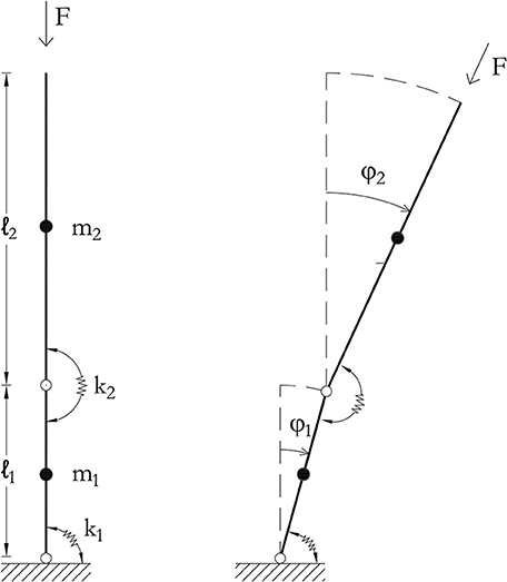
Figure 7. The Ziegler double pendulum.

The non-linear dynamic motion equations are easily derived from the well-known Euler-Lagrange equation

$\begin{array}{l}\left(\frac{m_1{\ell }_1^2}{4}+m_2{\ell }_1^2\right){\ddot{\phi }}_1+\frac{m_2{\ell }_2{\ell }_1}{2}cos\left({\phi }_2-{\phi }_1\right){\ddot{\phi }}_2+\left(c_1+c_2\right){\dot{\phi }}_1\\ -c_2{\phi }_2+\frac{m_2{\ell }_2{\ell }_1}{2}sin\left({\phi }_2-{\phi }_1\right){\dot{\phi }}_1^2+k_1{\phi }_1+k_2\left({\phi }_1-{\phi }_2\right)\\ +F{\ell }_{1}sin\left({\phi }_2-{\phi }_1\right)=0\\ \left(\frac{m_2{\ell }_2{\ell }_1}{2}\right)cos\left({\phi }_2-{\phi }_1\right){\ddot{\phi }}_1+\frac{m_2{\ell }_2^2}{4}{\ddot{\phi }}_2\\ +\frac{m_2{\ell }_2{\ell }_1}{2}sin\left({\phi }_2-{\phi }_1\right){\dot{\phi }}_1^2-k_2\left({\phi }_2-{\phi }_1\right)-c_2{\dot{\phi }}_1+c_2{\dot{\phi }}_2=0& (3)\end{array}$

where (·) denotes differentiation with respect to time t. In passing, it of note that a static analysis of the system leads us to exclude the possibility that the column loses its stability by neutral equilibrium, provided that the determinant of Equation (3) cannot vanish. Linearizing Equation (3) with respect to (φ₁, φ₂) near the fixed point (0, 0) leads to the following linear equation

$\begin{array}{ll}\text{M}\ddot{\Phi }+\text{C}\stackrel{\bullet }{\Phi }+(\text{K}+\text{G})\Phi =\text{O}& (4)\end{array}$

where $\Phi ={\left[{\phi }_1,{\phi }_2\right]}^T$ is the vector collecting the Lagrangian coordinates (here the superscript T denotes the transposition operation); and M, C, K, and G are the mass matrix, the viscosity matrix, the linear stiffness matrix and the geometric matrix, respectively.

$\begin{array}{ll}\begin{array}{c}\text{M}=\left[\begin{array}{cc}\frac{m_1{\ell }_1^2+4m_2{\ell }_1^2}{4}& \frac{m_2{\ell }_2{\ell }_1}{2}\\ \frac{m_2{\ell }_2{\ell }_1}{2}& \frac{m_2{\ell }_2^2}{4}\end{array}\right],\text{C}=\left[\begin{array}{cc}{c}_1+c_2& -c_2\\ -c_2& c_2\\ \end{array}\right],\\ \text{K}=\left[\begin{array}{cc}{k}_1+k_2& -k_2\\ -k_2& k_2\\ \end{array}\right],\text{G}=\left[\begin{array}{cc}-F{\ell }_1& F{\ell }_1\\ 0& 0\\ \end{array}\right].\end{array}& (5)\end{array}$

Furthermore, it should be noted that the problem is non-conservative because of the non-symmetry of the geometric matrix. Assuming, as usual, an harmonic function of time as a solution:

$\begin{array}{ll}{\phi }_i=f_i{e}^{-i\Omega t}i=1,2& (6)\end{array}$

where f_i is the complex amplitude, i is the imaginary unit and Ω is the circular frequency, the following algebraic eigenvalue problem in non-dimensional form is obtained:

$\begin{array}{ll}\left[-{\Omega }^{2}M+i\Omega C+\left(K+G\right)\right]f=O& (7)\end{array}$

Equation (7) can be rewritten in a dimensionless manner as

$\begin{array}{ll}\left[\begin{array}{cc}1-\gamma +k+(1+c)\nu \tilde{\omega }+{\ell }^2{\tilde{\omega }}^2(1+\rho /4)& -1+\gamma -\nu \tilde{\omega }+\ell {\tilde{\omega }}^2/2\\ -1-\nu \tilde{\omega }+\ell {\tilde{\omega }}^2/2& 1+\nu \tilde{\omega }+{\tilde{\omega }}^2/4\end{array}\right]\left[\begin{array}{c}{f}_1\\ f_2\end{array}\right]=\left[\begin{array}{c}0\\ 0\end{array}\right]& (8)\end{array}$

where we have introduced the following dimensionless constants:

$\begin{array}{l}{\tilde{\omega }}^2=\frac{m_2{\ell }_2^2{\tilde{\Omega }}^2}{k_2},\rho =\frac{m_1}{m_2},\ell =\frac{{\ell }_1}{{\ell }_2},k=\frac{k_1}{k_2},\\ \gamma =\frac{F{\ell }_1}{k_2},c=\frac{c_1}{c_2},\nu =\frac{c_2}{{\ell }_2\sqrt{m_2{k}_2}},\tilde{\Omega }=-i\Omega & (9)\end{array}$

Equation system 8 has non-trivial solutions (i.e., non-zero amplitudes f₁ and f₂) only if its determinant vanishes. The latter condition leads to the following quadratic equation for ${\tilde{\omega }}^2$

$\begin{array}{ll}\frac{{\tilde{\omega }}^4}{16}+\frac{{\tilde{\omega }}^2}{4}(11-3\gamma )+1=0& (10)\end{array}$

where, for convenience, we have assumed ρ = ℓ = k = c = 1 and ν = 0 (i.e., circulatory system [26, 41]). The solutions are

$\begin{array}{ll}{\tilde{\omega }}_{1,2}^2=2\left(-11+3\gamma \pm \sqrt{3\left(3{\gamma }^2-22\gamma +39\right)}\right)& (11)\end{array}$

which correspond to the following four eigen-frequencies

$\begin{array}{ll}\tilde{\Omega }=\pm \sqrt{\frac{2k_2}{l_2^2{m}_2}\left(-11+3\gamma \pm \sqrt{3\left(3{\gamma }^2-22\gamma +39\right)}\right)}& (12)\end{array}$

It is interesting to note that the characteristic equation does not admit the quasi-static solution $\tilde{\omega }=0$. Figure 8 shows the imaginary part vs. real part of the eigenvalues of the obtained Ziegler column. When the follower force is zero (γ = 0), the fixed points are four centers; i.e., two couples of complex conjugate eigenvalues (±iω_i) that lie on the imaginary axis (points A and A′, B, and B′). The system is marginally stable and the vibrations are sinusoidal. As the force gets bigger, the characteristic roots move on the imaginary axis and approach each other as a pair. At points C and E, the force reaches the critical value (γ = 3). The eigenvalues then collide two by two (reversible Hopf bifurcation), and the geometrical stiffness matrix loses its self-adjointness (i.e., symmetry). From now, any infinitesimal increment of the force δF entails that the eigenvalues ($Re\left[\widetilde{{\omega }_1}\right]>0,Re\left[\widetilde{{\omega }_2}\right]<0,Im\left[\widetilde{{\omega }_i}\right]\ne 0$) split in a quadruplet and move from the imaginary axis into the complex plane. This implies blowing-up oscillatory instability (i.e., flutter instability) with self-excited vibrations induced by non-linearities embedded in the system. The eigenvalues become real when $\gamma \ge 4.\bar{3}$. There is no vibration; rather, deflection diverges exponentially in time (i.e., divergence instability). Figures 9, 10 graphically represent the regions of instability.

FIGURE 8

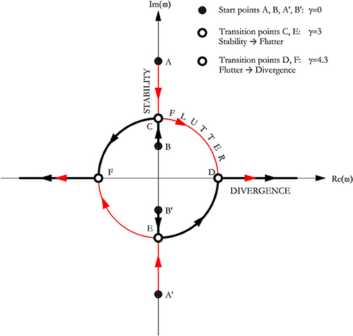
Figure 8. Codimension-one eigenvalues evolution of undamped Ziegler double pendulum under increasing follower load F (ρ = ℓ = k = c = 1) and v = 0.

FIGURE 9

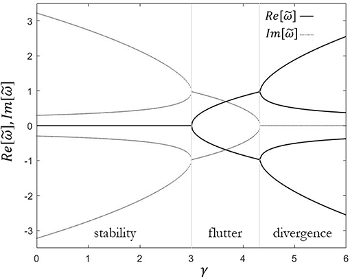
Figure 9. Real (solid line) and imaginary (dot line) parts of the eigenvalues $\tilde{\omega }$ vs. dimensionless follower load γ, for v = 0.

FIGURE 10

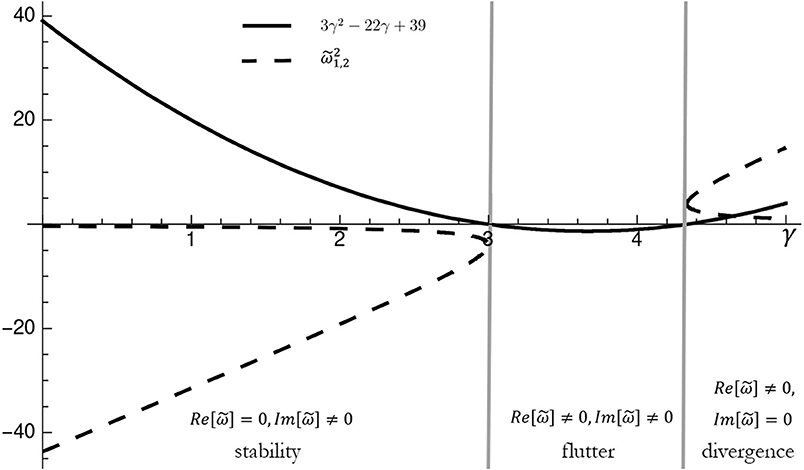
Figure 10. Graphical study of Equation (11) to identify the region of stability, for v = 0.

In the case of the viscoelastic Ziegler pendulum, for a suitably small value of ν, the critical load is smallest in the undamped case

$\begin{array}{ll}{P}_f=\left(\frac{4}{3}+\frac{{\nu }^2}{2}\right)\frac{k}{\ell }& (13)\end{array}$

As sketched in Figure 11, if we assume ν = 0.1 we obtain γ = 1.78 vs. γ = 3 of the undamped system. This is the well-known destabilizing effect of damping. The paradox is even more evident when we reduce the viscosity to zero (ν → 0), because the flutter load is still noticeably lower than those of the undamped system.

FIGURE 11

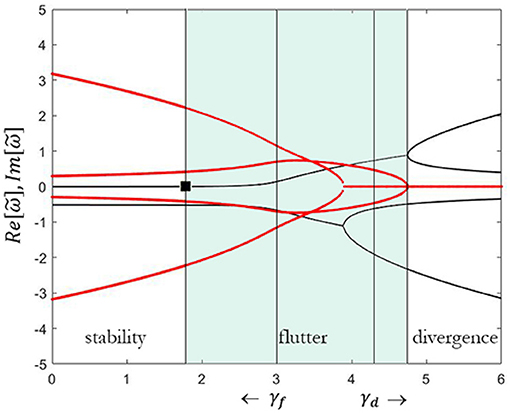
Figure 11. Real (black line) and imaginary (red line) part of the eigenvalues $\tilde{\omega }$ vs. dimensionless follower load γ, for ν = 0.1.

7. Experimental Investigations

The first experimental evidence of non-linear oscillatory behavior in mechanical systems dates to the 1660s and the pioneering works on pendulum dynamics by Marin Mersenne and Christiaan Huygen. Further experimental campaigns were conducted in the 1800s in an industrial context. Their aim was to recognize the flutter instabilities of the throttle valves of steam engines, the hunting motions of railway cars, the whirling of rotors and so on. In 1859, Franz Melde carried out an experiment on standing waves produced in a string made to oscillate via a tuning fork, which opened the way to new and fascinating knowledge in the field of parametrically excited vibrations. Thereafter, the experimental observation of dynamic instabilities saw a renewed interest in the 1970s, when researchers focused their efforts on the possibilities of dynamic bifurcations (saddle-node, pitchfork, period-doubling, and Hopf bifurcations) and on the routes to chaos and strange attractors (e.g., period-doubling cascades, torus breakdown, dynamic codimension-2 bifurcations etc.). In recent decades, a great amount of effort has been put into the study and experimental investigation of the dynamic snap-through of shallow arches and the local buckling of axially compressed shells under dynamic perturbation (see [61, 72] and references therein). Unlike their theoretical counterparts, however, experimental developments in the dynamic bifurcation of structures are still not well established, and a great deal of research remains to be done. This is most likely due to the difficulties entailed in the extreme sensitivity of the structural responses and, in certain cases, the practical difficulties related to analyzing mechanical models (this is the case for systems involving follower forces). For example, considerable work still needs to be done to close the gaps between theoretical and experimental studies on large-amplitude vibrations and the chaotic behavior of shells, plates and membranes (see [73] and references therein). The same can be said of the dynamic instability induced by follower forces (i.e., flutter and divergence). The difficulty, in these cases, is in practically realizing a tangential force [41]. This issue is still quite controversial. Certain researchers consider follower forces as a completely unrealistic “thought experiment,” undeserving of scientific consideration. Others, conversely, maintain that follower forces is a realistic topic with important real-world consequences. In this regard, two articles entitled “Unrealistic Follower Forces” and “Realistic Follower Force” by Koiter [74] and Sugiyama et al. [75], respectively, are an interesting contribution to both sides of the debate. Koiter, for his part, stresses:

The abundant literature on such non-conservative follower forces in the second half of the present century is devoid of any mechanism by means of which experiments on follower forces can be performed. The absence of such physical evidence reduces the concept of follower forces to a “Gedankenexperiment” without consequences in the real world.

A few years later, Sugiyama retorts:

Admiringly, even now, there is a group of scientists who do not believe in the reality of tangential follower forces. The origin of a follower force can be found in an end rocket thrust applied to flexible missiles and spacecraft. In this sense a follower force is a very realistic force in the field of aerospace structures engineering.

Bolotin [1] also spoke on the issue in 1999 as follows:

I am not at all a partisan of follower forces. It seems that since 1961 when I had published my book, I never returned to the topic. But one must be just: follower forces do exist, at least as a first approximation, as the models of real forces, such as jet responses and jet pressures. […] Actually, most of the publications on follower forces are of purely academic origin and seem artificial. […] Who knows, maybe we will meet this kind of problem in the future when dealing with smart space structures. But bluntly speaking, most recent papers on follower forces do not arouse much sympathy from me.

For more details on this controversy, see Elishakoff' enlightening overview [76] in which he underlines the need to deploy a large experimental campaign that can provide definite answers to the feasibility of follower forces. Recent experimentations performed by Bigoni and Noselli [77] and Bigoni et al. [78] are also very impressive. Not only do they confirm the feasibility of follower forces but their experimental results align qualitatively with their theoretical equivalents. However, Kurnik et al. [79] show that the system tested by Bigoni and Noselli [77] did not rigorously model the original Ziegler column. We can thus conclude that this issue is far from settled, and that further research will be required.

8. Next-Generation Challenges

Over the last decades, the dynamic stability of elastic structures have gone through a revival of interest across different application areas, due to the possibility to harness mechanical instabilities for additional functionality. Addressing the stability problem in terms of an opportunity to exploit (buckliphilia) rather than of catastrophe to avoid (buckliphobia) offers a new stimulating layer of depth to the issue. A case in point are the next-generation micro- or nano-electro-mechanical systems (MEMS or NEMS), which are becoming increasingly attractive to the scientific community due to their great potential and functional advantages, including their extended working range, tunable resonant frequencies, reliability, reconfigurability and cost-effectiveness [19, 80]. These bi-stable systems exhibit non-linear behaviors (softening or stiffening response, dynamic pull-in or snap-through, chaotic vibrations) that are tunable, for example, by prestress. They often exploit non-linearities (due to resonance, buckling, dissipation and electrostatic or piezoelettric actuation, to cite a few examples) as a means to increase their performance. On this point, the use of parametric resonance in MEMS is of particular applied interest as it leads to an interesting and rather unusual mixed softening-stiffening response. A considerable number of MEMS or NEMS devices uses a dynamic operating mode. Of particular interest to researchers are devices that exploit dynamic snap-through instability as an actuation mechanism or for filtering applications (e.g., band-pass filters). The range of applications is wide and varied: relays, switches, valves, mechanical memories, drive mechanisms (such as micro/nano-actuators), pressure sensors, varactors, inductors, resonetors, transducers, clips, threshold, controllers for micro-mirrors, etc. Numerous recent studies show how the dynamic snap-through instability of MEMS and NEMS shallow arches can be profitably employed; for example, for filter and switch applications.

A further leading area of research in the fields of structural health monitoring and non-destructive evaluation focuses on post-buckling-based energy harvesting devices, such as self-powered wireless sensors and sensor network [81]. Such devices exploit the post-buckling snap-through behavior to convert low-rate and low-frequency excitations into high-rate motions. The latter in turn can be employed to generate electric energy (by using, for example, piezoelectric transducers). This solves the major drawback of the traditional wireless sensors, that is the limited lifespan of batteries. Other appealing applications involve the use of limit cycles, self-sustained oscillation, and bifurcations for signal processing. Devices such as these, and especially bifurcation amplifiers, exploit the sudden transition (or “jump”) across bifurcations to amplify signals making them suitable for taking highly sensitive measurements.

The high-rate motion and multistability are appealing features of buckling phenomena which can usefully exploited at different scales for smart morphable or shape-adaptive structures, devices or metamaterials (inspired, for example, by origami or kirigami technique) [82]. This can be achieved by specific design strategies (e.g., the modal nurging) which lead the structure to a peculiar equilibrium path [83]. The periodic buckling, for example, can be usefully exploited to generate reversible or irreversible (depending on the type of material to be handled: shape-changing or shape-memory materials) transformations in topology. Specific examples of applications including self-deployable or -lockable structures, encapsulation devices, radiofrequency switchable components, transformable metamaterial structures, and many others.

9. Concluding Remarks

This paper set itself the ambitious goal of reviewing the recent literature on the fascinating topic of the linear and nonlinear dynamic instability of elastic mechanical systems. The aim was to identify and examine the priority areas for existing research, as well as those of significant future interest. The stability theory of dynamic systems is a captivating but complex issue, which incorporates many scientific disciplines. For this reason, it has been widely investigated over the last century and remains a highly active field of research. The more relevant and innovative works over the last two decades were considered here. However, given the volume of other similar research, others were inevitably omitted, and the author requests some indulgence on this point. Most of the key topics relating to dynamic instabilities are currently well-understood and mature. They have been adequately and extensively studied, both analytically and numerically. A lot has been done, for example, with regard to the exploitation of codimension-2 bifurcations; for example, snap-through as an actuation mechanism and for filtering applications (e.g., band-pass filters) in the tailorable design of arch-shaped micro/nano electromechanical system (MEMS/NEMS) devices and bi-stable curved nano-beams (nanotubes and nanowires). The exploitation of chaotic behavior and non-linear resonance in a variety of advanced engineering applications is a cutting-edge field in need of future attention from researchers. Two key examples are the impact dampers used in the passive control of vibrating systems, and the chaotic driven signal for system identification. The latter paves the way for urgently needed innovative tools to monitoring structures' state of health. Despite the available theoretical and numerical studies, experimental data on some complicated bifurcations, chaos and post-buckling behavior are much less frequent in the literature. This is especially true in the case of non-conservative systems under follower-forces, and of large-amplitude vibrations in panels and shells. In the cases of follower-forces, it remains a matter of debate as to whether they can be opportunely performed in an experimental setting. As such, this stands out as a rich source of future research.

Data Availability Statement

All datasets generated for this study are included in the manuscript.

Author Contributions

The author confirms being the sole contributor of this work and has approved it for publication.

Funding

IM gratefully acknowledges financial support from the Italian Ministry of Education, University and Research (MIUR) under the Departments of Excellence grant L.232/2016.

Conflict of Interest

The author declares that the research was conducted in the absence of any commercial or financial relationships that could be construed as a potential conflict of interest.

References

1. Bolotin VV. Dynamic instabilities in mechanics of structures. Appl Mech Rev. (1999) 40:R1–9. doi: 10.1080/15376494.2017.1410903

CrossRef Full Text | Google Scholar

2. Lyapunov AM. The general problem of stability of motion (in Russian) (Doctoral dissertation). University of Kharkov, Kharkiv, Ukraine (1892).

Google Scholar

3. Lindberg HE, Florence AL. Dynamic Pulse Buckling. Theory and Experiment. Dordrecht: Nijhoff Publishers (1987). doi: 10.1007/978-94-009-3657-7

CrossRef Full Text | Google Scholar

4. Simitses GJ. Dynamic Stability of Suddenly Loaded Structures. New York, NY: Springer-Verlag (1990). doi: 10.1007/978-1-4612-3244-5

CrossRef Full Text | Google Scholar

5. Seyranian AP, Elishakoff I. Modern Problems of Structural Stability. New York, NY: SpringerWien (2012). doi: 10.1007/978-3-7091-2560-1

CrossRef Full Text | Google Scholar

6. Kirillov ON, Bigoni D. Dynamic Stability and Bifurcation in Nonconservative Mechanics. Cham: Springer (2018). doi: 10.1007/978-3-319-93722-9

CrossRef Full Text | Google Scholar

7. Golubitsky M, Schaeffer DG. Singularities and Groups in Bifurcation Theory. Vol. I. New York, NY: Springer-Verlag (1985). doi: 10.1007/978-1-4612-5034-0

CrossRef Full Text | Google Scholar

8. Golubitsky M, Stewart I, Schaeffer D. Singularities and Groups in Bifurcation Theory. Vol. II New York, NY: Springer-Verlag (1988). doi: 10.1007/978-1-4612-4574-2

CrossRef Full Text | Google Scholar

9. Thomsen JMT. Vibrations and Stability, Advance Theory, Analysis and Tools. 2nd Edn. Verlang: Springer (2003).

Google Scholar

10. Kuznetsov YA. Elements of Applied Bifurcation Theory. 3rd Edn. New York, NY: Springer-Verlag (2010).

Google Scholar

11. Sugiyama Y, Langthjem MA, Katayama K. Dynamic Stability of Columns Under Nonconservative Forces: Theory and Experiment. Cham: Springer (2018).

Google Scholar

12. Simitses GJ. Instability of dynamically-loaded structures. Appl Mech Rev. (1987) 52:1403–8. doi: 10.1115/1.3149542

CrossRef Full Text | Google Scholar

13. Bolotin VV. The Dynamic Stability of Elastic System. San Francisco, CA: Holden-Day, Inc. (1964).

Google Scholar

14. Nayfeh AH, Mook DT. Nonlinear Oscillations. New York, NY: John Wiley and Sons (1979).

Google Scholar

15. Fossen TI, Nijmeije H. Parametric Resonance in Dynamical Systems. New York, NY: Springer-Verlag (2012). doi: 10.1007/978-1-4614-1043-0

CrossRef Full Text | Google Scholar

16. Seyranian AP. The swing: parametric resonance. J Appl Math Mech. (2004) 68:757–64. doi: 10.1016/j.jappmathmech.2004.09.011

CrossRef Full Text | Google Scholar

17. Paidoussis MP. Chapter 4: Pipes conveying fluid: linear dynamics II. In: Fluid-Structure Interactions, 2nd Edn. Slender Structures and Axial Flow (2014) Montreal, QC: Academic Press; Elsevier. p. 235–332. doi: 10.1016/B978-0-12-397312-2.00004-1

CrossRef Full Text | Google Scholar

18. Paidoussis MP. Chapter 2: Cylinders in axial flow I. In: Fluid-Structure Interactions, 2nd Edn. Slender Structures and Axial Flow (2016) Montreal, QC: Academic Press; Elsevier. p. 143–302. doi: 10.1016/B978-0-12-397333-7.00002-4

CrossRef Full Text | Google Scholar

19. Moran K, Burgner C, Shaw S, Turner K. A review of parametric resonance in microelectromechanical systems. Nonlinear Theory Appl. (2013). 4:198–224. doi: 10.1587/nolta.4.198

CrossRef Full Text | Google Scholar

20. Hoff NJ, Bruce VG. Dynamic analysis of the buckling of laterally loaded flat arches. J Math Phys. (1954) 32:276–88.

Google Scholar

21. Budiansky B, Roth RS. Axisymmetric dynamic buckling of clamped shallow spherical shells. In: Collected Papers on Instability of Shell Structures, NASA TN D-1510. Hampton, VA (1962). p. 597–606.

Google Scholar

22. Simitses GJ. Dynamic snap-through buckling of low arches and shallow spherical caps (PhD dissertation). Dept. of Aeronautics and Astronautics, Stanford University, Stanford, CA, United States (1965). doi: 10.2514/6.1966-1712

CrossRef Full Text | Google Scholar

23. Hsu CS. On dynamic stability of elastic bodies with prescribed initial conditions. Int J Eng Sci. (1966) 4:1–21. doi: 10.1016/0020-7225(66)90026-7

CrossRef Full Text | Google Scholar

24. Hsu CS. The effects of various parameters on the dynamic stability of a shallow arch. J Appl Mech. (1967) 34:349–58. doi: 10.1115/1.3607689

CrossRef Full Text | Google Scholar

25. Hsu CS. Stability of shallow arches against snap-through under timewise step loads. J Appl Mech. (1968) 35:31–9. doi: 10.1115/1.3601170

CrossRef Full Text | Google Scholar

26. Ziegler H. Die stabilitätskriterien der elastomechanik. Arch Appl Mech. (1952) 20:49–56. doi: 10.1007/BF00536796

CrossRef Full Text | Google Scholar

27. Ziegler H. Principles of Structural Stability. Basel; Stuttgart: Birkhäuser Verlag (1977).

Google Scholar

28. Crandall SH. The physical nature of rotor instability mechanisms. In: Adams ML, editor. Rotor Dynamical Instability. New York, NY: ASME; AMD (1983). p. 1–18.

Google Scholar

29. Krasovskii NN. Stability of Motion. Applications of Lyapunov's Second Method to Differential Systems and Equations With Delay. Translated by Brenner, J.L. Standford: Stanford University Press (1963).

Google Scholar

30. Thompson JMT, Hunt GW. A General Theory of Elastic Stability. London: John Wiley & Sons (1978).

Google Scholar

31. Török JS. Analytical Mechanics With an Introduction to Dynamical Systems. New York, NY: John Wiley & Sons, Inc. (2000).

Google Scholar

32. Obodan NI, Lebedeyev OG, Gromov VA. Nonlinear Behaviour and Stability of Thin-Walled Shells. New York, NY: Springer (2013). doi: 10.1007/978-94-007-6365-4

CrossRef Full Text | Google Scholar

33. Obodan NI, Gromov VA. The complete bifurcation structure of nonlinear boundary problem for cylindrical panel subjected to uniform external pressure. Thin-Walled Struct. (2016) 107:612–9. doi: 10.1016/j.tws.2016.07.020

CrossRef Full Text | Google Scholar

34. Groh R, Pirrera A. Exploring islands of stability in the design space of cylindrical shell structures. In: Pietraszkiewicz W, Witkowski W, editors. Proceedings of the 11th International Conference "Shell Structures: Theory and Applications, (SSTA 2017). Gdansk (2017). p. 223–6.

Google Scholar

35. Thompson JMT, Stewart HB. Nonlinear Dynamics and Chaos. 2nd Edn. Chichester: Wiley (2002).

Google Scholar

36. Awrejcewicz J, Krysko VA. Chaos in Structural Mechanics. New York, NY: Springer (2008). doi: 10.1007/978-3-540-77676-5

CrossRef Full Text | Google Scholar

37. Pugno N, Surace C, Ruotolo R. Evaluation of the non-linear dynamic response to harmonic excitation of a beam with several breathing cracks. J Sound Vib. (2000) 235:749–62. doi: 10.1006/jsvi.2000.2980

CrossRef Full Text | Google Scholar

38. Strogatz SH. Non Linear Dynamics and Chaos. With Applications to Physics, Biology, Chemistry, and Engineering. 2nd Edn. Reading, PA: Addison-Wesley Publishing Company (2015). doi: 10.1201/9780429492563

CrossRef Full Text | Google Scholar

39. El Naschie MS. Stress, Stability, and Chaos in Structural Engineering: An Energy Approach. London: McGraw-Hill (1990).

Google Scholar

40. Beck MS. Die Knicklast des einseitig eingespannten, tangential gedrück-ten Stabes. JAMP. (1952). 3:225. doi: 10.1007/BF02008828

CrossRef Full Text | Google Scholar

41. Bolotin VV. Nonconservative Problems of the Theory of Elastic Stability. New York, NY: Macmillan (1963).

Google Scholar

42. Nicolai EL. On stability of the straight form of equilibrium of a column under axial force and torque. Izv Leningr Politech Inst. (1928) 31:201–31.

Google Scholar

43. Guarracino F. Considerations on the numerical analysis of initial post-buckling behaviour in plates and beams. Thin-Walled Struct. (2007) 45:845–8. doi: 10.1016/j.tws.2007.08.004

CrossRef Full Text | Google Scholar

44. Guarracino F, Walker A. Some comments on the numerical analysis of plates and thin-walled structures. Thin-Walled Struct. (2008) 46:975–80. doi: 10.1016/j.tws.2008.01.034

CrossRef Full Text | Google Scholar

45. Obodan NI, Adlucky VJ, Gromov VA. Rapid identification of pre-buckling states: a case of cylindrical shell. Thin-Walled Struct. (2018) 124:449–57. doi: 10.1016/j.tws.2017.12.034

CrossRef Full Text | Google Scholar

46. Obodan NI, Adlucky VJ, Gromov VA. Prediction and control of buckling: the inverse bifurcation problems for von Karman equations. In: Dutta H, Peters JF, editors. Applied Mathematical Analysis: Theory, Methods, and Applications Studies in Systems, Decision and Control, Vol. 177. New York, NY: Springer (2019). p. 353–81. doi: 10.1007/978-3-319-99918-0_11

CrossRef Full Text | Google Scholar

47. Elishakoff I. A selected review of direct, semi-inverse and inverse eigenvalue problems for structures described by differential equations with variable coefficient. Achiev Comput Methods Eng. (2000). 7:451–526. doi: 10.1007/BF02736214

CrossRef Full Text | Google Scholar

48. Karnovsky IA. Theory of Arched Structures. Strength, Stability, Vibration. New York, NY: Springer (2011). doi: 10.1007/978-1-4614-0469-9

CrossRef Full Text | Google Scholar

49. Kam D, Chau T. Applications of Differential Equations in Engineering and Mechanics. 1st Edn. Boca Raton, FL: CRC Press (2018). doi: 10.1201/9780429470646

CrossRef Full Text | Google Scholar

50. Keskin AÜ. Adomian decomposition method (ADM). In: Boundary Value Problems for Engineers. Basel: Springer International Publishing (2019). p. 311–59. doi: 10.1007/978-3-030-21080-9_7

CrossRef Full Text | Google Scholar

51. Liao S, editor. Chapter 1: Chance and challenge: a brief review of the homotopy analysis method. In Advanced Homotopy Analysis Method. Shanghai: World Scientific Press (2013). p. 1–33. doi: 10.1142/9789814551250_0001

CrossRef Full Text | Google Scholar

52. Vladimir SI, Anatolu PV. Handbook of Mechanical Stability in Engineering. Sardar D, editor. Singapore: World Scientific (2013).

Google Scholar

53. Reddy JN. Energy Principles and Variational Methods in Applied Mechanics. 2nd Edn. New York, NY: John Wiley (2002).

Google Scholar

54. Guarracino F, Walker A. Energy Methods in Structural Mechanics: A Comprehensive Introduction to Matrix and Finite Element Methods of Analysis. London: Thomas Telford (1999).

Google Scholar

55. Simitses GJ, Hodges DH. Fundamentals of Structural Stability. Amsterdam: Elsevier (2006).

Google Scholar

56. Mallon NJ. Dynamic Stability of Thin-Walled Structures: A Semi-Analytical and Experimental Approach. Eindhoven: Technische Universiteit Eindhoven (2006). doi: 10.6100/IR637287

CrossRef Full Text | Google Scholar

57. Xie WC. Dynamic Stability of Structures. Cambridge: Cambridge University Press (2006).

Google Scholar

58. Keller HB. Numerical solution of bifurcation and nonlinear eigenvaue problems. In: Rabinowitz P, editor. Applications of Bifurcation Theory. New York, NY: Academic Press (1977). p. 359–84.

Google Scholar

59. Quarteroni A, Sacco S, Saleri F. Numerical Mathematics. Texts in Applied Mathematics. New York, NY: Springer (2010).

Google Scholar

60. Antia HM. Numerical Methods for Scientists and Engineers. New Delhi: Tata McGraw-Hill Publishing Company Limited (1991).

Google Scholar

61. Evkin A, Krasovsky V, Lykhachova O, Marchenko V. Local buckling of axially compressed cylindrical shells with different boundary conditions. Thin-walled Struct. (2019) 141:374–88. doi: 10.1016/j.tws.2019.04.039

CrossRef Full Text | Google Scholar

62. Bert CW, Malik M. Differential quadrature method in computational mechanics: a review. Appl Mech Rev. (1996) 49:1–28. doi: 10.1115/1.3101882

CrossRef Full Text | Google Scholar

63. Doedel EJ, Champneys AR, Fairgrieve TF, Kuznetsov YA, Oldeman B, Paffenroth RC, et al. AUTO-07p: Continuation and Bifurcation Software for Ordinary Differential Equations. Montreal, QC: Department of Computer Science; Concordia University (2007).

Google Scholar

64. Kuznetsov YA, Levitin VV. CONTENT: A Multiplatform Environment for Analyzing Dynamical Systems. Amsterdam: Dynamical Systems Laboratory; Centrum voor Wiskude en Informatica (1997).

Google Scholar

65. Dhooge A, Govaerts W, Kuznetsov YA. MATCONT: A MATLAB package for numerical bifurcation analysis of ODE's. ACM T Math Softw. (2003) 29:141–64. doi: 10.1145/980175.980184

CrossRef Full Text | Google Scholar

66. Godoy LA. Theory of Elastic Stability: Analysis and Sensitivity. Philadelphia, PA: Taylor and Francis (2000).

Google Scholar

67. Liang K. A Koiter-Newton arclength method for buckling-sensitive structures. (Ph.D. Thesis). Technische Universiteit Delft, Delft, Netherlands (2013). doi: 10.4233/uuid:19037c4d-d787-4cab-a182-6fcc33badf70

CrossRef Full Text | Google Scholar

68. Ford W. Chapter 18: The algebraic eigenvalue problem. In: Numerical Linear Algebra with Applications. London: Academic Press; Elsevier (2015). p. 379–438. doi: 10.1016/b978-0-12-394435-1.00018-1

CrossRef Full Text | Google Scholar

69. Peek R, Kheyrkhahan M. Postbuckling behavior and imperfection sensitivity of elastic structures by the Lyapunov-Schmidt-Koiter approach. Comput Method Appl Mech. (1993) 108:261–79. doi: 10.1016/0045-7825(93)90005-i

CrossRef Full Text | Google Scholar

70. Euler L. Determinatio onerum, quae columnae gestare valent. Acta Acad Sci Petropol. (1778) 1:121–45. doi: 10.2514/3.3561

CrossRef Full Text | Google Scholar

71. Kirillov ON, Verhulst F. Paradoxes of dissipation-induced destabilization or who opened Whitney's umbrella? J Appl Math Mech. (2010) 90:462–88. doi: 10.1002/zamm.200900315

CrossRef Full Text | Google Scholar

72. Virot E, Kreilos T, Schneider TM, Rubinstein SM. Stability landscape of shell buckling. Phis Rev Lett. (2017) 119:224101. doi: 10.1103/PhysRevLett.119.224101

PubMed Abstract | CrossRef Full Text | Google Scholar

73. Amabili M, Païdoussis MP. Review of studies on geometrically nonlinear vibrations and dynamics of circular cylindrical shells and panels, with and without fluid-structure interaction. Appl Mech Rev. (2003) 56:349–81. doi: 10.1115/1.1565084

CrossRef Full Text | Google Scholar

74. Koiter WT. Unrealistic follower forces. J Sound Vib. (1996) 194:636. doi: 10.1006/jsvi.1996.0383

CrossRef Full Text | Google Scholar

75. Sugiyama Y, Langthjem MA, Ryu BJ. Realistic follower forces. J Sound Vib. (1999) 225:779–82. doi: 10.1006/jsvi.1998.2290

CrossRef Full Text | Google Scholar

76. Elishakoff I. Controversy associated with the so-called “follower forces”: critical overview. Appl Mech Rev. (2005) 58:117–42. doi: 10.1115/1.1849170

CrossRef Full Text | Google Scholar

77. Bigoni D, Noselli G. Experimental evidence of flutter and divergence instabilities induced by dry friction. J Mech Phys Solids. (2011) 59:2208–26. doi: 10.1016/j.jmps.2011.05.007

CrossRef Full Text | Google Scholar

78. Bigoni D, Kirillov ON, Misseroni D, Noselli G, Tommasini M. Flutter and divergence instability in the Pflüger column: experimental evidence of the Ziegler destabilization paradox. J Mech Phys Solids. (2018) 116:99–116. doi: 10.1016/j.jmps.2018.03.024

CrossRef Full Text | Google Scholar

79. Kurnik W, Przybylowicz PM, Bogacz R. Bigoni and Noselli experiment: is it evidence for flutter in the Ziegler column? Arch Appl Mech. (2017) 88:203–13. doi: 10.1007/s00419-017-1294-1

CrossRef Full Text | Google Scholar

80. Senturia SD. Microsystem Design. Boston, MA: Springer US (2001). doi: 10.1007/b117574

CrossRef Full Text | Google Scholar

81. Reis PM. A perspective on the revival of structural (in)stability with novel opportunities for function: from buckliphobia to buckliphilia. J Appl Mech. (2015) 82:111001–1–1–4. doi: 10.1115/1.4031456

CrossRef Full Text | Google Scholar

82. Hu N, Burgueño R. Buckling-induced smart applications: recent advances and trends Smart Mater Struct. (2015) 24:063001. doi: 10.1088/0964-1726/24/6/063001

CrossRef Full Text | Google Scholar

83. Cox BS, Groh RMJ, Avitabile D, Pirrera A. Modal nudging in nonlinear elasticity: tailoring the elastic post-buckling behaviour of engineering structures. J Mech Phys Solids. (2018) 116:135–49. doi: 10.1016/j.jmps.2018.03.025

CrossRef Full Text | Google Scholar