 Alexandra Livada1*
 Maria Christina Anagnostopoulou2
- 1Department of Statistics, Athens University of Economics and Business, Athens, Greece
- 2Statistics Department, London School of Economics, London, United Kingdom
Introduction
Financial volatility, risk measures and inequality are issues that concern not only finance and economics. It is a rather broad topic related to politics, education, health, and many other areas in social sciences. The globalization and the economic crisis of 2008 have made volatility modeling one of the most attractive research topics [1]. On the other hand, income inequality is the main issue for the economic growth of any country. How do inequality, financial volatility and risk measures behave during the periods of economic crisis?
Academics and financial institutions develop sophisticated models in order to estimate and forecast volatility and market risk. Volatility, which is the main characteristic of any financial asset and its return, plays a very important role in many financial applications. Its primary role is to estimate the value of market risk. Well-known measures for the estimation-evaluation of market risk are Value-at-Risk (VaR) and Expected Shortfall (ES). Value-at-Risk is referring to a “portfolio's worst outcome which is likely to occur at a given confidence level” while Expected Shortfall is “the average of all losses which are greater or equal than Value-at-Risk.” The family of ARCH-GARCH models is the main representative of the parametric models used for the calculation of Value-at-Risk and Expected Shortfall measures.
Though volatility in financial data is not directly observable, it has some characteristics commonly seen in asset returns. These characteristics, known as “stylized facts” of financial time series returns, are mainly summarized to the volatility clustering [2] and leverage effect [3], along with a distribution which is heavy-tailed with downward skew and strong autocorrelations in squared returns. The Generalized Autoregressive Conditional Heteroskedasticity (GARCH) model and its extensions are able to capture volatility clustering very efficiently. This is known in the literature as Univariate ARCH-GARCH modeling. One the other hand, there are many ways to observe and measure income inequality. One of the most popular measures of income inequality is the examination of top income shares, which gives important indications of the structure of long-term economic development [4].
On the other hand, there is important voluminous recent literature developed, especially after the 2008 crisis [5–7] on how much volatility contributes to inequality.
The target of this paper is to present the inequality evolution through the evolution of the top 1%'s income share and at the same time try to connect and compare the performance of alternative ARCH/GARCH univariate models for the estimation of 95%Value-at-Risk (VaR) and 95%Expected Shortfall (ES) measures for three equity indices. We draw conclusions about which methods fit better according to certain statistical criteria. We implement six alternative specifications of ARCH-GARCH family volatility models—GARCH(1,1), GARCH(1,2), GARCH(2,1), EGARCH(1,1), TGARCH(1,1), GJR GARCH(1,1)—under two distributional assumptions, the normal error and Student-t distributions. The alternative distributions allow selecting a more flexible model for the return tails. For this purpose, daily data of three stock exchange indices have been used. The financial time series data used are the US S&P500, the British FTSE 100 and the German DAX. The period studied is from January 2000 to May 2015. The criteria for the period chosen is the availability of inequality data. The criteria for the country choice are mainly inequality data availability from the same data bank for the same period of time. Specific R code packages (urgarch, mrgarch, Performance Analytics) have been used for the estimation. The VaR one-day-ahead out-of-sample forecasts are evaluated according to Kupiec's and Christoffersen's tests. ES is evaluated through the estimation of Loss Function.
This paper is structured as follows: Firstly, we discuss briefly the financial data employed as well as inequality data. Then, in section Estimation of GARCH Models, we present the estimated coefficients of the univariate GARCH models, which are GARCH, EGARCH, TGARCH, and GJR-GARCH under two alternative error distributions. Next, volatility forecasts and 95%VaR as well as 95%ES estimates produced by alternative GARCH models are shown. Evaluation of various GARCH models' average 95%VaR and 95%ES estimates based on Kupiec's and Christoffersen's criteria and respective Loss Function are also discussed. Finally, conclusions are presented in section Conclusions, as well as possible future research extensions.
Data and Stylized Facts
For our study, we use daily data from three stock indexes: the Chicago Standard and Poor's 500 (S&P500), the London Financial Times Stock Exchange 100 (FTSE100) as well as the German Stock Index (DAX30). The data cover the period January 2000-May 2015. For all three indices, the evolution of their adjusted closing prices and their continuously compounded daily returns are illustrated in Figures 1, 2, respectively.
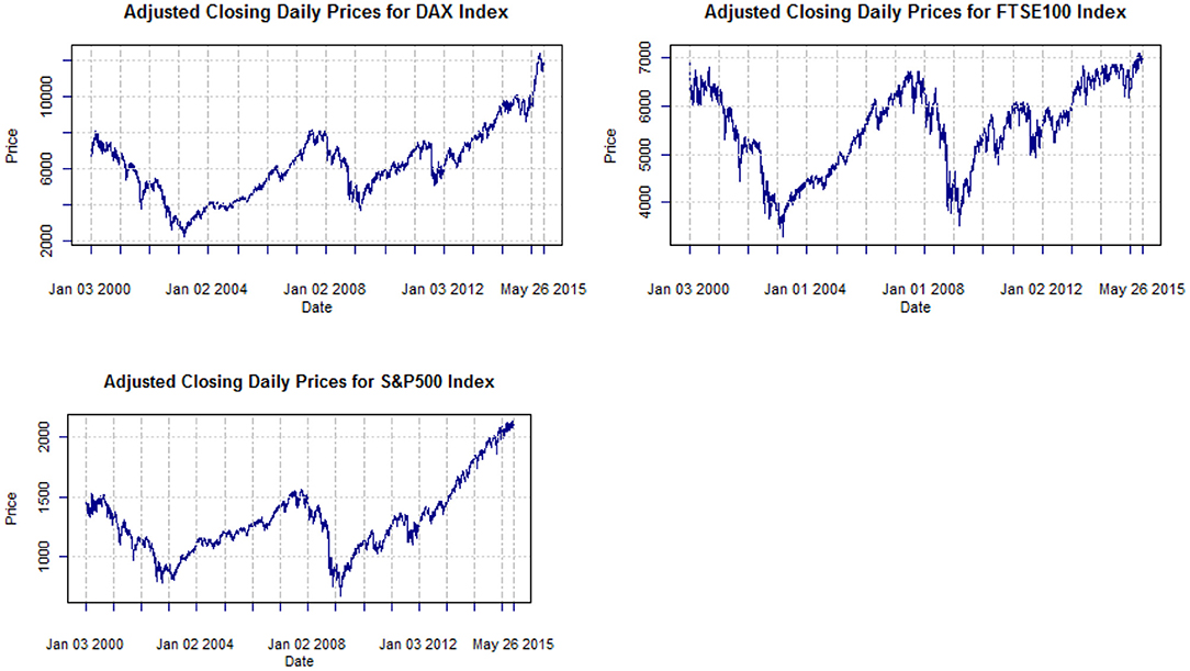
Figure 1. Adjusted closing prices of DAX, FTSE100, and S&P500 from Jan. 2000 to May 2015.
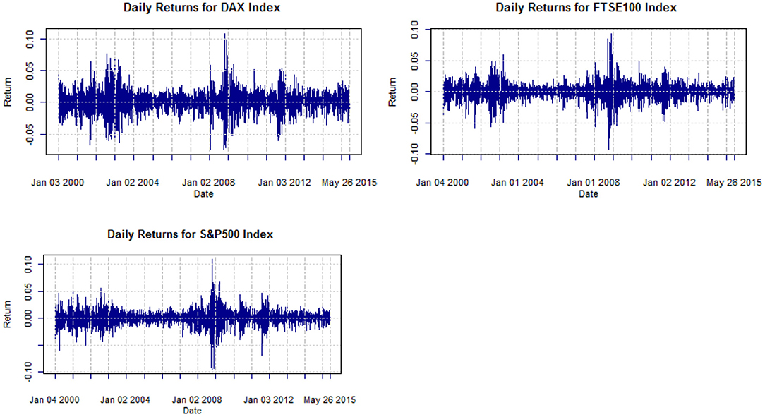
Figure 2. Daily returns of adjusted closing prices of DAX, FTSE100, S&P500, from Jan. 2000 to May 2015.
The most important financial events that are responsible for the main financial crises, depicted in Figure 1, are the following: In 2000, a massive fall in equity markets from over-speculation in tech stocks was produced by dot-com bubble pops. After that, in 2001, another junk bond crisis took place and the crisis in Argentina resulted in defaulting payment obligations by the government. Also, the September 11th attacks of the same year hindered various critical communication hubs creating great risk. The next year, 2002, a serious bond market crisis in Brazil took place. Five years later, in 2007 US real estate resulted in the collapse of massive international banks and financial institutions. In September 2008, Lehman Bros. bankruptcy takes place, creating a great fall and in the 29th of the same month the Dow Jones falls 778 points. In February of 2009, the Financial Stability Plan is announced and the Recovery Act is signed. This global crisis did not start at the same time for every country, for instance the U.K officially enters recession in January 2009.
Visual inspection of indices in Figure 2 shows clearly that the mean is constant, but the variance keeps changing over time, so the return series does not appear to be a sequence of i.i.d. random variables. The stylized fact noticeable from the figures is the volatility clustering according to Madelbrot [2] and Famma [8]. Table 1 provides summary statistics as well as Jarque-Bera statistic for testing normality. In all cases, the null hypothesis of normality is rejected and there is evidence of excess kurtosis and asymmetry.
Table 1. Summary statistics of the S&P500, FTSE100, DAX equity indices (ln- returns).
In Figure 3, we may observe the phenomenon of leverage by plotting the daily market prices and their volatility (standard deviations of the continuously compounded returns). The periods of market drops are followed by a large increase in volatility. The leverage effect is captured by asymmetric conditional volatility specification models presented in sections below.
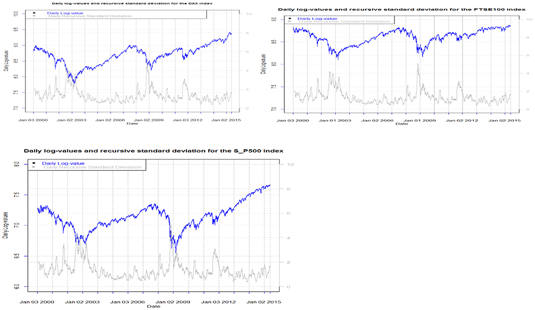
Figure 3. Daily logvalues and recursive standard deviation of returns for all indices.
Inequality Evolution: 1% Top Income Shares in USA, UK, Greece and France
One of the most popular measures of income inequality is the examination of top income shares [9] which gives important indications of the structure of long-term economic development [4]. In this section we discuss the 1% top income share using a set of macroeconomic factors for the period 1971–2014. We tested [10] for the existence of a long-run relationship between 1% top income share (tis) and the other macroeconomic factors for the cases of France, UK, Greece and USA [11] using the bounds test for cointegration proposed by Pesaran et al. [12].
According to the current literature on income inequality, we utilize tax data for the period 1972–2014 in order to study top income shares, following the suggests [13] methodology.
More specifically, we investigated [10] how and to what extent the main macroeconomic factors may affect income inequality as measured by top income shares. The macroeconomic indicators of most interest are the economic development and the openness of the economy, as well as education, financial development, and inflation.
The methodology of Autoregressive Distributed Lag (ARDL) cointegration is employed to analyze empirically the long-running relationships and dynamic interaction among the variables of interest. The findings refer to the period before and after the economic crisis for USA, UK, Greece and France. If the results are favorable, we can continue forming the long-run relationship, calculating the long-run multipliers, the short-run dynamics, the speed of the adjustment to the long-run equilibrium, etc. If the results show no signs of cointegration among the variables, the formation of the long-run relationship and those that were described above would be meaningless because the results would be spurious.
For the cases of France and Greece the ARDL test concluded in favor of the existance of a long-run relationship. In the case of USA the unit root tests shows that tis01 is trend stationary but it is a generate one while for UK the test is incocnclusive so we are not able to suggest a long run relationship [10]. In Table 2, we present some summary statistics about the tis01 series for each country. The results in the table are calculated using the data for the period 1971 to 2014. The evolution of income inequality as this is captured from the 1% top income shares and the respective yearly changes are presented in Figures 4, 5. We notice that there is a sharp upward increase of the 1%tis after the mid 80s' period for all three countries. The 2008-09 economic crisis is captured with a violent decrease in France and UK but not for the USA. So, the financial implications of the 2008 economic crisis affected some countries more heavily than others.
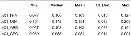
Table 2. 1% Top income share: summary statistics.
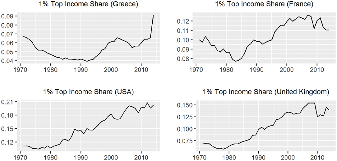
Figure 4. The evolution of 1% top income shares.
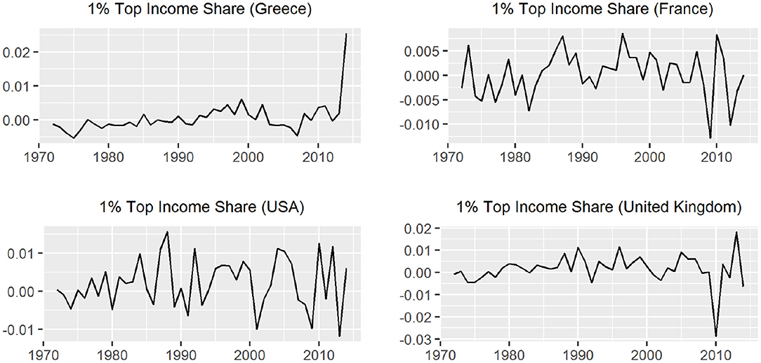
Figure 5. The evolution of first differences of the 1% top income shares.
So, if we study carefully Figures 2–5 we notice that the deep recession in the stock market in 2008 does not affect immediately the 1% top income share. The inequality effect is not the same in all four countries with respect to time, duration, and sharpness. That is, in Greece the consequences came almost immediately with sharper changes in the inequality index than other countries. There is also a long-lasting period of continuously rising inequality [14]. On the other hand, in USA, UK, and France the effect of the crisis shows a decline in the 1% top income share, which appears later (after 2010) but is not that sharp as in Greece (in mean levels) and shows mixed year to year changes. The trend in USA seems to be unaffected while in UK and France there is a slight trend change, which signals trend ambiguity.
But what if we try to connect these findings with the risk measures? Which model should we use in order to connect volatility with risk measures and then to inequality?
In the following section an econometric analysis is applied in order to choose the best fitting model to volatility data.
Estimation of GARCH Models
In this section, we present and discuss for all three equity indices the estimation of three symmetric GARCH(p,q) models and three asymmetric GARCH(1,1) under two error distributions: the Normal and Student-t. The respective estimated specifications are as follows: GARCH(1,1), GARCH(1,2), GARCH(2,1), EGARCH(1,1), TGARCH(1,1), and GJR-GARCH(1,1). For the estimation of these models, we used the fGARCH package, which follows model specification (2.11), as well as Performance Analytics and ugarch. For all models, the AIC [15] and SBC criteria are presented in Table 3. For each equity index, the best symmetric GARCH(p,q) is selected according to the best SBC criterion. All three asymmetric models for each index are also presented analytically in Tables 4–6 under two error distributions: the normal and student-t. For all considered models, tests are conducted for their residuals for autocorrelation (Ljung and Box's Q-test) and for heteroscedasticity (ARCH LM tests). Almost all models do not violate the homoskedasticity hypothesis. In Table 7 the findings are as follows:
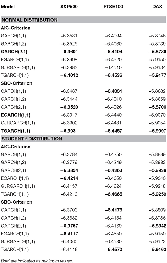
Table 3. Values of SBC and AIC criteria for all models.
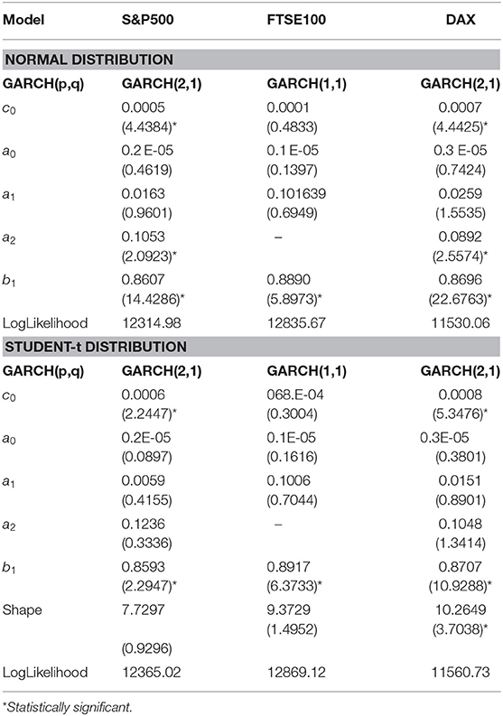
Table 4. Parameter estimates of symmetric GARCH(p,q) models for three equity indices using the entire data set and assuming two alternative distributions for the residuals, t-statistics are presented in parentheses.
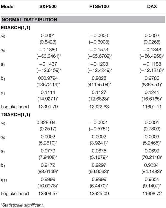
Table 5. Parameter estimates of EGARCH and TGARCH models for three equity indices using the entire data set and assuming normal distribution for the residuals, t-statistics are presented in parentheses.
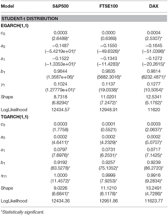
Table 6. Parameter estimates of EGARCH and TGARCH models for three equity indices using the entire data set and assuming Student-t distribution for the residuals, t-statistics are presented in parentheses.
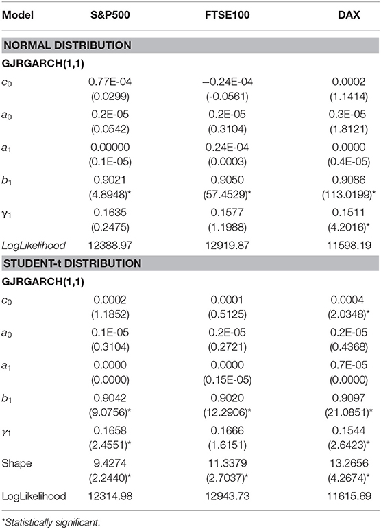
Table 7. Parameter estimates GJRGARCH model for three equity indices using the entire data set and assuming two alternative distributions for the residuals, t-statistics are presented in parentheses.
For the symmetric GARCH models for all equity indices for both error distributions, the best model according to both AIC and SBC criteria is GARCH(2,1), with the only exception of FTSE, where GARCH(1,1) is suggested by SBC.
For the asymmetric GARCH models, under the normal distribution for the indices S&P500, DAX, and FTSE, both AIC and SBC criteria suggest that TGARCH(1,1) is the best.
Under the Student-t: For both AIC and SBC the TGARCH(1,1) is the best for FTSE and DAX indices. EGARCH(1,1) is the best for S&P500.
In Table 4, where the estimated parameters of best symmetric GARCH models are presented, we notice that the conditional variance parameters are highly significant and that the distribution of zt has significantly thicker tails than the normal. In Tables 5, 6, where the estimated parameters of the asymmetric EGARCH(1,1) and TGARCH(1,1) specifications are presented, we notice that all coefficients are statistically significant under both distributions. The leverage effect is present in all EGARCH(1,1) and TGARCH(1,1) models for all indices since the respective coefficients are significantly different from zero. The GJR presented in Table 7 for both distributions does not capture the overall volatility equally well for all indices as by EGARCH(1,1) and TGARCH. In all tables, the reported t-statistics are estimated from robust standard errors.
Value-at-Risk and Expected Shortfall
Value-at-Risk (VaR) reports, for a given portfolio, the financial risk which refers to the worst outcome that may occur over a certain period and at a certain confidence interval. An extended discussion for VaR can be found in Best [16] and Dowd [17] as well as in Bauwens et al. [18]. There are also many references on VaR application (see [19–21]).
However, there are criticisms for VaR that the underlying statistical assumptions are violated [22–25], while [26] argued that alternative risks for management techniques produce different VaR forecasts, and this might affect the accuracy of risk estimate. Moreover, Marshall and Siegel [27] proved that if we consider the same portfolios, we may find statistically significant differences, while according to Artzner et al. [28, 29], VaR is not necessarily sub-additive for the case of more than one instruments. In order to overcome VaR shortcomings, Artzner et al. [28] introduced the Expected Shortfall (ES) risk measure, which estimates the expected value of loss in the case of a VaR violation. In this paper, both VaR and ES are estimated.
VaR, at a given probability level (1 − p), is defined [30–32] as the predicted amount of financial loss of a portfolio over a given time horizon. IfPt is the observed value of a portfolio at time t, and is the ln-returns for the period from t − 1 to t, then for a long trading position and under the assumption of standard normally distributed ln-returns, VaR is defined to be the value satisfying the condition below:
This implies that
where ζp is the (100p)-th percentile of the standard normal distribution.
So, under the assumption that yt ~ N(0, 1), the probability of a loss less than is equal to p = 5%.
Value-at-Risk is estimated via the parametric approach through the ARCH-GARCH framework below.
Suppose that the ln-returns yt can be expressed by
where μt is the expected return of portfolio for the period from t − 1 to t, and εt is the error term. The unpredictable part of the ln-returns is expressed with an ARCH process as presented in section Data and Stylized facts, that is:
where, as usual, zt denotes a random variable with density function f(0, 1;w), with mean equal to zero and variance equal to one, and w is a parameter vector to be estimated. The VaR value in this case is given by
where fa(zt; w) is the a-quantile of the assumed distribution, computed on the basis of the information set available at time t, and μt+1|t and σt+1|t are respectively the conditional mean and conditional standard deviation forecasts at time t+1 given the information at time-t. The one-step-ahead VaR forecast, based on ARCH model, is given by
Expected Shortfall (ES) provides information about the expected loss in the case of an extreme event, summarizing the risk in just one number. It is a better risk measure since according to Yamai and Yoshiba [33] it is more reliable during market turmoil. ES is a probability weighted average of tail loss, and the one-step-ahead ES is defined mathematically as below:
In order to calculate ES, we may follow [17], who estimated VaR by slicing the tail into a large number of segments of equal probability mass. Then, VaR is associated with each segment and ES is calculated as the average of these VaR estimates as below:
Backtesting VaR
Financial institutions pay great attention to the accurate estimation of 95 or 99%VaR. In real life if VaR is overestimated it leads regulators to charge higher amount of capital than is really needed, and this has a negative impact on their performance. The risk that financial institutions face may not be covered by the regulatory capital left aside if VaR is underestimated. The most simple method for the accurate evaluation of VaR forecast is to count in how many cases the losses exceed the value of VaR. If this count is not substantially different from what is expected, then the VaR forecasts are sufficiently computed.
The most well-known statistical methods for evaluating VaR models are Kupiec's [34] and Christoffersen's [35, 36], which are back-testing measures. Inference of these methods focus on hypothesis testing about the percentages of times a portfolio loss has exceeded the estimated VaR.
Kupiec [34] introduced a back testing method in terms of a hypothesis test for the expected percentage of VaR violations and used the observed rate at which the portfolio loss has been violated by the estimation of VaR in order to test whether the real coverage percentage p* is statistically significantly different from the desired level p.
The tested hypotheses are as follows:
The likelihood ratio test under null hypothesis is as follows:
where is the period that loss is more than the estimated VaR. N is the number of trading days that follows a binomial distribution under H0 with parameters and p. LRun is asymptotically χ2 distributed with one degree of freedom. This test is known as unconditional covariance test. The null hypothesis is rejected for both a statistically significantly low and high failure rate.
Christoffersen [35] introduced a testing method based on the expected percentage of having a VaR violation event conditional on the number of times it occurred in the past in a first order Markov set up and tested whether VaR violation events are independent with each other or not. That is, he tested (11) for trading days:
Therefore, the probability of observing a violation in VaR in two serial periods must be equal to the desired p value. The hypotheses tested are:
The hypotheses were tested using a LRin likelihood ratio statistic that follows asymptotically the χ2 distribution with one degree of freedom:
Where is the sample estimate of πij and nij is the number of trading days with value i followed by j, for i,j = 0,1.
Christoffersen [35] also suggested to test simultaneously whether the true percentage p* of failures is equal to the desired percentage and whether the VaR failure process is independently distributed. So, the following hypotheses were tested
The LRcc follows χ2 distribution with two degrees of freedom:
Conditional coverage process rejects a model that gives either many or very few clustered violations.
Because VaR does not indicate the size of the expected loss, Degiannakis and Angelidis [37] introduced utilizing loss function that are based on ES.
When we compare alternative models, according to ES loss function we prefer the model that gives lowest total loss value. This is equal to the sum of the penalty scores, . In this study we estimate (17) augmented by one.
One-Day-ahead Value-at-Risk and Expected Shortfall Forecasting
In this section we estimate the one-day-ahead 95% VaR and 95% ES values for all three indices. For each equity index we apply a model with constant mean ARMA(0,0) and conditional variance as GARCH(1,1), GARCH(1,2), GARCH(2,1), EGARCH(1,1), TGARCH(1,1), and GJRGARCH(1,1) volatility specifications presented before, for daily ln-returns under two distributional assumptions (Normal and Student-t). For all equity indices and all above models we have estimated 95%VaR and 95% ES forecasts for 500 trading days based on a rolling sample. Tables 8–10 present, for each equity index and 12 volatility models, the average values for the one-day-ahead 95% VaR and 95% ES forecasts as these are defined in the previous section. We also report the percentage of violations expressed by the number of violations over the out-of-sample 500 forecasts (N/T), Kupiec's and Christoffersen's p-values and the average value of the Loss Function based on the Expected Shortfall augmented by the value of one. A high p-value is preferred since this means that a good model will not overestimate or underestimate the true VaR. This is important because a high VaR estimation implies an obligation to allocate more capital than is actually necessary.
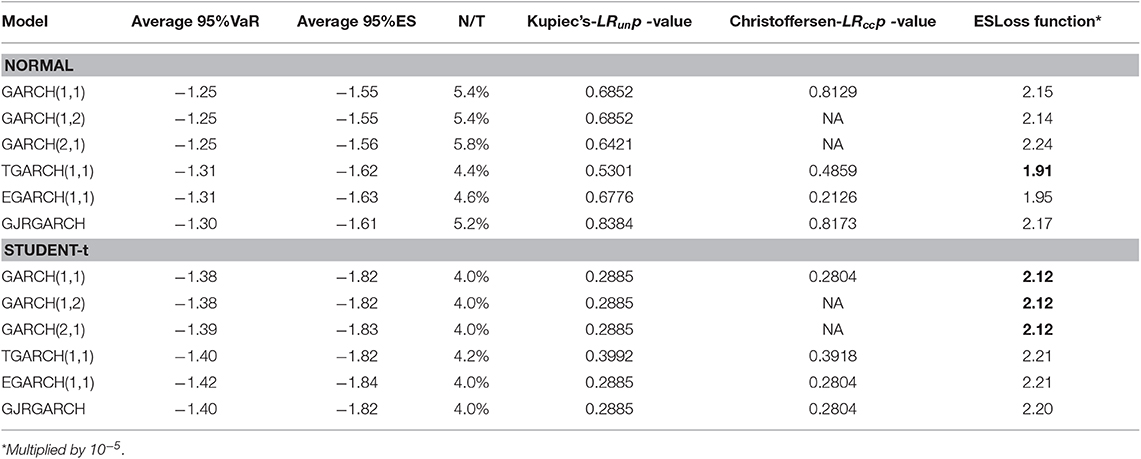
Table 8. FTSE equity index: 95%VaR and 95%ES average values of one-day-ahead forecasts, percentages of violation (N/T), Kupiec's and Christoffersen's p-values and ES loss function.
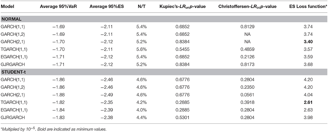
Table 9. DAX equity index: 95%VaR and 95%ES average values of one-day-ahead forecasts, percentages of violation (N/T), Kupiec's and Christoffersen's p-values and ES loss function.
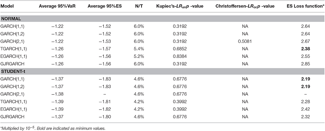
Table 10. S&P500 equity index: 95%VaR and 95%ES average values of one-day-ahead forecasts, percentages of violation (N/T), Kupiec's and Christoffersen's p-values and ES loss function.
For all equity indices we notice that the percentage of violations is greater for all indices and all model specifications under the assumption of normal distribution compared with that of Student-t. Thus, the Student-t gives less violations. However, we have to take into account firstly that the period forecasted is not very volatile and secondly the period of trading days we forecast may be considered small. In almost all cases, according to both Kupiec's and Christoffersen's test p-values reported in the Tables 8–10, we fail to reject the null hypothesis.
For the case of FTSE, for the normal distribution case the observed average 95%VaR gets values between (−1.31, −1.25) and for the Student-t distribution (−1.42, −1.38). The observed average 95% ES has values between (−1.6, −1.55) for the Normal distribution, which are larger (algebraically) compared to the values of Student-t distribution (−1.84, −1.82). The ES Loss function in the normal distribution has the lowest price for TGARCH(1,1) model (1.91), while in the Student-t case it has the lowest price in the three symmetric GARCH models (Equation 12). According to Kupiec's LRun p-value, the best model in normal distribution is the GJRGARCH(1,1), [38] with a p-value equal to 0.8384. In the Student-t distribution, all models have very low Kupiec's LRun p-values. For the cases where Christoffersen's p-values are available these are in agreement with Kupiec's.
Overall, our average 95%VaR one-day-ahead estimates based on univariate models suggest that all indices have the smaller score (larger in absolute values) under Student-t distribution.
According to Kupiec's LRun p-value, some models and indices share the highest p-values, for instance for normal distribution FTSE, and DAX has a p-value equal to 0.838 for the GJRGARCH(1,1). For the Student-t case, there is no common behavior regarding unconditional and conditional coverage tests, showing lower p-values than normal distribution in the majority of indices and respective models.
Because a greater p-value of the model does not indicate superiority, in order to evaluate the models, we computed Loss function based on ES. The score of the ES-Loss Function suggests as the best model the asymmetric TGARCH(1,1) model for most indices. For the Student-t case the ES loss function suggests for FTSE and S&P500 the GARCH(1,1), and for DAX the TGARCH(1,1).
So, we may conclude that in almost all cases the null hypothesis is not rejected. One of the reasons is the sample size, which in our case is a small one. This can be supported by Brooks and Persand [39] and Angelidis et al. [40], who argue that the effect of the sample size on the performance of the models is not clear.
In Figure 6, 95%VaR and 99%VaR one-day-ahead forecasts are visualized of all three indices studied. The VaR values are one-day-head, for 500 trading days. As expected, we have more violations for the 95%VaR than for the 99%VaR. So, risk measures capture adequately the volatility. We notice that business cycles are present in risk measures as in the inequality measures. At the beginning of 2014, there were low values of VaR and at the same time the top 1% share increases in 3 out of the 4 countries we study. However, the opposite holds for the period just before 2014. This could be an indication that risk measures are not closely related to income inequality. For a more accurate result we need more data and a business cycle study connecting risk measures with volatility and income inequality.
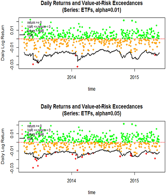
Figure 6. VaR exceedances and daily returns.
Conclusions
This paper is an attempt to combine financial volatility with income inequality and risk measures. It is an applied study where the evolution of income inequality is based on the top 1% income share for three European countries France, Greece, UK, and USA. These are countries with different levels of development, but all of them have homogenous time series inequality data. Most of the top income shares data are taken from the World Inequality Database. The financial risk measures are presented through the 95%VaR (Value-at-Risk) and ES(Expected shortfall) of three stock exchange indexes (S&P500, FTSE100, DAX30) which are based on ARCH/GARCH models. The financial volatility period covered is from 2000 to 2015.
We first study and compare the stylized facts of the Stock Exchange and inequality indices. Then, we compare the performance of a class of alternative univariate ARCH/GARCH models for the estimation of one-day ahead 95% Value-at-Risk (VaR) and Expected Shortfall (ES) measures for three equity indices. We implement six alternative specifications of ARCH-GARCH family volatility models: GARCH(1,1), GARCH(1,2), GARCH(2,1), EGARCH(1,1), TGARCH(1,1), GJR GARCH(1,1) under two distributional assumptions, the normal and Student-t distributions error. The alternative distributions allow for selecting a more flexible model for the return tails. The 95%VaR out of sample forecasts, for all models, are evaluated according to Kupiec's and Christoffersen's tests. ES is evaluated through the estimation of a Loss Function.
Regarding income inequality, we notice that there is an upward sharp increase of the 1% tis after the mid 80s period for all four countries. The 2008-09 economic crisis affected all countries. However, the deep recession in the stock market in 2008 did not affect immediately the 1% top income share. The inequality effect is not the same in all the four countries with respect time, duration and sharpness (see also [41]). The inequality effect is not the same in all the four countries with respect to time, duration and sharpness. That is, in Greece the consequences came almost immediately with sharper changes in the inequality index then other countries. There is also a long-lasting period of continuously rising inequality. On the other hand, in USA, UK, and France, the effect of the crisis shows a decline in the 1% top income share, which appears later (after 2010), but is not as sharp as in Greece (in mean levels) and shows a mixed year to year changes. The trend in USA seems to be unaffected while in UK and France there is a slight trend change, which signals trend ambiguity.
But what if we try to connect these findings with the risk measures? Which model should we use in order to connect volatility with risk measures and then to inequality?
The applied stochastic time series analysis for the financial indices of FTSE100, DAX30, S&P500 proves that the best models are under the Student-t distribution. More specifically, the TGARCH(1,1) model is the best for FTSE and DAX indices while for S&P500, the EGARCH(1,1) model fits better.
The 95%VaR and 95%ES forecasts show that for all model specifications of all equity indices, the percentage of violations is greater under the assumption of normal distribution compared with that of Student-t. We have to take into account that the forecasted period is not extremely volatile and that the period of trading days we forecast may be considered small. In almost all cases, tests of Kupiec's and Christoffersen's p-values fail to reject the null hypothesis.
Overall, our average 95%VaR one-day-ahead estimates based on univariate models suggest that all indices have the smaller value (larger in absolute values) under Student-t distribution.
According to Kupiec's LRun p-value, some models and indices share the highest p-values. For the Student-t case, there is no common behavior regarding unconditional and conditional coverage tests, showing lower p-values than normal distribution in the majority of indices and respective models. The score of the ES-Loss Function suggests the asymmetric TGARCH(1,1) as the best model in almost all indices under the normal distribution. For the Student-t case, the ES Loss Function suggested to be best for FTSE and S&P500 is the GARCH(1,1) model and for DAX it is the TGARCH(1,1) model.
VaR (95 and 99%) one-day-head for 500 trading days forecasts was visualized for all three indices studied, and as expected, we have more violations for the 95%VaR than for the 99%VaR. Risk measures used in this study capture adequately the volatility. We notice that business cycles are present in risk measures as in the inequality measures. At the beginning of 2014 there are low values of VaR and at the same time the top 1% share increases in 3 out of the 4 countries we study. However, the opposite holds for the period just before 2014. This could be an indication that risk measures are not closely related to income inequality. For a more accurate result we need more data and a business cycle study connecting risk measures with volatility and income inequality.
Data Availability Statement
Publicly available datasets were analyzed in this study. This data can be found here: https://wid.world and https://in.finance.yahoo.com.
Author Contributions
Both authors listed have made a substantial, direct and intellectual contribution to the work, and approved it for publication.
Conflict of Interest
The authors declare that the research was conducted in the absence of any commercial or financial relationships that could be construed as a potential conflict of interest.
Acknowledgments
Special thanks to S. Degiannakis for his comments and to the reviewers Ramona Rupeika-Apoga and Inna Romanova, for their insightful comments and suggestions. Part of the findings of this study are based on Anagnostopoulou M.C. MSc thesis Volatility Models ARCH/GARCH: Measuring VaR and ES (2015) submitted at LSE.
References
1. Atkinson AB, Morelli S. Inequality and banking crises: a first look. In: Working Paper. Oxford: Oxford University (2010).
3. Black F. Studies of stock price volatility changes. In: Proceedings of the 1976 Meeting of the Business and Economic Statistics Section. Washington, DC: American Statistical Association (1976). p. 177–81.
4. Kuznets S. Shares of Upper Income Groups in Income and Savings. New York, NY: National Bureau of Economic Research (1953).
5. Eksi O. Lower volatility, higher inequality: are they related? Oxford Econ Pap. (2014) 69:847–69. doi: 10.1093/oep/gpx014
6. Stiglitz JE. Macroeconomic fluctuations, inequality, and human development journal of human development and capabilities: a multi-disciplinary. J People Center Dev. (2013) 13:31–58. doi: 10.1080/19452829.2011.643098
7. Piketty T, Saez E. Data appendix to 'Income Inequality in the United States, 1913–1998. Q J Econ. (2010) 118:1–39. doi: 10.1162/00335530360535135
8. Famma EF. Efficient capital markets: a review of theory and empirical work. J Finance. (1970) 25:383–417. doi: 10.2307/2325486
10. Natsiopoulos K, Livada. An ARDL Approach of Income Inequality: Case studies for France, Greece, UK and USA. In CFE-CM Statistics Proceedings. Pisa (2018).
11. Dimelis S, Livada A. Business cycles and income inequality in Greece. Cyprus J Econ. (2004) 8:23–40. doi: 10.1007/BF02296415
12. Pesaran MH, Shin Y, Smith RJ. Bounds testing approaches to the analysis of level relationships. J Appl Econometr. (2001) 16:289–326. doi: 10.1002/jae.616
13. Piketty T. Les hauts revenus en France au XXème siècle. Inégalités et redistributions, 1901-1998. Paris: Grasset (2001).
14. Livada A, Chryssis K. Top income shares in Greece: 1957-2010. Eur J Econ Finance. (2013) 1:28–38.
15. Akaike H, . Information theory and an extension of the maximum likelihood principle. In: Petrov BN, Csaki F, , editors. Proceedings of the Second International Symposium on Information Theory. Budapest (1973). p. 267–281.
18. Bauwens L, Hafner C, Laurent S. Volatility Models, in Handbook of Volatility Models and Their Applications. John Wiley & Sons, Inc. (2012). doi: 10.1002/9781118272039
19. Huang A, Tseng T. Forecast of value at risk for equity indices: an analysis from developed and emerging markets. J Risk Finance. (2009) 10:393–409.
20. Alexander CO. Market Risk Analysis, Volume 1: Quantitative Methods in Finance. Chichester: John Wiley & Sons Ltd. (2008).
21. Angelidis T, Degiannakis S. Volatility forecasting: Intra-day vs. inter-day models. J Int Financ Mark Instit Money. (2008) 18:449–65. doi: 10.1016/j.intfin.2007.07.001
22. Taleb N. The World According to Nassim Taleb. Derivatives Strategy Magazine. (1997). www.derivatives-strategy.com
23. Taleb N. Against VaR. Derivatives Strategy Magazine (1997). derivatives-strategy.com
27. Marshall C, Siegel M. Value at Risk: implementing a risk measurement standard. J Derivat. (1997) 4:91–110.
29. Artzner P, Delbaen F, Eber J-M, Heath D. Coherent measures of risk. Math Finance. (1999) 9:203–28.
30. Xekalaki E, Degiannakis S. ARCH Models for Financial Applications. John Wiley and Sons Ltd. (2010).
31. Degiannakis S, Xekalaki E. Autoregressive conditional heteroscedasticity models: a review. Qual Technol Quant Manage. (2010) 1:271–324.
32. Degiannakis S, Xekalaki E. Autoregressive conditional heteroscedasticity (ARCH) models: a review. Qual Technol Quant Manage. (2004) 1:271–324. doi: 10.1080/16843703.2004.11673078
33. Yamai Y, Yoshiba T. Value at risk versus expected shortfall: a practical perspective. J Banking Finance. (2005) 29:997–1015. doi: 10.1016/j.jbankfin.2004.08.010
34. Kupiec PH. Tecniques for verifying the accuracy of risk measurement models. J Derivat. (1995) 3:73–84.
37. Degiannakis S, Angelidis T. Backtesting VaR models: a two stage procedure. J Risk Model Valid. (2007) 1:1–22. doi: 10.21314/JRMV.2007.007
38. Friedmann R, Sanddorf-Kohle WG. Volatility clustering and non –trading days in Chinese stock markets. J Econ Bus. (2002) 54:193–217.
39. Brooks C, Persand G. Model choise and value-at-risk performance. Financ Anal J. (2002) 58:87–97. doi: 10.2469/faj.v58.n5.2471
40. Angelidis T, Benos A, Degianakis S. The use of GARCH models in VaR estimation. Stat Methodol. (2004) 1:105–28. doi: 10.12691/ijefm-5-2-1
Keywords: financial estimation, income inequality, risk & GARCH, time series, VaR, ES
Citation: Livada A and Anagnostopoulou MC (2019) Risk Measures and Inequality. Front. Appl. Math. Stat. 5:57. doi: 10.3389/fams.2019.00057
Received: 15 February 2019; Accepted: 30 October 2019;
Published: 10 December 2019.
Edited by:
Simon Grima, University of Malta, MaltaReviewed by:
Ramona Rupeika-Apoga, University of Latvia, LatviaInna Romānova, University of Latvia, Latvia
Copyright © 2019 Livada and Anagnostopoulou. This is an open-access article distributed under the terms of the Creative Commons Attribution License (CC BY). The use, distribution or reproduction in other forums is permitted, provided the original author(s) and the copyright owner(s) are credited and that the original publication in this journal is cited, in accordance with accepted academic practice. No use, distribution or reproduction is permitted which does not comply with these terms.
*Correspondence: Alexandra Livada, bGl2YWRhQGF1ZWIuZ3I=