Implicitly Localized MCMC Sampler to Cope With Non-local/Non-linear Data Constraints in Large-Size Inverse Problems

1. Introduction

One possible route to solving large-size inverse problems is to decompose the global problem into a collection of local problems, with appropriate techniques to make the connection between them. In the Ensemble Kalman Filter (EnKF, [1]), covariance localization by a local-support correlation matrix [2] has been the key development that made EnKF applicable to large-size problems in many disciplines like meteorology, oceanography or hydrology (e.g., [3–5]). The method ensures that the global problem remains correctly formulated, with a valid global covariance connecting the local problems. In square-root filters, like the Ensemble Transform Kalman Filter (ETKF, [6]) or the Singular Evolutive Extended Kalman filter [SEEK, [7], domain localization [8, 9] is usually applied because covariances are not explicitly computed in these filters. In this case, however, no Bayesian interpretation of the global problem can be provided. An interesting solution to apply covariance localization to square root filters is to modulate the square-root of the ensemble covariance by a modal decomposition of the localizing correlation matrix [10–14]. This produces an important augmentation of the ensemble size, at the expense of a substantial increase of the numerical cost [as discussed in 14]. Despite the cost, Zhu et al. [15] applied this technique as an ensemble augmentation method to cope with non-local observations in an oceanographic application of the EnKF.

Nevertheless, if localization is a major asset to solve large-size problems, it can also become the main drawback of the algorithm. This usually occurs when important sources of information cannot be taken into account by the local problems. In the framework of the ensemble Kalman filters, specific developments of the localization method have thus been explored to avoid missing the non-local information. For instance, Barth et al. [16] introduced modifications to covariance localization to cope with non-local dynamical constraints on the state of the system, and Farchi and Bocquet [14] applied a randomized SVD technique to construct a global augmented ensemble with localized covariance. Another important issue in atmospheric or oceanic applications is the multiscale character of the global correlation structure. A fine localization is needed to capture the smallest scales, at the price of losing the direct observation control on the larger scales. Adjustments to standard localization have thus also been proposed, either by using different localization windows for different scales [17–20], or by applying localization after a spectral transformation of the prior ensemble [21, 22]. These developments still follow the original idea of covariance localization, which is to transform the global ensemble covariance so that it can be decomposed into local pieces.

In this paper, a possible alternative to this route is explored by noting that the modulation method applied by Bishop et al. [13] to the ETKF can be used to design a very efficient (global) proposal probability distribution for an approximate variant of the Metropolis/Hastings algorithm [see for instance [23], for a description of the Metropolis/Hastings algorithm]. This proposal distribution automatically accounts for the prior ensemble covariance, with localization, at a sampling cost that is only proportional to the size of the state vector (with a small integer coefficient). By moving outside of the Kalman framework, the method is, in principle, able to deal optimally with non-linear observation operators and non-Gaussian observation errors. The main limitation is in the prior distribution, which is assumed Gaussian, with zero mean and unit variance. A non-linear transformation (anamorphosis) is thus applied to each state variable before the observational update of the ensemble to obtain a Gaussian marginal distribution (with zero mean and unit variance). What is used from the prior ensemble is thus: (i) an estimate of the marginal distribution for each state variable and (ii) the linear correlation structure (with localization) after transformation (something similar to a rank correlation between the original variables). In addition, by solving the problem globally rather than locally, the method should be better suited to deal with non-local observations, non-local dynamical constraints or multiscale problems.

The paper is organized as follows. The application example that is used to illustrate the method is described in section 2. The anamorphosis transformation that is used to cope with non-Gaussian (even discrete) marginal distributions is presented in section 3. The ensemble augmentation approach, based on the modulation of the prior ensemble, is introduced in section 4, showing how it can be adapted to fit in the MCMC algorithm. The observational update of this augmented ensemble is then discussed in section 5, with special emphasis on the sensitivity to localization and on the impact of the non-local/non-linear observations, using probabilistic scores adapted to the diagnostic of a non-Gaussian problem. Finally, the computational complexity of the algorithm, which remains a major concern, is quantified and discussed in section 6.

2. Application Example

An academic application example is used throughout this paper to illustrate the practical behavior of the algorithms that are presented. This example is designed to be complex enough to demonstrate the generality of the method, but simple enough to make the results easy to display and evaluate.

2.1. Prior Probability Distribution

The target of the inverse problem is to estimate a field on the surface of a sphere: x(θ, ϕ), where θ is the polar angle and ϕ, the azimuthal angle, and x can be any variable of interest. The field x(θ, ϕ) is discretized on a regular grid, with $\delta \theta =\delta \varphi =\frac{2\pi }{N_{\varphi }}$, where N_ϕ is the number of grid points along the equator. The reference example used in the paper is made with N_ϕ = 360 (to have a grid resolution of 1°), but higher resolution grids will be used in section 6.3 (up to 1/16°). The size of the discretized vector x is thus n = N_θ × N_ϕ, with N_θ = N_ϕ/2 + 1 (to include the poles).

The prior probability distribution for x(θ, ϕ) is constructed as follows. We first define the random field z(θ, ϕ) by:

$\begin{array}{ll}z(\theta ,\varphi )={\displaystyle \sum _{l=0}^{l_{max}}}{\displaystyle \sum _{m=-l}^l}{w}_{lm}{\sigma }_{lm}{Y}_{lm}(\theta ,\varphi )& (1)\end{array}$

where Y_lm(θ, ϕ) is the spherical harmonics of degree l and order m, ${\sigma }_{lm}^2$ is the variance of the field along each spherical harmonics, w_lm are ${N}(0,1)$ random coefficients, and l_max is the maximum degree l used to define z. Second, we compute x(θ, ϕ) from z(θ, ϕ) by applying the non-linear transformation:

$\begin{array}{ll}x=max\left[exp(az)-\delta ,0\right]& (2)\end{array}$

where a and δ are positive parameters. The exponential transforms the normal z numbers into a lognormal number; the shift by δ generates a finite probability to have a negative value; and this finite probability is then concentrated to zero by the maximum function.

The spectrum of z(θ, ϕ) in the basis of the spherical harmonics is defined by:

$\begin{array}{ll}{\sigma }_{lm}^2\propto \frac{1}{1+l^2/l_c^2}{\left(1-\frac{m}{l}\right)}^{\alpha }\text{with\hspace{1em} }{\displaystyle \sum _{l=0}^{l_{max}}}{\displaystyle \sum _{m=-l}^l}{\sigma }_{lm}^2=1& (3)\end{array}$

where l_c is the characteristic degree controlling the typical length scale of the random field and α is the anisotropy parameter (α = 0 for an isotropic random field). In the reference example, the parameters are set to l_c = 6.4, l_max = 90, α = 2, δ = 0.8. With the higher resolution grids, l_c and l_max are increased proportionally to N_ϕ to keep the same ratio between the typical length scale and the grid resolution (i.e., to increase the number of degrees of freedom proportionally to the size n of the state vector).

Figure 1 illustrates 4 vectors x sampled from this prior probability distribution. The fields are smooth, except along the borders of the zero areas, inhomogeneous, with a variance increasing with latitude, and distinctly anisotropic, with larger correlation length scales in the zonal direction. The field is positive, with a substantial probability (about 25%) of being equal to zero. This was important to illustrate the ability of the method to deal with non-Gaussian marginal probability distributions, including the case of discontinuous cumulative distribution functions. This situation is indeed ubiquitous in geophysical applications as for instance in the estimation of precipitations, tracer concentrations, sea ice thickness, etc.

FIGURE 1

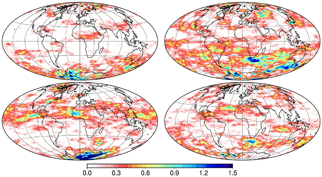
Figure 1. Sample of 4 vectors x from the prior probability distribution.

In our example, the prior probability distribution for x is only known through a sample of limited size m. In the reference example, the sample size is set to m = 100, but sensitivity experiments are performed with smaller m. In practical applications, it can indeed be very difficult to produce a large sample, especially if it is obtained from an expensive ensemble model simulation.

2.2. Observation System

Three types of observations of x(θ, ϕ) are assumed available:

(a) the value of x(θ, ϕ) at several locations (θ_j, ϕ_j), j = 1, …, p;

(b) the location of the maximum of x(θ, ϕ);

(c) the fraction of the surface of the sphere where x(θ, ϕ) is equal to zero.

Observations (a) are local, with a linear observation operator, while observations in (b) and (c) are non-local, with a non-linear (even non-differentiable) observation operator. In the example, they will be used jointly or separately to illustrate the ability of the method to deal with various types of observations.

Observations (a) are assumed unbiased, with observation errors following a gamma distribution (to keep observations positive). The observation error standard deviation is specified as a constant fraction of the expected value. In the example, this constant is set to ${\tilde{\sigma }}_a=20\%$.

Observation (b) is assumed unbiased, with observation errors following a Gaussian-like distribution on the sphere. In practice, it is generated by sampling a random azimuth for the perturbation with uniform distribution between 0 and 2π, and a random distance from the reference point, using a χ² distribution with 2 degrees of freedom for the square of the distance. The observation error standard deviation is specified as a fraction of the circumference of the sphere. In the example, it is set to ${\tilde{\sigma }}_b=5\%$ (which corresponds to an angle of 18°).

Observation (c) is assumed unbiased, with observation errors following a beta distribution (to keep observations between 0 and 1). The classic parameters α and β of the beta distribution are specified in terms of the mean $\mu =\frac{\alpha }{\alpha +\beta }$ and sample size ν = α + β, so that the observation error variance is equal to ${\sigma }^2=\frac{\mu (1-\mu )}{\nu +1}$, which can be specified by the maximum standard deviation ${\tilde{\sigma }}_c=\frac{1}{2\sqrt{\nu +1}}$ (occurring if μ = 0.5). In the example, it is set to ${\tilde{\sigma }}_c=0.1\%$.

In the application, the observations are simulated from a reference field x^t, hereafter called the true field. This true field is drawn from the probability distribution defined in section 2.1 (as the prior ensemble), but this is an independent additional draw, which is only used to simulate the observations and to evaluate the final results.

Figure 2 shows the true field x^t that is used throughout this paper, together with the spatial locations of observations (a), which have been sampled from a uniform density on the sphere. In the reference example used in the paper, the coverage ratio is set to ρ_a = 1/100 (one observation in every 10° × 10° box at the equator), which corresponds to a total of 420 observations on the sphere. The coverage of the local observations is here kept very sparse to better see the sensitivity of the results to localization and to the global observations, but experiments will be performed using denser observation networks (up to 659,839 local observations in the 1/4° grid).

FIGURE 2

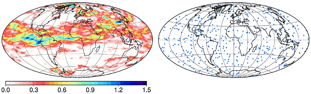
Figure 2. True field x^t (Left) and observation coverage (Right).

3. Ensemble Anamorphosis

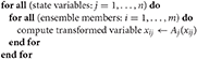
In this paper, a non-linear transformation is applied to all components of the vector x, so that their marginal distribution becomes a normalized Gaussian distribution ${N}(0,1)$. This condition on the marginal distribution is indeed a prerequisite to the application of the ensemble augmentation method and to the ensemble observational update presented in sections 4 and 5. The anamorphosis transformation A_i, associated to each variable x_i of the vector x, produces the transformed variable z_i = A_i(x_i). By combining these univariate transformations, we can write the transformed vector: z = A(x).

This section is organized as follows. In subsections 3.1 and 3.2, the algorithm to estimate the transformation A from the available ensemble and to apply the transformation is briefly summarized (see [24] for more details). In subsection 3.3, an extension of the algorithm is proposed to deal with the problem of discrete events.

3.1. Computation of the Transformation

Our basic assumptions to compute the transformation A are that: (i) the probability distribution of x is described by an ensemble of moderate size, so that the transformation A can only be approximately identified, and (ii) the size of the vector x can be very large so that the practical algorithm (to compute and apply A and A⁻¹) must contain as few operations as possible.

Let F(x) be the cumulative distribution function (cdf) corresponding to the marginal probability distribution of a variable x of the state vector, and G(z) be the cdf of the target distribution (the normalized Gaussian distribution in our case). Then, the forward and backward anamorphosis transformation, transforming x to z and z to x are given by:

$\begin{array}{ll}z=G^{-1}\left[F(x)\right]\text{and\hspace{1em}}x=F^{-1}\left[G(z)\right].& (4)\end{array}$

The whole problem thus reduces to estimating F(x) from the available ensemble.

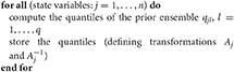
A simple and numerically efficient solution to this problem is to describe F(x) by a set of quantiles ${\tilde{x}}_k$ of the ensemble, corresponding to the ranks r_k, k = 1, …, q [i.e., such that $F({\tilde{x}}_k)=r_k$], and by linear interpolation between the quantiles. The transformation functions (corresponding to every variable x of the state vector) are thus completely described by the quantiles of the ensemble.

3.2. Application of the Transformation

The transformation is then piecewise linear and works by remapping the quantiles ${\tilde{x}}_k$ of the ensemble on the corresponding quantiles ${\tilde{z}}_k$ of the target distribution:

$\begin{array}{ll}A(x)={\tilde{z}}_k+\frac{{\tilde{z}}_{k+1}-{\tilde{z}}_k}{{\tilde{x}}_{k+1}-{\tilde{x}}_k}(x-{\tilde{x}}_k)\text{for\hspace{1em}}x\in \left[{\tilde{x}}_k,{\tilde{x}}_{k+1}\right],& (5)\end{array}$

$\begin{array}{ll}{A}^{-1}(z)={\tilde{x}}_k+\frac{{\tilde{x}}_{k+1}-{\tilde{x}}_k}{{\tilde{z}}_{k+1}-{\tilde{z}}_k}(z-{\tilde{z}}_k)\text{for\hspace{1em}}z\in \left[{\tilde{z}}_k,{\tilde{z}}_{k+1}\right].& (6)\end{array}$

This transformation is monotonous and bijective between the intervals $\left[{\tilde{x}}_1,{\tilde{x}}_q\right]$ and $\left[{\tilde{z}}_1,{\tilde{z}}_q\right]$, providing that the quantiles are all distinct (see section 3.3 for a generalization to non-distinct quantiles). The direct consequence of these properties is that anamorphosis transformation preserves the rank of the ensemble members and thus the rank correlation between variables (see [24] for more details about the effect of the transformation on correlations).

In principle, the transformation of x to z also requires including the backward transformation A⁻¹ in the observation operator to compute the observation equivalent: $\text{y}={H}\left[{\text{A}}^{-1}(\text{z})\right]$, where ${H}$ is the observation operator. Since A⁻¹ is non-linear by construction, this can be a problem if the observational update is unable to cope with a non-linear observation operator. In this case, a transformation must also be applied to observations y to keep a linear relationship between the transformed x and y. In this paper however, since the method described in section 5 can cope with a non-linear observation operator, no transformation of the observations is necessary. This greatly facilitates the application of anamorphosis transformation, since we will be able to use untouched observations, with their native non-Gaussian observation error probability distribution. Anamorphosis is only applied to the prior ensemble, not to the observations.

3.3. Discrete Events

In many practical applications, there can be problems in which a finite probability concentrates on some critical value x_c of the state variable. In this case the cdf F(x) is discontinuous and the standard anamorphosis transformation described by Equation (5) does not apply.

To generalize the algorithm, we can imagine the discontinuity in F(x) as the limit of a very steep slope (as illustrated in Figure 3). As long as there is a slope (left panel), we know which value of the rank r = F(x) corresponds to every value of x: a small uncertainty in x just produces a larger uncertainty in r when the slope is steeper. As soon as the slope becomes a step (right panel), we do not know anymore which rank r, between r_min and r_max, should correspond to x_c.

FIGURE 3

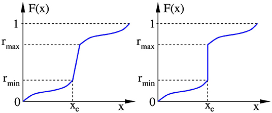
Figure 3. As long as there is a slope in the cdf (Left), we know which value of the rank r = F(x) corresponds to every value of x. As soon as the slope becomes a step at x_c (Right), we do not know anymore which rank r, between r_min and r_max, should correspond to x_c.

The solution is then to make the transformation stochastic and transform x to a random rank (with uniform distribution) between r_min and r_max: $z~{U}(r_{min},r_{max})$ for x = x_c. In this way, the forward transformation will transform the marginal distribution of all variables to the target distribution as required, the discrete events being transformed into a continuous variable by the stochastic transformation; and the backward transformation will transform it back to a discrete event, by transforming all ranks between r_min and r_max to x_c.

In the above scheme, it is important that the ranks r are sampled independently for different members, but not necessarily for different components x_i of x. We have thus the freedom to introduce spatial correlation in the sampling of the ranks r. If the transformed ensemble is meant to be updated with the assumption of joint Gaussianity (as will be done in section 5), a reasonable option is to avoid destroying the ensemble correlation structure where part of the members display the discrete event x = x_c. This can be done by using the same random rank for all variables from the same member. In this way, decorrelation can only be amplified where members move from a critical value (x = x_c) to a non-critical value (x ≠ x_c).

This is illustrated in Figure 4, showing the same 4 members as in Figure 1 after anamorphosis transformation. The marginal distributions are approximately Gaussian everywhere; the zero area is transformed to different values for different members (the rank is constant for a given member, but not the transformed value); discontinuities can occur along the border of the zero areas. The effect of the transformation on the correlation structure will be discussed later in section 4.1.

FIGURE 4

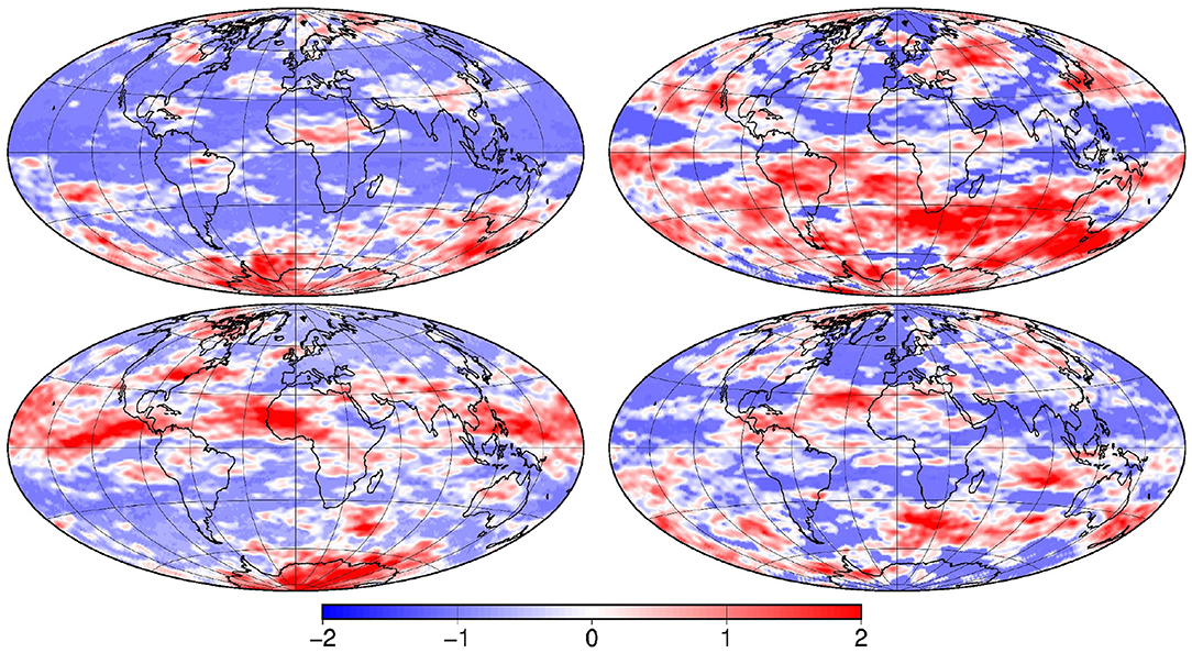
Figure 4. Anamorphosis transformation of the 4 vectors x displayed in Figure 1.

4. Ensemble Augmentation

A major difficulty with ensemble methods is that large ensembles are expensive to produce, while the accuracy of the statistics improves quite slowly with the ensemble size. Methods to artificially increase the ensemble size at low numerical cost can thus be very helpful. The approach that is used here to generate an augmented ensemble is to localize the correlation structure of the original ensemble using the modulation method described in Bishop et al. [13]. In this method, ensemble augmentation and localization are obtained together by computing each member of the augmented ensemble as the Schur product of one member of the prior ensemble with one column of the square root (or modal decomposition) of the localizing correlation matrix.

In the developments below, we will make use of the following property associated to this method: if x₁ and x₂ are two independent zero-mean random vectors with covariance C₁ and C₂, then the covariance of their Schur product x₁ ° x₂ is the Schur product of their covariance (C₁ ° C₂). Our plan is to apply this operation repetitively by computing the Schur product of one ensemble member with the large-scale patterns of several other members. In this way, localization will be obtained implicitly, in the sense that the characteristics of the localizing correlation matrix will depend on the statistical structure of the prior ensemble.

In this section and in the rest of the paper, it is assumed that the prior distribution is Gaussian, with zero mean and unit variance. This can be obtained by anamorphosis transformation as explained in the previous section. However, if the prior distribution is already close enough to being Gaussian, it can be better not to apply anamorphosis, but a linear transformation to center and reduce all variables. For this reason and to be compliant with the standard notation, we will keep using x as the name of the state vector, even if it corresponds to the transformed vector z from the previous section.

4.1. Localizing Correlations by Schur Products With Large-Scale Patterns

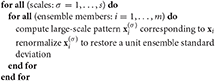
Let us suppose that every ensemble member x_i, i = 1, …, m is associated to its corresponding large-scale component ${\text{x}}_i^{(j)}$, for several truncation wave numbers j = 1, …, s, where s is the number of available large-scale patterns for each ensemble member. Then, we can construct multiple Schur products like:

$\begin{array}{ll}{\tilde{x}}_{\pi }=x_{\alpha }°\left(x_{\beta }^{(1)}°\dots °x_{\gamma }^{(1)}\right)°\dots °\left(x_{\psi }^{(s)}°\dots °x_{\omega }^{(s)}\right)& (7)\end{array}$

modulating one member of the original ensemble by the large-scale pattern of several other members. In computing this product, it is assumed that the member indices π = (α, β, …γ…ψ…ω) are all different so that the same member is never used twice in the same product.

Figure 5 illustrates large-scale patterns corresponding to the 4 transformed members displayed in Figure 4. They have been obtained by projecting the full-scale fields on the spherical harmonics, and by keeping only the large-scale components of the series, up to degree l₁ = 6. They are also renormalized to restore a unit ensemble standard deviation. In our reference example, only one truncation wave number (corresponding to degree l₁, illustrated in Figure 5) is used (s = 1), and the associated multiplicity is set to P₁ = 4. This means that the product is obtained by multiplying the original member with 4 large-scale patterns. In our experiments, l₁ is thus the only remaining parameter controlling localization, since s and P_j, j = 1, …, s are kept unchanged.

FIGURE 5

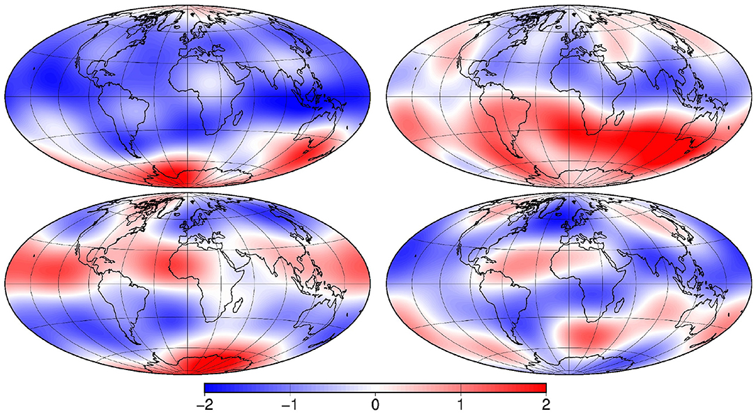
Figure 5. Large-scale pattern of the 4 transformed vectors displayed in Figure 4.

The covariance of ${\tilde{\text{x}}}_{\pi }$ is then:

$\begin{array}{ll}{\text{C}}_{\pi }=<{\tilde{\text{x}}}_{\pi }{\tilde{\text{x}}}_{\pi }^T>=\text{C}°\left({\text{C}}^{(1)}°\dots °{\text{C}}^{(1)}\right)°\dots °\left({\text{C}}^{(s)}°\dots °{\text{C}}^{(s)}\right)& (8)\end{array}$

where C is the correlation matrix of the original ensemble, and the rest of the product is the localizing correlation. One important condition on the localizing correlation matrix is that all elements must be non-negative, to avoid changing the sign of correlation coefficients in C. In Equation (8), this condition is easily verified by using an even Schur-power for each of the C^(j), j = 1, …, s. In this way, by using an even number of vector in each parenthesis of the product in Equation (7), we can be sure that we (implicitly) localize the ensemble covariance with a positive-element correlation matrix.

In Figure 6, this effect is illustrated by explicitly computing the correlation structure with respect to a reference location close to the equator in the Eastern Pacific. The first line displays the correlation C of the original ensemble (after anamorphosis transformation as displayed in Figure 4), computed with 100 members (left panel) and 500 members (right panel). We see that the long-range correlation structure is degraded if the ensemble size is reduced, so that localization is needed; and we note that the correlation structure remains smooth and regular despite the stochastic anamorphosis transformation (resulting from the probability peak at x = 0). The second line (left panel) displays the correlation C⁽¹⁾ of the corresponding large-scale patterns (displayed in Figure 5) and (right panel) the fourth Schur power of C⁽¹⁾, which is used as localizing correlation matrix. We see that it is everywhere positive (because of the even power), that the long-range correlations are reduced close to zero (because of the multiple product of small numbers), and that anisotropy is automatically taken into account (following the shape of the large-scale correlation structure). The third line (left panel) shows the localized correlation, again explicitly computed with Equation (8), i.e., as the Schur product of the top left and middle right panels of the figure. We see that localization is effective: the significant correlations are preserved and the long-range correlations are reduced close to zero. That the same effect can be obtained implicitly by ensemble augmentation remains to be checked (see section 4.2).

FIGURE 6

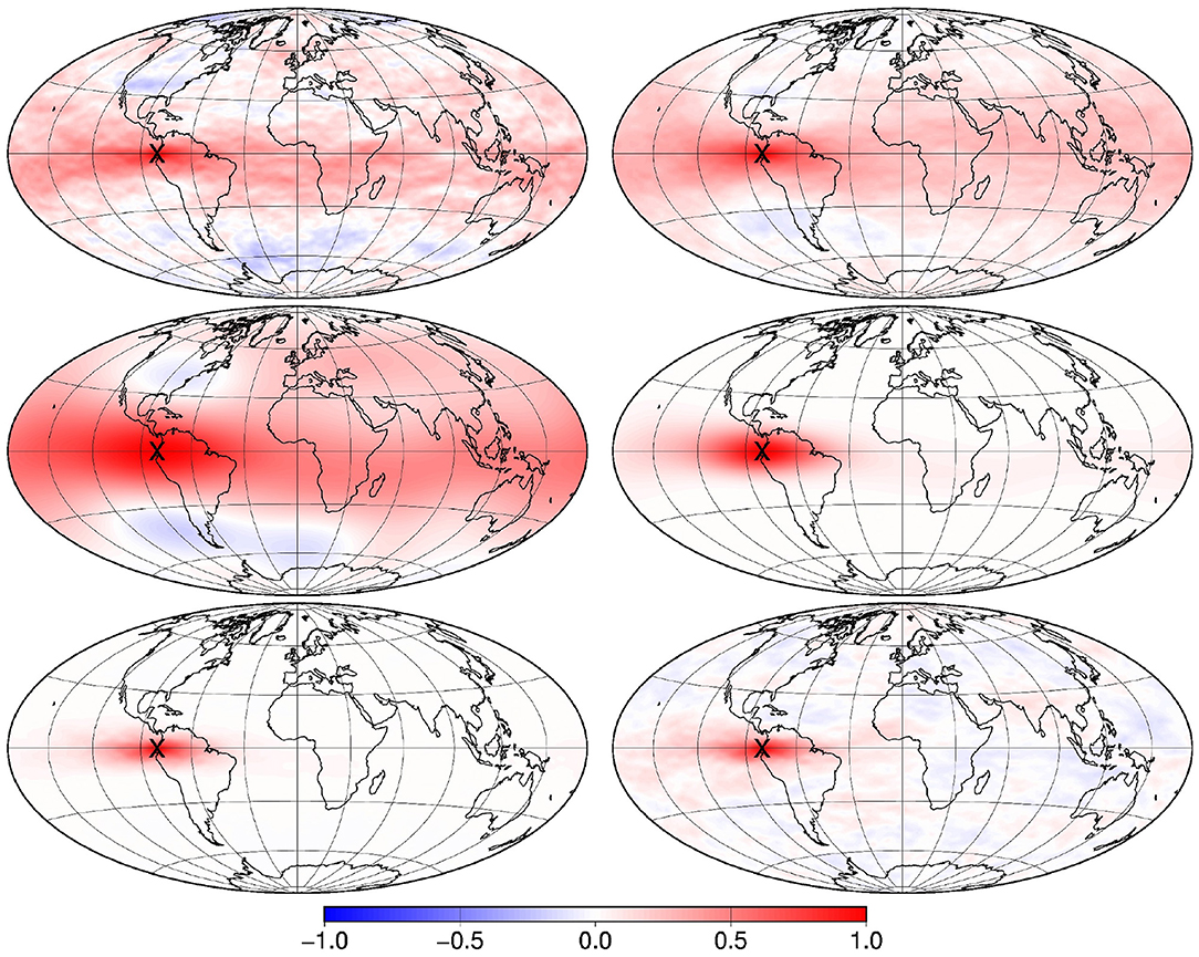
Figure 6. Correlation maps with respect to a reference location on the equator in the Eastern Pacific: 100-member prior correlation (top left), 500-member prior correlation (top right), 100-member correlation for the large-scale patterns (middle left), localizing correlation (middle right), localized correlation (bottom left) and correlation associated to a 500-member augmented ensemble (bottom right).

From the above discussion, it must be emphasized that the characteristics of the localizing correlation matrix intimately depend on the correlation structure of the multiscale prior ensemble. In this example, localization can be obtained because the prior ensemble correlations are decreasing with the distance to non-significant remote correlations, so that they can be reduced close to zero by P products (providing that P is large enough), while the local correlations can be preserved by using large-scale patterns. Such a decrease of the ensemble correlations with the distance is the very assumption supporting the use of localization itself, with the justification that it is quite a common behavior in many applications, but if very substantial remote correlations exist in the prior ensemble, they can be preserved by the implicit method that is proposed here, and something different from localization will be produced.

The key property of Equation (7) for augmenting the original ensemble is the very large number of vectors ${\tilde{\text{x}}}_{\pi }$ that can be generated by different combinations of the original members. With P Schur products (i.e., by combining P large-scale patterns to one original member), the number of possible combinations is:

$\begin{array}{ll}Ñ=\frac{m!}{(m-P-1)!{\displaystyle \prod _j}{P}_j!}\text{with }P\le m-1\text{and }{\displaystyle \sum _j}{P}_j=P& (9)\end{array}$

where m is the size of the original ensemble, P_j is the multiplicity of every scale j = 1, …, s in the product, and Ñ is the number of products that can be generated. For instance, for m = 100, P = 10 and all P_j (j = 1, …, 5) equal to 2, the maximum number of products that can be generated is as large as 100!/(89!2⁵) ≃ 1.767 × 10²⁰. The importance of the possibility to generate so many different products will be discussed later in section 5.1. For now, it is sufficient to see that, in our simple example, a full rank augmented ensemble can already be obtained with m = 20, s = 1 and P₁ = 4, since, in this case, Ñ = 77520, which is larger than the size of the state vector: n = 65160. By exploring the state space by linear combination of these products, we could solve the inverse problem globally without rank approximation.

4.2. Sampling of the Augmented Ensemble

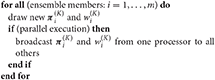
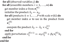
From the Schur products in Equation (7), members of the augmented ensemble can then be obtained by random linear combinations:

$\begin{array}{ll}{\text{x}}_i=\frac{1}{\sqrt{Ñ}}{\displaystyle \sum _{K=1}^{Ñ}}{w}_i^{(K)}{\tilde{\text{x}}}_{\pi (K)}& (10)\end{array}$

where x_π(K) is the Schur product obtained with combination π(K) of one original member and several large-scale patterns, and $w_i^{(K)}$ are independent random coefficients with ${N}(0,1)$ distribution. The augmented correlation structure is approximately given by Equation (8), and the marginal probability distributions are still ${N}(0,1)$, at the only condition that the variance of the x_π(K) is everywhere equal to 1, which follows directly from Equation (7).

In practice, the sum in Equation (10) is computed iteratively, as the result of the sequence:

$\begin{array}{ll}{\text{x}}_i^{(0)}=0;{\text{x}}_i^{(K+1)}={\alpha }_K{\text{x}}_i^{(K)}+{\beta }_K{w}_i^{(K)}{\tilde{\text{x}}}_{{\pi }_i(K)}& (11)\end{array}$

with

$\begin{array}{ll}{\alpha }_K=\frac{\sqrt{K}}{\sqrt{K+1}}\text{and\hspace{1em}}{\beta }_K=\frac{1}{\sqrt{K+1}}.& (12)\end{array}$

Equation (11) is exactly equivalent to Equation (10) if Ñ iterations are performed, except that we introduce an important modification: instead of browsing successively all possible combinations π(K), K = 1, …, Ñ of the members used in the Schur product, we draw a random combination π_i(K) from all possibilities at iteration K, and this draw is performed independently for every member i of the augmented ensemble. In this way, the augmented members are constructed iteratively by involving progressively more and more Schur products. The drawing of independent π_i(K) for different members speeds up the diversity of the members x_i in the augmented ensemble, even after a moderate number of iterations.

Figure 7 illustrates 4 vectors x_i from the augmented ensemble, as obtained after only N = 1000 iterations of Equation (11). This means that not all possible Schur products are combined to build each member of the augmented ensemble (since N ≪ Ñ). The vectors are displayed after backward anamorphosis transformation, so that they can be directly compared to the members of the original ensemble displayed in Figure 1. The comparison shows that the shape of the local structures looks similar in the augmented and original ensemble, but the large-scale structures that existed in the original ensemble are no more present in the augmented ensemble, as a result of localization. The correlation structure of the augmented ensemble (computed from 500 members) is displayed in Figure 6 (bottom right panel). We see that localization is effective, and very similar to the expected localized correlation computed with Equation (8) and displayed in the bottom left panel of the figure. The small remaining difference only results from the limited size of the augmented ensemble that has been used.

FIGURE 7

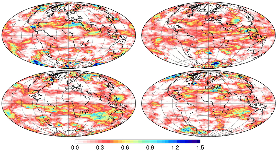
Figure 7. Sample of 4 vectors from the augmented ensemble.

5. Ensemble Observational Update

The observational update is based on the Bayes theorem:

$\begin{array}{ll}{p}^a(\text{x})=p(\text{x}|{\text{y}}^o)~p^b(\text{x})p({\text{y}}^o|\text{x})& (13)\end{array}$

where p^b(x) is the prior probability distribution for the state of the system, p(y^o|x) is the conditional probability distribution for the observations y^o given the state x of the system, and p^a(x) is the posterior probability distribution for the state of the system, conditioned to observations y^o.

In the following, it is assumed that p^b(x) is Gaussian, with ${N}(0,1)$ marginal distributions, and with a correlation structure described by the augmented ensemble (as described in the previous section); but no assumption is made on p(y^o|x), and thus on p^a(x). The objective of the observational update is to produce a sample of p^a(x).

5.1. Ensemble MCMC Algorithm

Equation (11) defines the transition probability distribution $q({\text{x}}_i^{(K+1)}|{\text{x}}_i^{(K)})$ of the MCMC chains, which rules the probability of transitioning from state ${\text{x}}_i^{(K)}$ to state ${\text{x}}_i^{(K+1)}$. From this definition, the expected value of ${\text{x}}_i^{(K+1)}$ is set to ${\alpha }_K{\text{x}}_i^{(K)}$, and the probability of the random perturbation is everywhere zero, except in the directions of the Ñ Schur products x_π. In these directions, the probability distribution is a univariate Gaussian, with standard deviation β_K (times the Euclidian norm of the Schur product). The transition probability distribution is thus not a regular n-dimensional probability distribution: it is made of a large number of one-dimensional distributions in many possible directions.

To modify the probability distribution sampled by a Markov chain, it is possible to transform the transition probability by introducing an acceptance probability $\theta ({\text{x}}_i^{(K+1)},{\text{x}}_i^{(K)})$:

$\begin{array}{ll}{q}^{\prime }({\text{x}}_i^{(K+1)}|{\text{x}}_i^{(K)})=q({\text{x}}_i^{(K+1)}|{\text{x}}_i^{(K)})\theta ({\text{x}}_i^{(K+1)},{\text{x}}_i^{(K)})& (14)\end{array}$

where q is now the proposal probability distribution, and q′, the transformed transition probability distribution. For instance, with any regular n-dimensional proposal probability distribution, we could obtain a Metropolis/Hastings algorithm to sample p^b(x), by using the acceptance probability:

$\begin{array}{ll}{\theta }^b({\text{x}}_i^{(K+1)},{\text{x}}_i^{(K)})=min\left\{\frac{p^b({\text{x}}_i^{(K+1)})q({\text{x}}_i^{(K)}|{\text{x}}_i^{(K+1)})}{p^b({\text{x}}_i^{(K)})q({\text{x}}_i^{(K+1)}|{\text{x}}_i^{(K)})},1\right\}.& (15)\end{array}$

This choice would verify the local balance condition q′(x′|x)p^b(x) = q′(x|x′)p^b(x′), which would ascertain the convergence of the chains toward a sample of p^b(x). On the contrary, with the singular transition probability in Equation (11), the local balance condition cannot be strictly verified, because there is no return path from ${\text{x}}_i^{(K+1)}$ to ${\text{x}}_i^{(K)}$. There is thus no guarantee that the Markov chains in Equation (11) rigorously converge toward a sample of the n-dimensional distribution p^b(x), or even that they converge toward a stationary distribution.

Despite of this, we here make the approximation that the local balance condition is verified in Equation (11). This means assuming that the contraction by the factor α_K together with the perturbation ${\beta }_K{w}^{(K)}$ along a random Schur product x_π is in approximate equilibrium with p^b(x) (locally in K). Thus, even if the asymptotic probability distribution sampled by the ensemble of Markov chains is not perfectly stationary, the fluctuations around p^b(x) are assumed negligible. In other words, what we do is to replace the classic multivariate n-dimensional proposal distribution (which would ensure local balance) by a large number of one-dimensional distributions (in many possible directions) and assume that this is not affecting too much the local balance condition. The accuracy of this approximation is likely to depend on the ability of the Ñ directions of perturbations to provide an appropriate pseudo-random sampling of the n-dimensional state space. For example, in our application, with m = 100 and P = 4, the number of sampling directions is Ñ ≃ 3.76 × 10⁸, which means that there are about 5,800 times more sampling directions than dimensions. This gives confidence that the approximation should be acceptable, even if further work is certainly needed to evaluate the quality of this approximation as a function of Ñ, and thus as a function of P.

With this assumption, it is then very easy to modify the Markov chains in Equation (11) to sample p^a(x) rather than p^b(x) using the same argument as in the Metropolis/Hastings algorithm. To satisfy the modified local balance condition q′(x′|x)p^a(x) = q′(x|x′)p^a(x′), we just need to introduce the acceptance probability:

$\begin{array}{ll}{\theta }^a({\text{x}}_i^{(K+1)},{\text{x}}_i^{(K)})=min\left\{\frac{p({\text{y}}^o|{\text{x}}_i^{(K+1)})}{p({\text{y}}^o|{\text{x}}_i^{(K)})},1\right\}& (16)\end{array}$

accounting for the modification of the observation likelihood, according to Equation (13). Draws increasing the observation likelihood (θ^a = 1) are always accepted, while draws decreasing the observation likelihood are only accepted with probability θ^a < 1. With this acceptance probability, we expect that the modified transition probability is in local balance with p^a(x), at the same level of approximation as the original transition probability with p^b(x).

In practice, to compute the acceptance probability θ^a, we introduce the observation cost function:

$\begin{array}{ll}{J}^o(\text{x})=-logp({\text{y}}^o|\text{x})& (17)\end{array}$

so that,

$\begin{array}{ll}{\theta }^a=min\left[exp(\delta J^o),1\right]\text{with\hspace{1em} }\delta J^o=J^o({\text{x}}^{(K+1)})-J^o({\text{x}}^{(K)})& (18)\end{array}$

where δJ^o is the variation of the cost function resulting from the perturbation of x^(K). In our example, the cost function is the sum of the contributions from the 3 types of observations (defined in section 2.2):

$\begin{array}{ll}{J}^o=J_a^o+J_b^o+J_c^o& (19)\end{array}$

where,

$\begin{array}{llll}{J}_a^o& =& -{\displaystyle \sum _{j=1}^p}logp\left\{y_{a,j}^o|{{H}}_{a,j}\left[{\text{A}}^{-1}(\text{x})\right]\right\}& (20)\end{array}$

$\begin{array}{llll}{J}_b^o& =& -logp\left\{y_b^o|{{H}}_b\left[{\text{A}}^{-1}(\text{x})\right]\right\}& (21)\end{array}$

$\begin{array}{llll}{J}_c^o& =& -logp\left\{y_c^o|{{H}}_c\left[{\text{A}}^{-1}(\text{x})\right]\right\}& (22)\end{array}$

correspond, respectively, to the gamma, normal and beta distributions associated to observations (a), (b) and (c). In the computation of J^o, inverse anamorphosis must be applied to x to go back to the original variables before applying the observation operators ${{H}}_{a,j}$, ${{H}}_b$, ${{H}}_c$ corresponding to the 3 types of observation.

Figure 8 illustrates 4 members from the updated ensemble, as obtained (after N = 10⁶ accepted draws) by introducing the acceptance probability (18) in the iteration of Equation (11). The vectors are displayed after backward anamorphosis transformation, so that they can be directly compared to the members of the prior ensemble (in Figure 1), to the members of the augmented ensemble (in Figure 7), and to the true state (in Figure 2). The comparison suggests that (i) the local correlation structure is similar in the prior and posterior ensemble (which indicates that it has been correctly used to fill the gap between observations), (ii) all members of the posterior ensemble have gained close similarity to the true state, (iii) the large-scale patterns of the true state are even quite adequately retrieved from the observation network (despite localization), (iv) the information brought by the observations has been sufficient to strongly reduce the spread of the posterior ensemble (as compared to the prior ensemble), (v) a significant posterior uncertainty remains, which needs to be quantitatively evaluated (see next subsection).

FIGURE 8

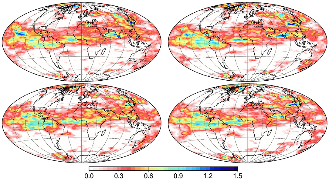
Figure 8. Sample of 4 vectors x from the updated ensemble.

Anticipating the final summary of the algorithm given in section 6.1, it must already be emphasized that the only inputs of the algorithm are: (i) the multiscale transformed prior ensemble (illustrated in Figures 4, 5), and (ii) the observations (with their associated error distributions). No other intermediate results, like the Schur products or the augmented ensemble members, need to be precomputed and stored. The posterior ensemble illustrated in Figure 8 is the direct result of the application of iteration (11), using Equation (7) to sample and compute a Schur product (from the multiscale prior ensemble) and Equations (17–20) to compute the acceptance probability (from the observations and their associated error distributions).

5.2. Evaluation of the Results

The standard protocol to evaluate the performance of ensemble simulations is to measure the reliability and the resolution of the ensemble using verification data [25, 26]. In our example, the true field x^t (displayed in Figure 2) will be used as verification data. Reliability is then a measure of the consistency of the ensemble with the true field x^t. By construction, the prior ensemble is perfectly reliable, since x^t is drawn from the same probability distribution. Resolution is a measure of the accuracy of the ensemble, or the amount of information that it provides about the true field. In our example, the prior ensemble does not provide much useful information about the true state; the resolution is thus poor. What is expected from the observational update is thus that the resolution can be improved (by the information brought by the observations), without degrading reliability.

In this paper, reliability and resolution will be measured using the continuous rank probability score (CRPS), following the decomposition of Hersbach [27]. Figure 9 (left and middle panels, red curve) shows for instance the evolution of the reliability and resolution of the updated ensemble as a function of the iteration index K in the Markov chains. From this figure, we see that (i) reliability is quickly obtained (after <100 iterations) and then deteriorates to a maximum (at about the same level of reliability as the prior ensemble) before improving slowly, and (ii) resolution steadily improves from the beginning to the end. This means that the ensemble spread is steadily reduced, but remains always sufficient to maintain consistency with the true state. The steady improvement of the solution (after reliability has reached its maximum) means that the intermediate ensembles (obtained before convergence, maybe after a few thousand iterations in this example), can be viewed as valuable approximations which can be produced and delivered more quickly than the optimal solution.

FIGURE 9

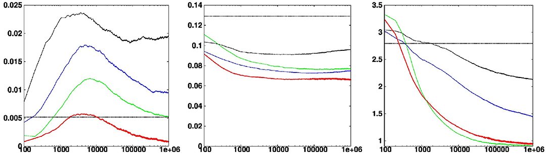
Figure 9. Reliability (Left), resolution (Middle) and optimality (Right) scores as a function of the number of accepted iterations. The scores are shown for the solutions obtained without localization (black curve), with optimal localization (l₁ = 6, red curve), with not enough localization (l₁ = 1, blue curve), and with too much localization (l₁ = 64, green curve). They can be compared to the score of the prior ensemble (thick dashed horizontal line).

The above scores tell us how much the updated ensemble has improved as compared to the prior ensemble, but they do not tell us if we made the best possible use of the available observations. Is the updated ensemble close enough to observations to be consistent with the probability distribution of observation errors? To evaluate this, we use the optimality score proposed in the Appendix. In short, this score is obtained by computing the rank $r_{ij}^o$ of every observation $y_j^o,j=1,\dots ,p$ in the probability distribution for observation errors $p(y_j^o|{\text{x}}_i)$, conditioned on every member x_i, i = 1, …, m of the ensemble. If optimality is achieved, this rank is uniformly distributed between 0 and 1. To obtain a single score, we transform this uniform number into a ${N}(0,1)$ number, and take the mean square, according to Equation (36). This defines the optimality score, which is expected to be equal to 1 (for p → ∞ and m → ∞).

Figure 9 (right panel) shows the evolution of this optimality score as a function of the iteration index K in the Markov chains. From this figure, we see that the score steadily improves from the beginning to the end, to reach a value that is close to 1 at convergence. This means that the updated ensemble is progressively moving close to the observations, but remains far enough at the end to be consistent with the probability distribution of observation errors.

The ensemble scores described above illustrate the steady improvement of the solution with the number of iterations. A key element of the algorithm is then to decide how many iterations to perform before stopping. This convergence criterion is application dependent and must be considered as an additional input of the algorithm (supplied by the user). In our example, the optimality score could be used to check convergence, because it is the main property of the method that we want to ascertain (and because the other scores defined above could not be used since they are based on the true field). In practice, the Markov chains could be stopped when the optimality score is below a given level or when its variation with K is below a prescribed tolerance.

5.3. Sensitivity to Localization and Ensemble Size

The only free parameters of the algorithm are the parameters controlling localization (through ensemble augmentation with Schur products). These parameters are: (i) the operators that are applied to obtain each scale of the multiscale ensemble from the original ensemble, and (ii) the number of times that each scale of the multiscale ensemble is used in the computation of the Schur product. In our example, only one additional scale is included in the multiscale ensemble, and it is used 4 times in the computation of the Schur products, so that there is only one remaining free parameter: the maximum degree l₁ that has been used to obtain the large-scale patterns (in Figure 5) from the original ensemble (in Figure 1). In the results discussed in sections 5.1 and 5.2, we used the value of l₁ for which the best scores have been obtained, but the quality of the results is very sensitive to l₁. The optimal tuning of the localization parameters is thus a very important problem.

First, we examine how the system behaves if the parameter l₁ is moved away from its optimal value. In Figure 9, the blue curve corresponds to less localization (larger l₁) and the green curve, to more localization (smaller l₁). In both cases, reliability is lost and resolution is worse. With not enough localization, the optimality score remains well above 1, which means that the updated members are unable to move close enough to the observations: the constraint imposed by the prior distribution is too strong, more localization is thus needed. With too much localization, the initial decrease of the optimality score is slower, because more degrees of freedom need to be adjusted to observations, but on the long run, the solution is moving closer to the observations. However, this is done at the price of reliability and resolution: less localization would improve the solution.

Second, we examine the variations of the scores at convergence, as a function of the localization parameter (l₁) and the ensemble size (m). In Figure 10, the variations of the final scores as a function of l₁ can be interpreted as explained above. In this figure, the red line corresponds to the nominal ensemble size (m = 100, used in all figures above), and the blue line corresponds to a smaller ensemble size (m = 50). With a smaller ensemble size, the optimal value of l₁ is slightly larger, since there are more non-significant correlations to eliminate by localization. The resolution and reliability are also worse, since there is less meaningful information coming from the augmented ensemble.

FIGURE 10

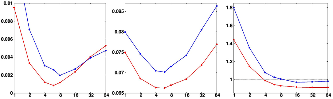
Figure 10. Final reliability (Left), resolution (Middle), and optimality (Right) scores as a function of localization degree l₁. The red line corresponds to the nominal ensemble size (m = 100, used in all figures above), and the blue line, to a smaller ensemble size (m = 50).

5.4. Impact of the Non-local/Non-linear Observations

To illustrate the impact of observing the location of the maximum of the field (observation $y_b^o$), Figure 11 shows the ensemble distribution for the location of the maximum, as obtained (a) from the prior ensemble (top left panel), (b) from the updated ensemble using the local observations only (top right panel), (c) from the updated ensemble using all observations (bottom left panel), and (d) from the updated ensemble using observation $y_b^o$ only (bottom right panel). In the prior ensemble, the probability to find the maximum is uniform in longitude, and increases with latitude (as a result of the increase of the standard deviation with latitude). With the local observations only, the uncertainty in the location of the maximum is already substantially reduced, but the posterior probability is still splitted into several distinct areas, which correspond to the areas where the true field is large, and between which the algorithm can hesitate in placing the maximum, if the local observation system is not dense enough. With all observations, most of the remaining uncertainty in the location of the maximum has been canceled (except in 3 or 4 members), which means that the constraint applied by the observation $y_b^o$ has been taken into account by the algorithm. With observation $y_b^o$ only, the posterior ensemble displays a wide variety of fields (very much like the prior ensemble, since $y_b^o$ is not very informative on the structure of the field), but all with their location of the maximum close to the observed location.

FIGURE 11

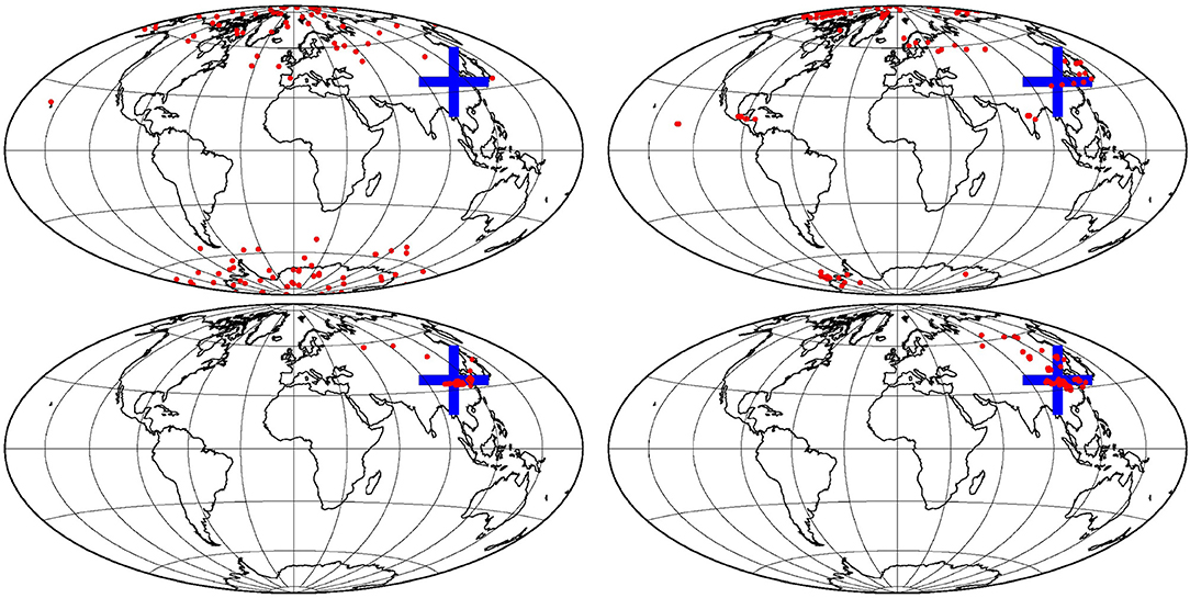
Figure 11. Distribution of the location of the maximum, as obtained: from the prior ensemble (top left), from the updated ensemble using the local observations only (top right), from the updated ensemble using all observations (bottom left), and from the updated ensemble using observation $y_b^o$ only (bottom right).

To illustrate the impact of observing the fraction of the sphere where the field is equal to zero (observation $y_c^o$), Figure 12 shows scatterplots of this fraction, as obtained (a) from the prior ensemble (top left panel), (b) from the updated ensemble using the local observations only (top right panel), (c) from the updated ensemble using all observations (bottom left panel), and (d) from the updated ensemble using observation $y_c^o$ only (bottom right panel). In this figure, we observe the same kind of behavior that was observed in Figure 11 for the location of the maximum: a large prior uncertainty, which is already substantially reduced by the local observations, and which is almost canceled out by the direct observation of $y_c^o$ (alone or together with all other observations). In this case, however, the verification of the global constraint on the zero surface (x-axis) does not mean that it is locally consistent with the true field (y-axis). This depends on the local observations; but we can see that the global constraint also helps improving the local consistency.

FIGURE 12

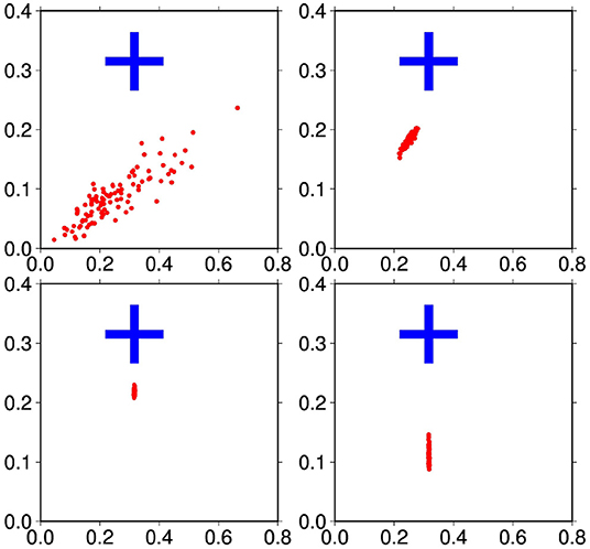
Figure 12. Distribution of the fraction of the sphere where the field is equal to zero (x-axis) and where both the field and the true field are equal to zero (y-axis), as obtained: from the prior ensemble (top left), from the updated ensemble using the local observations only (top right), from the updated ensemble using all observations (bottom left), and from the updated ensemble using observation $y_c^o$ only (bottom right).

These results suggest that the algorithm was able to deal adequately with the nonlocal/nonlinear/nondifferentiable observations $y_b^o$ and $y_c^o$. This was done by using statistics from a moderate size ensemble, complemented by a parameterized localization of the ensemble correlation structure. To cope with non-local observation operators, the problem is solved globally with implicit localization. To cope with non-linear/non-differentiable observation operators, the conditioning of the prior ensemble to the observations is performed using an ensemble of MCMC chains converging toward a sample of the posterior probability distribution.

6. Computational Complexity

This last section is dedicated to evaluating the numerical cost of the algorithm as a function of the dimension of the problem. This requires providing a final summary of the algorithm (in section 6.1), from which computational complexity formulas can be derived (in section 6.2). Lastly, scalability experiments are performed to evaluate the performance of the method as a function of the size of the problem (in section 6.3).

6.1. Summary of the Algorithm

The overall algorithm can be splitted into 3 phases: preprocessing, iteration of the Markov chains, postprocessing:

1. Preprocessing involves:

(a) Identification of the anamorphosis transformation functions:

(b) Anamorphosis of the prior ensemble:

(c) Scale separation in the prior ensemble:

2. For each iteration of the Markov chain (K = 1, …, N):

(a) Generate the random parameters required to compute perturbations:

(b) Compute and apply ensemble perturbations:

(c) Compute the observation cost function J^o:

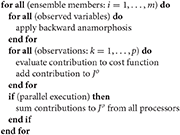
(d) Check if the perturbation is accepted:

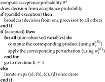
3. Postprocessing involves:

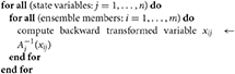
(a) Backward anamorphosis of the posterior ensemble:

One of the most salient feature of this algorithm is that most operations are performed independently for every state variable j = 1, …, n. The main exception is in step 1c (in the preprocessing): scale separation is the only step of the algorithm where the spatial location of the variables is taken into account and from which localization is subsequently obtained. Everywhere else, there is no direct coupling of the computations performed for two different state variables.

On the other hand, in step 2c, in the loop over observations (k = 1, …, p), the algorithm is computing J^o as the sum of contributions from every observations. This amounts to assuming that observation errors are independent. This is here needed to make the algorithm efficient enough, but solutions exist to relax this assumption (see conclusions).

With these two features (independence of the computations for every variable and every observation), the parallelization of the algorithm on a large number of processors is both very easy and very efficient. Each processor has only to deal with a small segment of the state vector and a small segment of the observation vector, and there need not be any special connections between the state variables and the observations that are treated by a given processor. Interactions between processors only involve:

• the broadcasting of the random parameters ${\pi }_i^{(K)}$ and $w_i^{(K)}$,

• the summing up of the contributions to the cost function J^o,

• the broadcasting of the acceptance decision,

and, in the presence of global observations:

• the exchange of the information required to apply the global observation operator.

6.2. Dependence Upon Problem Dimensions

If the number of iterations N is large, the overall cost of the algorithm is dominated by steps 2b, 2c and 2d. Their computational complexity (leading behavior for large size problems) can be estimated as follows:

$\begin{array}{ll}{C}_{2b}~\nu N{n}_{h}mP,C_{2c}~\nu Nm{C}_J,C_{2d}~N(n-n_h)mP& (23)\end{array}$

where N is the number of iterations (i.e., the number of accepted draws), νN is the total number of draws (i.e., including the rejected draws), n is the number of state variables, n_h is the number of state variables involved in the observation operator, m is the ensemble size, P is the number of Schur products, and C_J is the cost associated to the evaluation of the cost function J^o (including the backward anamorphosis transformation). In the case of local observations, C_J is proportional to the number p of local observations: C_J ~ pQ, where Q is the cost of the evaluation of J^o for one single observation.

To evaluate the complexity leading behavior C of the overall algorithm, three possibilities can be distinguished:

1. There are only local observations (n_h = p):

$\begin{array}{ll}C~\nu Nmp(P+Q).& (24)\end{array}$

If P and Q are of order 1, the cost C is then a moderate factor times νNmp. It is thus linear in m and p, but depends on the ability to keep νN inside reasonable bounds.

2. There are global observations, i.e., all state variables are necessary to compute the cost function (n_h = n):

$\begin{array}{ll}C~\nu NmnP+\nu Nm{C}_J.& (25)\end{array}$

If the second term ($C_J=pQ+C_J^{\mathrm{\text{glob}}}$) is negligible (as in our example), the cost is then proportional to m and n (rather than m and p).

3. There are no global observations, many non-observed variables and/or very few rejected draws (so that νn_h < n). In this case, the cost of step 2d can become dominant:

$\begin{array}{ll}C~NnmP.& (26)\end{array}$

In good approximation, the overall cost C of the algorithm thus depends on the size of the problem (proportional to mp in case 1 or to mn in cases 2 and 3) and the number of iterations or draws that are necessary to reach the solution (νN in cases 1 and 2 or N in case 3).

The linearity of the cost in m and p or in m and n is the key feature of this algorithm. This is not straightforward to obtain because the probability distribution to sample must be constrained by the covariance structure of the prior ensemble, with appropriate localization. In such a situation, the classic approach to generate perturbations with an adequate correlation structure is to compute linear combinations of ensemble members and to apply localization operators. In the context of an MCMC sampling algorithm, this would make the sampling of the proposal distribution of the algorithm much too expensive to be applicable to large-size problems. Conversely, the use of a non-regular proposal distribution that can be sampled by computing the Schur product of P vectors (P ≪ m) is the approximation that reduces the cost of the sampling to Pp or Pn (i.e., independent of m and of the localization scale). This simple scheme accounts for the structure of the prior probability distribution (i.e., the ensemble covariance, with localization), at a cost that is similar to the cost of the evaluation of the observation cost function for local observations (a factor P against a factor Q). The cost of each iteration is thus made about as small as it can be.

As a comparison, the computational complexity (leading behavior for large size problems) of the Local Ensemble Transform Kalman filter (LETKF, with domain localization, or LETKFm, with modulation to approximate covariance localization), and of the Local Ensemble Kalman filter (LEnKF, with covariance localization) can be written:

$\begin{array}{ll}{C}_{LETKF}~m^{2}pd,C_{LETKFm}~m^{2}pd{\rho }_a^2,C_{LEnKF}~m^{2}pd{\rho }_o^2& (27)\end{array}$

where m is the ensemble size, p is the total number of observations, d is the average number of local domains in which each observation is used, ρ_a is the ensemble augmentation ratio (resulting from modulation), and ρ_o is the root mean square ratio between the number of observations used in every local domain and the ensemble size. These complexity formulas stem from the assumptions that, in each local domain, the leading cost of the ETKF is proportional to the number of observations times the square of the ensemble size (to obtain the transformation matrix), and the leading cost of the EnKF is proportional to the cube of the number of observations (to perform the inversion in the observation space).

To compare with the MCMC sampler, in the case of local observations only, with complexity (24), we compute the number of iterations than could be performed to reach the same cost as each of these algorithm:

$\begin{array}{l}{N}_{LETKF}~\frac{md}{\nu (P+Q)},N_{LETKFm}~\frac{md{\rho }_a^2}{\nu (P+Q)},\\ N_{LEnKF}~\frac{md{\rho }_o^2}{\nu (P+Q)}.& (28)\end{array}$

For instance, with the following numbers: m ~ 100, d ~ 10000 (similar to the localization used in our example application), ν ~ 10 (about the ratio obtained in our application when there are many observations, see Table 1), P + Q ~ 10 (assuming Gaussian observation errors, as in the Kalman filters, so that Q is kept small), ρ_a ~ 10 (a modest augmentation ratio) and ρ_o ~ 10 (only 10 times more observations than in our reference example, which was poor in local observations), we obtain:

$\begin{array}{ll}{N}_{LETKF}~10^4,N_{LETKFm}~10^6,N_{LEnKF}~10^6.& (29)\end{array}$

The question of the cost then depends on the number of iterations that is necessary to reach a similar performance, in terms of reliability, resolution and optimality. This is likely to be very dependent on the specificities of every particular application. For instance, the number of iterations required is certainly much smaller if the prior ensemble is already quite consistent with the observations (as in a warmed up ensemble data assimilation system), as compared to our example application, in which the prior ensemble is very uninformative. From the above formulas, we can also see that the cost of traditional localization is proportional to the number of times (d) each observation is used, and thus to the square of the localization radius (in two dimensions), whereas in the MCMC sampler, the cost of localization is independent of the localization radius. The MCMC sampler is thus probably less efficient if the decorrelation length scales are small and if the observations can only produce a local effect, but it can also be viewed as a possible option to apply covariance localization at a lesser cost to problems that are more global and that require larger localization scales.

TABLE 1

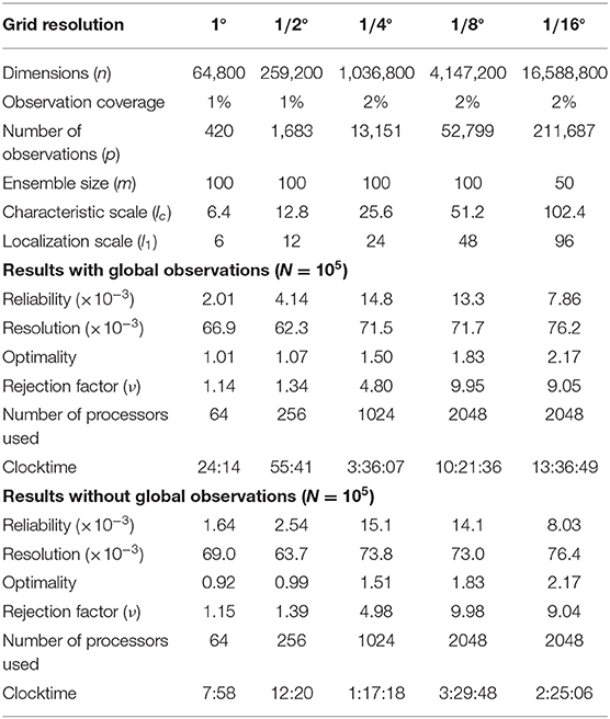
Table 1. Dependence of the solution on the size of the problem.

6.3. Scalability Experiments

Tables 1, 2 summarize the result of scalability experiments that have been performed by varying the number of dimensions (in Table 1) and the number of observations (in Table 2). The number of dimensions is increased by refining the resolution of the discretization grid (from 1° to 1/2°, 1/4°, 1/8°, and 1/16°), and by decreasing all length scales proportionally (i.e., the characteristic length scale of the random field 1/l_c and the localization length scale 1/l₁). The observation coverage is increased from 1 to 2% between the 1/2° and the 1/4° grids for technical reasons (to be sure to have at least one observation associated to the subdomain of each processor). The ensemble size is decreased from 100 to 50 members between the 1/8° and the 1/16° grids to reduce the memory requirement. The impact of the number of observations (in Table 2) is studied using the 1/4° grid, without global observations and with a reduced number of iterations (5 × 10⁴ instead of 10⁵).

TABLE 2

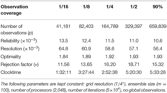
Table 2. Dependence of the solution on observation coverage.

Visually, the results of all these experiments look similar to what is shown in this paper for the 1° grid. Only the scale is different and there is thus a lot more structures on the whole sphere, but the spread and structure of the prior and updated ensembles as well as the closeness between the posterior members and the true field look similar. However, looking at the quantitative scores (reliability, resolution, optimality), we see that the solution is generally worsening as the size of the problem increases. The optimality score, in particular, indicates that the updated ensemble is further away from the observations (up to 2.17 times the observation error variance for the 1/16° experiment, which corresponds to an rms difference with observations about 50% too large). The reason for this is certainly that more iterations are needed to reach convergence in problems that have more degrees of freedom that can be controlled by the available observations. In this case, this has no obvious effect on the visual evaluation of the solution because the improvement of the resolution score remains quite good whatever the grid resolution, from about 0.13 for the prior ensemble (for all grids) to about 0.07 for the updated ensemble (from about 0.065 for the coarse grids to about 0.075 for the fine grids). This analysis of the scores is confirmed in Table 2, where the reliability and resolution scores are steadily improving using more and more observations (for a given number of iterations), while optimality is more and more difficult to achieve.

Similarity, for the global constraints, the results of the experiments show that the control of the position of the maximum is still effective at all grid resolution, even if, for the finest grids (1/4°, 1/8°, and 1/16°), the residual error becomes progressively too large as compared to observation error. On the contrary, the control of the surface where the field is equal to zero remains good for the coarse grids (1° and 1/2°), quite effective on the 1/4° grid, but is suddenly completely lost in the finest grids (1/8° and 1/16°), probably because the solution is still too far from convergence.

Clocktimes provided in the tables are only indicative of the numerical cost because they somehow depend on the changing behavior of the computer, and because these experiments are not intended to provide an accurate measure of the computational scalability of the algorithm. In principle, according to the complexity formulas, the cost should be proportional to the product of p, m and ν, divided by the number of processors (which are the only relevant parameters varying in these experiments). As a departure to this rule, we observe in the tables that the clocktime also decreases with the number of observations per processor, which suggests that the cost of communications (performed for each of the νNm evaluations of the cost function) is here non-negligible. It must also be noted that these experiments involved the non-Gaussian features of the algorithm (non-Gaussian observation error and backward anamorphosis transformation in the observation operator), which can lead to a cost one order of magnitude larger, as compared to Gaussian problems (because of the larger Q factor in the complexity formulas).

Overall, what we can conclude is that the number of iterations N required to reach convergence and the rejection factor ν are growing with the size of the problem, when a lot of information must be extracted from the observations. This can be traced back to the Markov chains in Equation (11), which are very well suited to sample the prior distribution (ν = 1, small N), but less and less efficient if the posterior distribution is more and more different from the prior distribution. One possible approach to reduce this difficulty could thus be to split the observation vector into pieces (assuming independent observation errors), and apply the whole algorithm (including preprocessing and postprocessing, as explained in section 6.1) serially to each piece of the observation vector. In this way, the information gain at each step would be smaller, and the efficiency of the overall algorithm could be improved.

7. Conclusions

In this paper, an approximate variant of the Metropolis/Hastings algorithm has been proposed to sample the posterior probability distribution of a Bayesian inverse problem. It was thought as a possible alternative to the ensemble observational update that is applied in local ensemble Kalman filters, but the range of possible applications may be wider. The main assumption of the algorithm is in the shape of the prior probability distribution, which is assumed jointly Gaussian (possibly after anamorphosis transformation accounting for non-Gaussian marginal distributions). As compared to more general methods (like particle filters), this is the price to pay to make the method more efficient and less demanding in terms of ensemble size. As compared to less general methods (like localized Kalman filters), the main benefit is that no assumption is made on the posterior distribution, so that non-linear data constraints are possible. The method also offers the following possibilities or perspectives, which could not be discussed in this paper.

7.1. Multivariate State Vector

In principle, the method is directly generalizable to problems involving several variables, spanning several dimensions, including time, even if this should be verified in practice (especially if anamorphosis is applied). Localization can indeed be applied (or not) along each dimension by using appropriate scale separation operators. Correlations between different variables (or along any dimension) can be kept untouched by localization (as in local ensemble Kalman filters) by using the same modulation patterns for all variables (or for all slices).

7.2. Scale Separation Operator

The modulation patterns used in the Schur products can be obtained in several other ways, for instance by sampling patterns with a specified global correlation matrix (explicit localization) or by using different sorts of scale separation operators. It might even be imagined to use a wider class of “simplification” operators, the main condition being probably that they have to remove structures from the original members, i.e., to decrease entropy of the prior Gaussian distribution.

7.3. Correlated Observation Errors

In the evaluation of the computational complexity in section 6, it was assumed that observation errors were independent. This limitation can possibly be relaxed by augmenting the observation vector with dependent observations (as proposed by [28] for Gaussian errors, using derivatives of the original observations). This can be an appropriate compromise as long as the numerical cost remains linear in the number of observations.

7.4. Size of the Updated Ensemble

To simplify the presentation, it has been assumed throughout the paper that the size of the updated ensemble is the same as the size of the prior ensemble, but this is not a limitation of the method. The size of the updated ensemble is freely adjustable; updated members can be computed altogether or separately; and more updated members can be added at will if needed. In this case, the cost of the algorithm depends on the size of the updated ensemble, not on the size of the prior ensemble.

7.5. Multiscale Applications

Multiscale structures can be incorporated in the algorithm in at least three ways: (i) by directly constraining the spectral amplitudes, considered as global observations (as in [22]), (ii) by including more than one large-scale in the Schur product in Equation (7), to obtain a multiscale localizing correlation, and (iii) by explicitly including large-scale products (for instance combining only s = 2 and s = 3) in the definition of the augmented ensemble in Equation (10). In the latter case, the proposal distribution would include a specified proportion of large-scale perturbations, which might speed up the convergence of the large scales.

7.6. Dynamical Constraints

Another important asset of the MCMC sampler is the possibility to cope with non-local/non-linear dynamical or structural constraints. They can be introduced as additional terms in the cost function to complement and distort the prior Gaussian distribution (using the same approach as [29]). The main limitation is that they must be cheap enough to be evaluated a large number of times. Low-complexity models can be explicitly included in the iterative inversion process, to cope with prominent dynamical features, while full-complexity models can only be used externally as a constraint to the moderate-size prior ensemble.

Data Availability Statement

The datasets generated for this study will not be made publicly available The datasets can be directly reproduced by the code, which is made publicly available.

Author Contributions

J-MB developed the method, performed the experiments, and wrote the paper.

Funding

This work benefited from support from the Copernicus Marine Environment Monitoring Service (CMEMS), in the context of the GLO-HR-ASSIM project. CMEMS is implemented by Mercator Ocean International in the framework of a delegation agreement with the European Union. The calculations were performed using HPC resources from GENCI-IDRIS (grant 2018-011279).

Conflict of Interest

The author declares that the research was conducted in the absence of any commercial or financial relationships that could be construed as a potential conflict of interest.

References

1. Evensen G. Sequential data assimilation with a non linear quasigeostrophic model using Monte Carlo methods to forecast error statistics. J Geophys Res. (1994) 99:10 143–10 162.

Google Scholar

2. Houtekamer PL, Mitchell HL. A sequential ensemble Kalman filter for atmospheric data assimilation. Mon Wea Rev. (2001) 129:123–37. doi: 10.1175/1520-0493(2001)129<0123:ASEKFF>2.0.CO;2

CrossRef Full Text | Google Scholar

3. Houtekamer PL, Zhang F. Review of the ensemble Kalman filter for atmospheric data assimilation. Mon Wea Rev. (2016) 144: 4489–532. doi: 10.1175/MWR-D-15-0440.1

CrossRef Full Text | Google Scholar

4. Sakov P, Counillon F, Bertino L, Lisæter KA, Oke PR, Korablev A. TOPAZ4: an ocean-sea ice data assimilation system for the North Atlantic and Arctic, Ocean Sci. (2012) 8:633–56. doi: 10.5194/os-8-633-2012

CrossRef Full Text | Google Scholar

5. Rasmussen J, Madsen H, Jensen KH, Refsgaard JC. Data assimilation in integrated hydrological modeling using ensemble Kalman filtering: evaluating the effect of ensemble size and localization on filter performance, Hydrol Earth Syst Sci. (2015) 19:2999–3013. doi: 10.5194/hess-19-2999-2015

CrossRef Full Text | Google Scholar

6. Bishop CH, Etherton BJ, Majumdar SJ. Adaptive sampling with the ensemble transform Kalman filter. Part i: theoretical aspects. Month Weather Rev. (2001) 129:420–36. doi: 10.1175/1520-0493(2001)129<0420:ASWTET>2.0.CO;2

CrossRef Full Text | Google Scholar

7. Pham DT, Verron J, Roubaud MC. Singular evolutive extended Kalman filter with EOF initialization for data assimilation in oceanography. J Mar Syst. (1998) 16:323–40.

Google Scholar

8. Ott E, Hunt B, Szunyogh I, Zimin A, Kostelich E, Corazza M, et al. A local ensemble Kalman filter for atmospheric data assimilation. Tellus. (2004) 56A:415–28. doi: 10.3402/tellusa.v56i5.14462

CrossRef Full Text | Google Scholar

9. Hunt B, Kostelich E, Szunyogh I. Efficient data assimilation for spatiotemporal chaos: a local ensemble transform Kalman filter. Phys D. (2007) 230:112–26. doi: 10.1016/j.physd.2006.11.008

CrossRef Full Text | Google Scholar

10. Bishop CH, Hodyss D. Ensemble covariances adaptively localized with ECO-RAP. Part 2: a strategy for the atmosphere. Tellus A. (2009) 61:97–111. doi: 10.1111/j.1600-0870.2008.00372.x

CrossRef Full Text | Google Scholar

11. Janjic Pfander T, Nerger L, Albertella A, Schröter J, Skachko S. On domain localization in ensemble-based Kalman filter algorithms. Mon Wea Rev. (2011) 139:2046–60. doi: 10.1175/2011MWR3552.1

CrossRef Full Text | Google Scholar

12. Bocquet M. Localization and the iterative ensemble Kalman smoother. Q J R Meteorol Soc. (2016) 142:1075–89. doi: 10.1002/qj.2711

CrossRef Full Text | Google Scholar

13. Bishop CH, Whitaker JS, Lei L. Gain form of the ensemble transform Kalman filter and its relevance to satellite data assimilation with model space ensemble covariance localization? Month Wheather Rev. (2017) 145:4575–92. doi: 10.1175/MWR-D-17-0102.1

CrossRef Full Text | Google Scholar

14. Farchi A, Bocquet M. On the efficiency of covariance localisation of the ensemble Kalman filter using augmented ensembles. Front Appl Math Stat. (2019) 5:3. doi: 10.3389/fams.2019.00003

CrossRef Full Text | Google Scholar

15. Zhu J, Zheng F, Li X. A new localization implementation scheme for ensemble data assimilation of non-local observations. Tellus. (2011) 63A:244–55. doi: 10.1111/j.1600-0870.2010.00486.x

CrossRef Full Text | Google Scholar

16. Barth A, Yan Y, Alvera-Azcárate A, Beckers JM. Local ensemble assimilation scheme with global constraints and conservation. Ocean Dynamics. (2016) 66:1651–64. doi: 10.1007/s10236-016-0999-y

CrossRef Full Text | Google Scholar

17. Zhou Y, McLaughlin D, Entekhabi D, Ng GHC. An ensemble multiscale filter for large nonlinear data assimilation problems. Mon Wea Rev. (2008) 136:678–98. doi: 10.1175/2007MWR2064.1

CrossRef Full Text | Google Scholar

18. Miyoshi T, Kondo K. A multi-scale localization approach to an ensemble Kalman filter. SOLA. (2013) 9:170–3. doi: 10.2151/sola.2013-038

CrossRef Full Text | Google Scholar

19. Li Z, McWilliams JC, Ide K, Farrara JD. A multiscale variational data assimilation scheme: formulation and illustration. Mon Wea Rev. (2015) 143:3804–22. doi: 10.1175/MWR-D-14-00384.1

CrossRef Full Text | Google Scholar

20. Caron JF, Buehner M. Scale-dependent background error covariance localization: evaluation in a global deterministic weather forecasting system. Mon Wea Rev. (2018) 146:1367–81. doi: 10.1175/MWR-D-17-0369.1

CrossRef Full Text | Google Scholar

21. Buehner M. Evaluation of a spatial/spectral covariance localization approach for atmospheric data assimilation. Mon Wea Rev. (2012) 140:617–36. doi: 10.1175/MWR-D-10-05052.1

CrossRef Full Text | Google Scholar

22. Tissier AS, Brankart JM, Testut CE, Ruggiero G, Cosme E, Brasseur P. A multiscale ocean data assimilation approach combining spatial and spectral localisation, Ocean Sci. (2019) 15:443–57. doi: 10.5194/os-15-443-2019

CrossRef Full Text | Google Scholar

23. Robert C, Casella P. Monte Carlo Statistical Methods. New York, NY: Springer (2004). 645 p.

Google Scholar

24. Brankart JM, Testut CE, Béal al D, Doron M, Fontana C, Meinvielle M, et al. Toward an improved description of ocean uncertainties: effect of local anamorphic transformations on spatial correlations. Ocean Sci. (2012) 8:121–42. doi: 10.5194/os-8-121-2012

CrossRef Full Text | Google Scholar

25. Candille G, Talagrand O. Evaluation of probabilistic prediction systems for a scalar variable. Quart J Roy Meteor Soc. (2005) 131:2131–50. doi: 10.1256/qj.04.71

CrossRef Full Text | Google Scholar

26. Candille G, Côté C, Houtekamer PL, Pellerin G. Verification of an ensemble prediction system against observations. Mon Wea Rev. (2007) 135:2688–99. doi: 10.1175/MWR3414.1

CrossRef Full Text | Google Scholar

27. Hersbach H. Decomposition of the continuous ranked probability score for ensemble prediction systems. Wea Forecast. (2000) 15 :559–70. doil doi: 10.1175/1520-0434(2000)015<0559:DOTCRP>2.0.CO;2

CrossRef Full Text | Google Scholar

28. Brankart JM, Ubelmann C, Testut CE, Cosme E, Brasseur P, Verron J. Efficient parameterization of the observation error covariance matrix for square root or ensemble Kalman filters: application to ocean altimetry. Mon Wea Rev. (2009) 137:1908–27. doi: 10.1175/2008MWR2693.1

CrossRef Full Text | Google Scholar

29. Brasseur P. A variational inverse method for the reconstruction of general circulation fields in the northern Bering Sea. J Geophys Res Oceans. (1991) 96:4891–907. doi: 10.1029/90JC02387

CrossRef Full Text | Google Scholar

30. Talagrand O. A posteriori verification of analysis and assimilation algorithms, in: Workshop on diagnosis of data assimilation systems. Reading: ECMWF (1999).

Google Scholar

Appendix

Optimality Score

Let x be the random vector describing the state of the system (in state space, of dimension n), and y be the random vector describing related observed quantities (in observation space, of dimension p). y is related to x by the stochastic observation operator ${H}$:

$\begin{array}{ll}\text{y}={H}(\text{x},ϵ)& (\mathrm{A1})\end{array}$

where ϵ is a random vector describing uncertainties in the observation system. This may include the classic additive observation error, but also more intricate sources of uncertainty in the modeling assumptions supporting the relation between x and y.

Let p(x) be the prior probability density function (pdf) for the state of the system, and p(y|x) be the conditional pdf for the observed quantities, given the state of the system. This conditional pdf describes the effect of uncertainties in the observation system in Equation (30). Then, the joint pdf for x and y can be written in two ways:

$\begin{array}{ll}p(\text{x},\text{y})=p(\text{x})p(\text{y}|\text{x})=p(\text{y})p(\text{x}|\text{y})& (\mathrm{A2})\end{array}$

where p(y) is the prior pdf for y, and p(x|y) is the conditional pdf for x, given y.

Given observations y^o, the posterior pdf for the state of the system is then given by:

$\begin{array}{ll}p(\text{x}|\text{y}={\text{y}}^o)=\frac{p(\text{x},{\text{y}}^o)}{p({\text{y}}^o)}=\frac{p(\text{x})p({\text{y}}^o|\text{x})}{p({\text{y}}^o)}.& (\mathrm{A3})\end{array}$

This corresponds to extracting a slice in p(x, y) at y = y^o, normalized by the constant p(y^o). For high-dimension problems (large n and p), this operation may become expensive and may thus require approximations in p(x), in p(y|x) and in the method used to extract the appropriate slice from p(x)p(y|x). Approximations in p(x) include for instance the use of a Gaussian model to describe the pdf, and the use of a moderate size ensemble (possibly augmented by a localization assumption) to estimate the Gaussian parameters. If these approximations are correct, then the posterior pdf p(x|y = y^o) must be consistent with the assumptions made about the dependence between x and y, i.e., with the assumptions made in Equation (30). This means that the density of the possible y resulting from p(x|y = y^o), through p(y|x), must be consistent with y^o.

However, as usual, checking this consistency would in principle require a large number of possible observation vectors y^o resulting from independent experiments applied to the system. The posterior pdfs p(x|y = y^o) resulting from each of these y^o would browse many possible slices p(x, y^o) in p(x, y), so that the consistency could be checked by computing statistics over many possible y^o. In practice, however, we assume here that we have only one observation vector y^o, so that we need to replace the statistics over many possible y^o by statistics over the components $y_j^o,j=1,\dots ,p$ of y^o. To do this, we need to assume that their observational uncertainties are independent:

$\begin{array}{ll}p(\text{y}|\text{x})={\displaystyle \prod _{j=1}^p}p(y_j|\text{x})& (\mathrm{A4})\end{array}$

and to define a statistics that is identically distributed for all j, so that the results obtained for different j can be mixed to compute an aggregate score.

One first statistics that would be appropriate to check that the posterior pdf is consistent with observational uncertainty is:

$\begin{array}{ll}{C}_{ij}^o=-log\left[p(y_j^o|{\text{x}}_i)\right]& (\mathrm{A5})\end{array}$

where x_i, i = 1, …, m is sampled from the posterior pdf (i.e., one member of the updated ensemble in our case). This statistics would be interesting because it is the contribution of $y_j^o$ to the cost function associated to member x_i, and because its expected value is the conditional entropy of y_j with respect to x. However, the probability distribution for C_ij is not identical for all i and j, and would need to be transformed before computing a global score.

To obtain a more practical score, another option is to compute:

$\begin{array}{ll}{r}_{ij}^o=P(y_j^o|{\text{x}}_i)& (\mathrm{A6})\end{array}$

where P(y_j|x) is the cumulative distribution function corresponding to p(y_j|x). r_ij is thus the rank of the observation $y_j^o$ in the conditional distribution for y_j, given the ensemble member x_i. For a pair (x, y) sampled from p(x, y) in Equation (31), this rank is uniformly distributed between 0 and 1 (by construction of y from x), so it must be for a random x_i sampled from a random slice at y = y^o. Here, the random y^o has been replaced by using independent components $y_j^o$ of y^o. It is thus important to note that $r_{ij}^o$ must not be uniformly distributed between 0 and 1 for every j, but only if enough independent $y_j^o$ have been used. Finally, to obtain one single score rather than a set of ranks, we transform the r_ij into Gaussian numbers, and compute the mean square according to:

$\begin{array}{ll}{z}_{ij}^o=G^{-1}(r_{ij}^o);\overline{z^2}=\frac{1}{mp}{\displaystyle \sum _{i=1}^m}{\displaystyle \sum _{j=1}^p}{z_{ij}^o}^2.& (\mathrm{A7})\end{array}$

The final score is then $\overline{z^2}$, which must be equal to 1, for m → ∞ and p → ∞. A score below one means that the updated ensemble is too close to the observations, and a score above one means that the updated ensemble is too far from the observations.

In the particular case of an additive Gaussian observational uncertainty:

$\begin{array}{ll}{y}_j={{H}}_j(\text{x})+{ϵ}_j\text{with\hspace{1em}}p({ϵ}_j)=\frac{1}{\sqrt{2\pi {\sigma }_j^2}}exp\left[-\frac{1}{2}\frac{{ϵ}_j^2}{{\sigma }_j^2}\right]& (\mathrm{A8})\end{array}$

where σ_j is the observation error standard deviation associated to y_j, the score $\overline{z^2}$ reduces to:

$\begin{array}{ll}\overline{z^2}=\frac{1}{mp}{\displaystyle \sum _{i=1}^m}{\displaystyle \sum _{j=1}^p}{\left(\frac{y_j^o-{{H}}_j({\text{x}}_i)}{{\sigma }_j}\right)}^2& (\mathrm{A9})\end{array}$

which exactly corresponds to checking the average value of the cost function:

$\begin{array}{ll}\overline{z^2}=\frac{2}{mp}{\displaystyle \sum _{i=1}^m}{\displaystyle \sum _{j=1}^p}\left[C_{ij}^o-log\sqrt{2\pi {\sigma }_j^2}\right]& (\mathrm{A10})\end{array}$

as proposed by Talagrand [30]. In the Gaussian context, this score (χ² criterion) can be decomposed into residual error (ensemble spread) and observation misfit with the ensemble mean. The more observational information, the smaller the ensemble spread, and the larger the observation misfit to the ensemble mean.