Dynamical Inference of Simple Heteroclinic Networks

1. Introduction

When the unstable manifold of a saddle fixed point intersects the stable manifold of another saddle this is called a heteroclinic orbit. A heteroclinic network is a set of multiple saddles that are connected this way. Non-linear dynamics of heteroclinic networks are frequently found in ordinary differential equations under certain constraints like symmetries [1] or delay [2]. They are predicted in models of coupled phase oscillators [2, 3], vector models [2], pulse-coupled oscillators [4] and models of winnerless competition (WLC) [5]. Applications are manifold and range from social [6, 7] and ecological [5, 8] systems, to computation [4] and neuronal [9–13] networks. In particular, heteroclinic sequences in models of winnerless competition predict transient dynamics that share features with cognitive dynamics [5, 9–11, 13, 14]. Cognitive dynamics, or more generally, brain dynamics proceeds via sequential segmentation of information that is manifest in sequences of encephalography (EEG)-microstates [15] which are brief periods of stable scalp topography with a quasi-stationary configuration of the scalp potential field. Transitions between EEG-microstates have been modeled by epsilon-automata [16], for example, or by noisy network attractor models [17], of which the latter are closely related to heteroclinic networks. Such sequences of metastable states are observed on different time scales, ranging from milliseconds to seconds [18]. In addition, these sequences may be nested as reflected in so-called chunking dynamics [10] when, for example, slow oscillations of neuronal activity modulate fast oscillations modulate even faster ones. On a formal level, the “events” in WLC are described as saddle equilibria (with one or higher-dimensional unstable manifolds), connected via heteroclinic orbits which facilitate transitions among the saddles [1]. The orbits can form heteroclinic sequences, cycles, or even whole networks with saddles as nodes and heteroclinic connections as edges. Specifically, heteroclinic networks are considered in this paper.

In an abstract representation, such sequences of metastable states can be modeled as a sequence of symbols, each representing one state with discrete state-transitions between them as in finite-state machines. In contrast, heteroclinic dynamics captures both, the sequence of states and autonomous smooth transitions between them as they exist in a physical realization.

How to construct a heteroclinic network with a certain topology has been well-studied, e.g., in references [19–21]. Moreover, with the perspective of engineering oscillators as noise driven heteroclinic cycles, the influence of different parameters on the dynamics has been investigated in Horchler et al. [22]. This way, versatile generators of repetitive patterns may be constructed by designing suitable heteroclinic networks.

In this article we address the inverse problem: Given the time series of a dynamics that was generated by a heteroclinic network, we propose how to infer the topology and the eigenvalues of this network. Related studies have been conducted for example by Selskii and Makarov [23]. The authors focus on how a learning process synchronizes the dynamics of heteroclinic cycles by adapting the expanding eigenvalues only. In Calvo Tapia et al. [24], this approach was extended by an additional step that identifies the sequence of saddles in a discrete manner, but it is still limited to circular topologies. With focus on the sequential memory in neural systems, Seliger et al. [25] proposed a learning mechanism for sequences of images based on winnerless competition. In their model, the learning mechanism that alters and adapts the competition matrix is realized via delay differential equations.

In this paper, we present a method that infers the topology and all eigenvalues of a so-called simple [26] heteroclinic network from time series data, generated by a heteroclinic network. Note that “simple” here does not refer to the topology, but to the type of heteroclinic network: Heteroclinic orbits of simple heterolinic networks are contained in two-dimensional fixed-point subspaces, so that (for a suitably chosen coordinate system) the saddles lie on the coordinate axes. If the input was generated by a heteroclinic network, the time series of the process switches between metastable states, which manifest themselves in the data as accumulation points if the sampling rate was constant. Otherwise, if for a given time series the generating dynamics is not known, but the series shows such features of metastable states, the generation via a heteroclinic network would be a first conjecture. The inference is realized as a continuous dynamical process that alters the parameters of a template system. At the end of the process, this template system generates the same sequence of metastable states that was presented to it. The method may thus be considered from various perspectives: As a data analysis/inference tool, as a tool for engineering purposes, and as a model of a learning process in the context of winnerless competition.

The remainder of this article is structured as follows. In section 2, we describe the method by introducing the template system and defining the learning dynamics. Additionally, we give a first demonstration of the method at a simple example, the Kirk-Silber network. Subsequently, we present increasingly complex networks in section 3 to highlight different aspects and possible obstacles in the application of the method. We conclude in section 4.

2. The Learning Dynamics

Suppose we have an input signal y(t) ∈ ℝ^N that was generated by a simple heteroclinic network. In this case, the multidimensional time series has accumulation points (representing the metastable states) that lie on the coordinate axes in the positive hyperoctant (if necessary, after a suitable rotation). Moreover, we assume normalization, so that these accumulation points are essentially the unit vectors e_i for i ∈ {1, …, N}. Our goal is to construct a system (described by ODEs) which generates a signal that resembles this input. To this end, we employ the idea that the ODEs of a simple heteroclinic network have a certain form as described in section 2.1. To mimic the dynamics of the input for a specific system, these ODEs of Equation (1) below merely have to be adjusted in their parameters. We call this adjustment (the incremental changes of the eigenvalues) the learning dynamics, defined in section 2.2. Afterwards, we demonstrate this method at a simple example, the Kirk-Silber network.

2.1. Template System

In the following, we describe the template system, which after training should reproduce the input sequence. Consider an input sequence y(t) ∈ ℝ^N with N accumulation points (representing the metastable states) on the coordinate axes in the positive hyperoctant (Depending on the context, the variable y may represent, for example, species concentrations, cognitive information, or whatever physical meaning the temporary winner in this case of WLC has). To produce such a sequence by a simple heteroclinic network, N dimensions are required, as saddle fixed points are located only on the coordinate axes. We thus propose as template

$\begin{array}{l}{\text{d}}_t{x}_i=x_i\left(-a_{i,i}\left(\frac{1}{2}+\frac{x_i^2}{b_i^2}\right)+{\displaystyle \sum _j}\left(a_{j,i}+\frac{a_{i,i}}{2}\right)\frac{x_j^2}{b_j^2}\right)\\ \begin{array}{c}+\sigma {\eta }_i(t)\forall i\in \left\{1,\dots ,N\right\},\hfill \end{array}& (1)\end{array}$

where x(t) ∈ ℝ^N describes the state, and a_i,j ∈ ℝ and b_i ∈ ℝ, b_i > 0 are free parameters that will be subject to learning. Indices i,j,k are always assumed ∈ {1, …, N}. The parameter σ ≥ 0 determines the noise strength, and η_i(t) is white noise with zero mean and unit variance. This system has N equilibria ξ_i = {x ∈ ℝ^N : x_i = b_i > 0, x_j = 0 ∀_j ≠ i} with only a single item x_i > 0 active. Moreover, the eigenvalues of the Jacobian of Equation (1) evaluated at ξ_i are a_i,j, and the corresponding eigenvectors are ${\text{e}}_{\text{j}}=\left\{\text{x}\in {ℝ}^N:x_j=1,x_k=0\forall k\ne j\right\}$. Precisely these properties are the reason for choosing the very form of Equation (1). It is the lowest order realization that has the aforementioned properties and ${\mathbb{Z}}_2^N$ reflection symmetry. A second order realization would in principle be also possible, but lacks this symmetry and may show divergent dynamics as soon as x_i < 0 for some i. Equation (1) may be understood as a generalization of the ODEs of the simplex method [19] that makes all eigenvalues and the saddle positions directly available as parameters. These ODEs can be retrieved from Equation (1) by setting b_i = 1 and a_i,i = −2 for all i.

Note that Equation (1) is equivariant under reflection symmetry ${\mathbb{Z}}_2^N$. As a result, the coordinate planes P_i,j = {x ∈ ℝ^N :x_k = 0∀k ∉ {i,j}} are invariant sets. Thus, when the eigenvalues of two equilibria ξ_i and ξ_j fulfill a_i,j < 0, a_j,i > 0, a_i,i < 0, and a_j,j < 0, there exists a heteroclinic orbit from ξ_i to ξ_j within P_i,j [27, 28]. Furthermore, the hyperoctants (e.g., ${ℝ}_{+}^N$) are invariant sets, so in the following we assume w.l.o.g. all components of x (and y) to be positive at all times. For simplicity, we also assume that the input sequence y(t) is normalized so that the accumulation points are the unit vectors e_i ∈ ℝ^N. We thus fix b_i = 1∀i.

2.2. Definition of the Learning Dynamics

The principal idea is to make the template system follow the input signal y(t) ∈ ℝ^N by coupling it linearly into the template. If we know also the system that generates the input, the learning may be performed online, so that the signal is learned while it is generated. When the generating system is known, the setup can be seen as a master-slave coupling, as there is no coupling back from the template to the generating system. Thus, Equation (1) is extended by a coupling term

$\begin{array}{ll}{\text{d}}_t{x}_i=x_i(\dots )+\sigma {\eta }_i(t)+\vartheta (y_i-x_i)& (2)\end{array}$

with y_i the ith component of the input signal and ϑ the strength of the coupling. Empirically, for ϑ large enough the coupling draws the template dynamics close to the input as desired, even under the influence of noise. For mutual coupling of two identical heteroclinic networks without noise such an effect may be anticipated via the master stability function approach [29]: The mode corresponding to the synchronized manifold has the original eigenvalues, say λ_l; the transverse mode has eigenvalues λ_l − 2ϑ, and perturbations away from the synchronized manifold thus decay if the coupling ϑ is large enough. A detailed discussion of this synchronization (in the sense that ||x(t) − y(t)|| → 0 for t → ∞) for linearly coupled heteroclinic cycles will be given elsewhere (Voit and Meyer-Ortmanns, in preparation).

Even with coupling, however, small differences between master and slave remain as long as the two systems are not identical. The key point is therefore the following: When the trajectory is in the vicinity of saddle ξ_i, it is the N eigenvalues a_i,j at ξ_i that determine the time evolution of the concentrations x_j near ξ_i. If there is a difference (y_j − x_j) > 0 (< 0) while the systems are close to ξ_i, it is therefore the eigenvalue a_i,j that has to be increased (decreased) to match the eigenvalue underlying the signal. This is realized by the learning rule

$\begin{array}{ll}{\text{d}}_t{a}_{i,j}=(1-{\delta }_{ij}(1+\rho ))\gamma \vartheta (y_j-x_j)exp\left(-{\left(b_i-\frac{y_i+x_i}{2}\right)}^2\zeta b_i\right),& (3)\end{array}$

where γ > 0 is the learning rate, δ_ij the Kronecker delta. The first terms are precisely the scaled dependence on the deviation of the current dynamics x from the original y. By taking along a factor of ϑ, the learning rate γ becomes independent of the coupling strength. The exponential term is a Gaussian ensuring that the changes of eigenvalues are local to the saddle these eigenvalues are associated with: The difference $b_i-\frac{y_i+x_i}{2}$ becomes small precisely when the average of the dynamics of the input and the template is close to the location of the saddle. It should be noticed that here the structure of simple heteroclinic networks enters in that it suffices to measure the ith component only, since regularly never a situation occurs where two coordinates i,j simultaneously strongly differ from zero such that x_i ≈ b_i and x_j ≈ b_j at the same time. The range of this localization is adjusted by the parameter ζ > 0. The b_i-dependence is kept in the exponent for cases where b_i ≠ 1 to adjust the size of the neighborhood of the saddle. Note that the situation for the radial eigenvalues is different. It is necessary to use coordinates local to the saddle, which for non-radial components are just the global ones. The radial component, however, is transformed to ${\tilde{x}}_i=b_i-x_i$ (equivalently for y_i) in local coordinates, so that the sign of the learning rule has to be inverted. We therefore require ρ > 0 and usually will choose ρ ≥ 1 since radial eigenvalues empirically converge slower than eigenvalues associated with the other directions.

2.3. Inferring a Single Eigenvalue

We proceed by illustrating the method introduced above with a Kirk-Silber network [30]. This is a simple heteroclinic network consisting of two heteroclinic cycles that share a common edge, c.f. Figure 1. Suppose that the ODEs of the master system d_ty are known and of the form of Equation (1). The slave system (the template) naturally is Equation (2), and we assume to know all eigenvalues a_i,j but a_2,3, which is different from its value in the master system a_2,3m. The effect of the linear coupling is to continuously counteract this difference, but ultimately the learning dynamics of Equation (3) leads to the convergence a_2,3 → a_2,3m, and the contribution of the coupling term in Equation (2) vanishes, c.f. Figure 2. Note that the learning takes place whenever the template system visits ξ₂ and x₃ differs from y₃. During the remaining time, the differences between x and y are due to the differing noise realizations in both systems, which also makes both dynamics diverge as soon as the coupling is removed at t = 1, 500. Afterwards the fact that the template (slave system) on its own has the same dynamics as the master system is clear from its value of a_2,3 = a_2,3m on the one hand, and the statistics (of visits to ξ₃ vs. ξ₄) on the other hand. It might be beneficial to delay the start of learning in order to allow initial transients to decay (this is not necessary when the initial condition is close to the heteroclinic network).

FIGURE 1

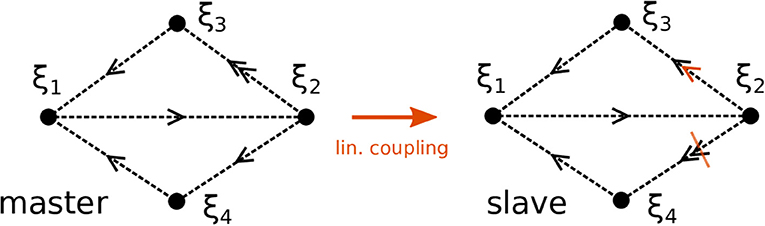
Figure 1. Topology of two Kirk-Silber networks. The networks initially differ in their expanding eigenvalues at ξ₂. Sketched in orange is the linear coupling and its effect to increase (decrease) the eigenvalues toward ξ₃ (ξ₄), respectively, in the slave system.

FIGURE 2

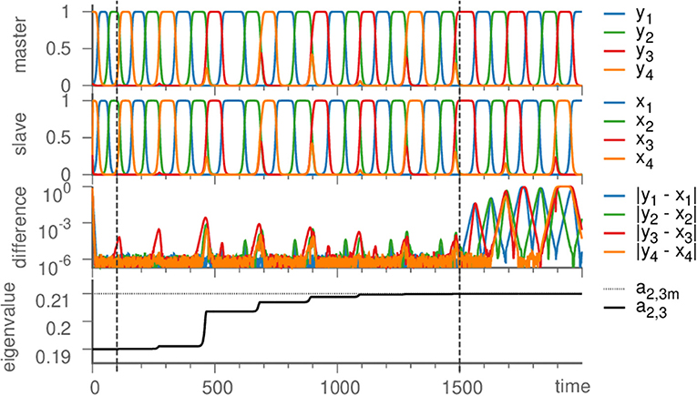
Figure 2. Learning dynamics near the Kirk-Silber network. From top to bottom: Dynamics of the master system, the slave system, their difference, and the eigenvalue a_2,3 are plotted against time. Vertical dashed lines mark the beginning of learning (t = 100) and its end (t = 1, 500), at which time also the coupling is turned off (→ ϑ = 0), so that due to different noise realizations the system states slowly diverge. Parameters are ϑ = 1, γ = 0.5, ζ = 50, σ = 10⁻⁶; eigenvalues are chosen as a_rad. = −1, a_contr. = −0.22, a_exp. = 0.2, and a_2,3m = 0.21.

3. Inferring Heteroclinic Networks With Increasing Complexity

In this section, we illustrate our method of the previous section by heteroclinic networks with increasingly complex features. As the simplest non-trivial topology we choose the Kirk-Silber network in section 3.1. At this example, we demonstrate how not only one, but all eigenvalues are recovered by the template without any prior knowledge. In addition, we point out how even the noise level may be captured by the learning method. Moreover, in section 3.2 we analyze the effect of a mismatch between the system that generated the input and the template system. Significant differences in the ODEs of the two systems strongly affect the convergence of radial eigenvalues, while the remaining eigenvalues are mostly inferred well. Furthermore, in section 3.3 we focus on larger networks with more complex topologies. We both probe our method at a highly regular, hierarchical heteroclinic network which exhibits two time scales, and construct a random heteroclinic network (by the simplex method) to generate the input and reconstruct its topology by learning. The latter example underlines the role of noise in how extensively the heteroclinic network is explored, especially in the case of an irregular topology with heterogeneous preferences of heteroclinic connections.

3.1. Inferring All Eigenvalues and the Noise Level

As the basic example in section 2, we demonstrated the successful inference of a single eigenvalue of a Kirk-Silber network. Actually, however, all eigenvalues may be inferred at the same time. Thus it is possible to start with a template with unbiased randomly or uniformly chosen parameters and infer the whole topology of a simple heteroclinic network. As demonstration, again we choose the Kirk-Silber network and initialize all eigenvalues as 0. The learning method then infers the values of the generating system, c.f. Figure 3. It is convenient to distinguish the different kinds of eigenvalues and refer to them by standard terminology [31] according to their respective eigendirection (radial, contracting, expanding, and transverse). Note that transverse eigenvalues converge only slightly slower than contracting and expanding ones, while radial eigenvalues pose a greater difficulty and converge much slower. Therefore, accelerating the learning process for radial eigenvalues (by choosing ρ ≥ 1) may be useful to moderate this effect.

FIGURE 3

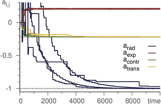
Figure 3. Learning all eigenvalues of a Kirk-Silber network. Eigenvalues are grouped by their corresponding direction. Horizontal dotted lines mark the true values. Transverse eigenvalues converge slightly slower, radial significantly. Parameters are ϑ = 5, γ = 1, ρ = 10, and σ = 10⁻⁶.

Up to this point we neglected a careful discussion of the influence of noise, although noise has to be present in the generating system to sustain the switching between saddles. If the template should reproduce this switching after the input signal is switched off, it must also be subject to noise. As the noise intensity influences the pace of switching, it ought to be the same in both systems.

To discover the original noise intensity we exploit its characteristics. If the noise is lower in the template than it was in the generating system, this has no noticeable effect. However, if it is stronger in the template, contracting eigenvalues fluctuate during learning, c.f. Figure 4. Thus, by performing multiple learning trials with decreasing σ in Equation (1), the correct noise level (as inherent in the input) may be recovered.

FIGURE 4

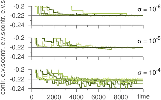
Figure 4. Influence of the noise strength on the template system during learning a Kirk-Silber network. Plotted are the contracting eigenvalues during learning. The master system has always σ = 10⁻⁶. For stronger noise in the template contracting eigenvalues fluctuate. Parameters are ϑ = 5, γ = 1, and ρ = 10.

In summary, after decoupling the template from the master system with identical dynamics, the time evolution of both systems is exactly the same if there is no noise and identical initial conditions have been used. Otherwise, i.e., under the influence of noise and depending on the initial conditions, the statistics and sequence of visited saddles in both decoupled time evolutions remain the same, but the dynamics differs in details.

3.2. Mismatched Template

In the examples above the input signal is generated by a system of ODEs that has the same form as the template. Otherwise, if the input stems from a different implementation of a simple heteroclinic network, the question arises of how this mismatch between template and generating system impacts the inference. In the following we pursue this question, as it is crucial in view of the fact that for a realistic inference task the form of the original ODEs is usually unknown.

Time continuous models of population dynamics are commonly derived as a mean-field approximation [32] of reaction equations that describe interactions at the level of individuals. One basic example of such a continuous model is the May-Leonard model [33]. It contains a heteroclinic cycle that is also known as the Busse-Heikes cycle [34], generated by the ODEs

$\begin{array}{ll}{\text{d}}_t{x}_i=x_i(1-x_i-b{x}_{i+1}-c{x}_{i+2}),& (4)\end{array}$

where 0 < c < 1 < b, b − 1 > 1 − c, and i ∈ ℤ₃ = {1, 2, 3} cyclic. The variables x_i represent population densities, thus they are restricted to the positive octant ${ℝ}_{⩾0}^3$. By a variable transformation ($x_i\to \sqrt{x_i}$) the Guckenheimer-Holmes cycle [35] emerges, which matches the form of the template. The original Busse-Heikes cycle, however, does not; it has second-order terms instead of third-order ones¹.

Nevertheless, our method is able to infer the Busse-Heikes cycle. With the default parameters (ϑ = 1, γ = 0.5, ζ = 50, and ρ = 10), we find that the radial eigenvalues fluctuate strongly, but the eigenvalues of the remaining directions converge approximately to their true values. Choosing a low value of ρ (e.g., ρ = 0.2) reduces the fluctuations of the radial eigenvalues. The resulting template follows a heteroclinic cycle with the same topology, but different shape of the approach toward the saddles, c.f. Figure 5A.

FIGURE 5

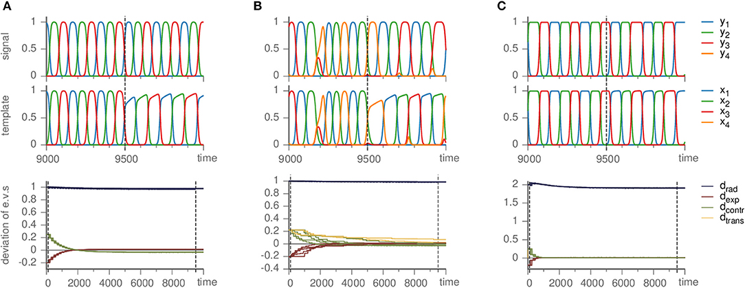
Figure 5. Effects of mismatched templates. Upper panels show the dynamics of the signal and template against time. Lower panels display the deviation of the eigenvalue in the template from their value a_i,jm in the master system, i.e., d_i,j = a_i,j − a_i,jm, sorted by the kind of direction they correspond to (radial, expanding, contracting, and transverse). Parameters are ϑ = 1, γ = 0.5. (A) Busse-Heikes cycle, with b = 1.25, c = 0.8, and ρ = 0.2. (B) Kirk-Silber network with only second-order terms, using ρ = 0.1. (C) Guckenheimer-Holmes cycle with higher order terms, using a = 1, b = 1.25, c = 0.8, α = 0.01, β = 0.01, and ρ = 1.

Since the heteroclinic cycles that we considered so far do not contain transverse directions and we want to analyze the effect of a mismatch also on the transverse eigenvalues, we modified a Kirk-Silber system in the same way (so that its terms are second-order instead of third-order). The situation is quite similar; small ρ remedies the fluctuation of radial eigenvalues, whereas the transverse eigenvalues converge toward their true values, only slower than expanding and contracting ones, c.f. Figure 5B.

One further possible mismatch of the template and the generating system is due to higher order terms. To check the effect, we modified a Guckenheimer-Holmes cycle by adding two fourth-order terms:

$\begin{array}{ll}{\text{d}}_t{x}_i=x_i(1-a{x}_i^2-b{x}_{i+1}^2-c{x}_{i+2}^2-\alpha x_i^4-\beta x_i^2{x}_{i+1}^2).& (5)\end{array}$

The additional terms do not break the ${\mathbb{Z}}_2^3$ equivariance. Thus, for |α| and |β| small, the heteroclinic cycle persists (it is structurally stable). While the second term affects the dynamics far from the saddles (for β ≠ 0), the first one acts in their vicinity. More precisely, α ≠ 0 changes the position of the saddles and also the eigenvalues, so |α| ≪ 1 is necessary to maintain the heteroclinic cycle.

As long as the cycle persists, our method correctly identifies it and approximately infers the eigenvalues (independently on whether they are original or changed due to α ≠ 0) of the generating system, c.f. Figure 5C. Here, as in the other cases of mismatched templates, the eigenvalues corresponding to radial directions fluctuate and converge to values different from the ones in the generating system. More precisely, we observed radial eigenvalues to be only slightly negative, even though these directions should be definitely stable. In contrast to section 3.1 setting ρ ≥ 1 is not helpful, but intensifies the problem. Instead, a possible remedy is to ensure that radial directions are stable by fixing the radial eigenvalues to a negative value (e.g., −1) from the beginning and keeping them at this value rather than changing them by the learning dynamics (by setting ρ = 0), see the following example.

3.3. Inferring Larger Regular and Irregular Networks

The example networks presented up to this point were rather simple in their topology, involving four saddles at most. Larger networks may pose additional challenges for inference, as we point out by the following two examples: one is a highly regular, hierarchical heteroclinic network with nine nodes; the other one is a random heteroclinic network composed of 12 nodes with heterogeneous in- and out-degrees.

In Voit and Meyer-Ortmanns [36], we constructed a heteroclinic network ${H}$ that is hierarchically structured. It consists of three small heteroclinic cycles (SHCs) that constitute the saddles of a large heteroclinic cycle (LHC). This hierarchy is produced by a difference of the expanding eigenvalues associated with connections belonging to one SHC vs. connections between different SHCs. The structural hierarchy translates to a hierarchy in time scales, which amounts to the modulation of fast oscillations by slower ones. The network ${H}$ obeys a ℤ₃ × ℤ₃ symmetry. Thus it is highly regular, as is its dynamics. All saddles are visited equally often, and all SHCs dominate with the same frequency.

We apply our inference method to the dynamics generated by the very system described in Voit and Meyer-Ortmanns [36], c.f. Figure 6. It thus deviates from the template dynamics by containing only second-order terms compared to the third-order terms of the template. This mismatch leads to a deviation of the inferred radial eigenvalues from the real ones, c.f. Figure 6D, just as expected from the previous section. Nevertheless, the topology of ${H}$ and its structural hierarchy (manifest as the difference between the two kinds of expanding eigenvalues in the small and large heteroclinic cycles) is inferred correctly. The resulting dynamics of the template thus reproduces the same sequence of saddles visited as the original system. Frequency and amplitude, however, are not recovered accurately.

FIGURE 6

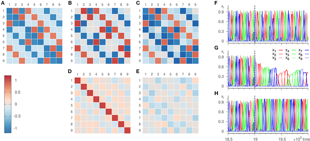
Figure 6. Eigenvalues a_i,j and dynamics of the hierarchical heteroclinic network ${H}$. Panel (A) depicts the original values, (B) the values inferred with parameters ϑ = 10, γ = 20, ρ = 0.001, σ = 10⁻⁶ where a_i,j = 0 initially, and (C) the values inferred with parameters ϑ = 10, γ = 20, ρ = 0, σ = 10⁻⁶ with a_i,j = −δ_ij initially. The inference was realized over 19 × 10³ time units. The lower panels show the error of the inference, i.e., (D) the difference of panels (B,A), (E) the difference of panels (C,A). The remaining panels display the dynamics at the end of the inference process plotted against time. Panel (F) shows the input signal, (G,H) the dynamics of the templates that resulted in (B,C), respectively.

As an alternative, we fixed the radial eigenvalues to their true value a_i,i = −1 and subjected only a_i,j for i ≠ j to the learning method (setting ρ = 0). For these entries, the error of the inference is comparable to the previous situation, c.f. Figure 6E. In addition, due to employing the true radial eigenvalues, the resulting dynamics does not only reproduce the sequence of the visited saddles correctly, but also recovers the frequency and amplitude of the oscillations to a good agreement, c.f. Figure 6H.

For the random heteroclinic network, we generated a 12 node Erdős–Rényi graph with edge probability 0.2, without self-loops. Subsequently, two-loops were removed by deleting one of the edges each, whilst ensuring that the in- and out-degree at all nodes is at least one. Figure 7 depicts the topology of the resulting graph ${G}$.

FIGURE 7

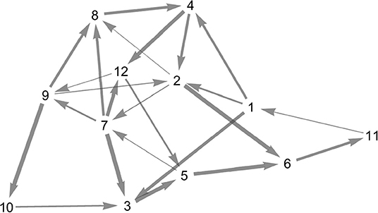
Figure 7. Topology of the random heteroclinic network ${G}$. The edge thickness is determined by the magnitude of the expanding eigenvalue at the node from which the respective heteroclinic orbit originates.

From the graph we generated the heteroclinic network by employing the same form of ODEs as in the template Equation (1) and choosing the eigenvalues a_i,j from the adjacency matrix A in the following way:

$\begin{array}{ll}{a}_{i,j}=\{\begin{array}{ll}X\in (0.4,0.6)\hfill & \text{for }{A}_{i,j}=1\hfill \\ X\in (-1.1,-0.9)\hfill & \text{for }{A}_{i,j}=0\hfill \end{array}& (6)\end{array}$

with X a random variable taken uniformly from the specified interval. The choice of these intervals is arbitrary to some extent. Mainly, eigenvalues in expanding directions (A_i,j = 1) must be positive, while contracting, radial and transverse eigenvalues must be negative. Furthermore, for the heteroclinic network as a whole to be attractive, “contraction must surpass expansion”. The size of the intervals controls the degree of heterogeneity in the preference of heteroclinic orbits. Overall, this process is thus an adapted version of the simplex method [19], which describes how to construct a simple heteroclinic network for a given graph.

For our choice of intervals, the expanding eigenvalues differ sufficiently, so that the system dwells more frequently in some parts of the network than in others. The relevance of this becomes especially clear once the learning method is applied. Strong noise is required to infer all parts of the heteroclinic network, c.f. Figure 8. Then, however, also the inferred eigenvalues fluctuate strongly. For low noise levels, on the other hand, some saddles are visited only rarely. For example, saddle 10 is not visited at all for σ = 10⁻⁵, but 12 times for σ = 0.002, c.f. Figure 8F. This scarcity of visits to certain saddles is one factor that may lead to a comparatively bad inference of their eigenvalues, c.f. Figure 8E. However, other factors such as the topology of the heteroclinic network and the recent history of the trajectory before arriving at a certain saddle play a role as well.

FIGURE 8

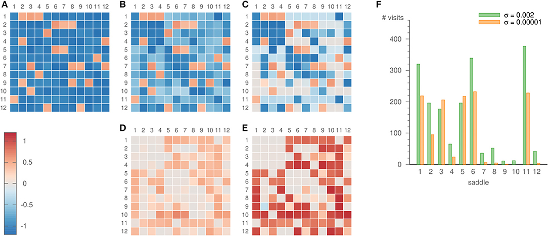
Figure 8. Eigenvalues a_i,j of the random heteroclinic network ${G}$. Panel (A) depicts the original values, (B) the values inferred with parameters ϑ = 5, γ = 3, ρ = 0.2, σ = 0.002, and (C) the values inferred with parameters ϑ = 5, γ = 3, ρ = 0.2, σ = 0.00001. The inference was realized over 19 × 10³ time units. The lower panels show the error of the inference, i.e., (D) the difference of panels (B,A), (E) the difference of panels (C,A). Panel (F) displays the number of times the dynamics visits each of the saddles for both noise strengths.

For practical applications the obvious trade-off between exploring the whole network (high noise level) and the quality of the inferred eigenvalues (low noise level) is of minor importance. Indeed, for weak noise it would be impossible to infer some of the saddles, but the actual dynamics neither visits these saddles.

Besides the noise strength, the length of the input signal needs to be taken into account. Longer input is beneficial, as weakly attached parts of the networks get visited more often. If the input is too short, only the most probable cycles of the heteroclinic network become inferred. For example, running the inference for merely 1500 time units, we observed the resulting heteroclinic network settle to the cycles 1 → 2 → 6 → 11 → 1, or 1 → 3 → 5 → 6 → 11 → 1.

4. Discussion

In summary, we have introduced a novel method of learning simple heteroclinic networks. It is based on an unbiased template system of a heteroclinic network in combination with a learning dynamics that progressively alters the eigenvalues at the saddles. The system thereby dynamically infers the eigenvalues at all saddles and thus reconstructs the topology of the heteroclinic network that generated the signal. A key ingredient is the linear coupling to the input signal, which forces the dynamics of the input onto the template. Only this enables the learning, which primarily takes place when the system visits the saddle equilibria. The trained template then reproduces sequences of metastable states most similar to the input time series.

We worked out the performance of this method for various examples, inferring all eigenvalues even in comparatively large heteroclinic networks. Moreover, we illustrated possible difficulties that the noise level or a mismatch of template and generating system can pose, for example. We pointed out strategies to handle them. A subtle point will be to achieve a deeper understanding of what determines the speed of learning the eigenvalues of saddles, that is, its dependence on the topology of the heteroclinic network, the noise level and other factors.

In view of engineering underlying heteroclinic networks from a given data set, our method provides a continuous counterpart to designing simple finite-state machines from given example data, as it automatically interpolates between subsequent maxima. If data of sequential switching between different metastable states suggest games of winnerless competition behind their generation, it would be natural to attempt a learning of rates at a first place (say in generalized Lotka-Volterra models), rather than a learning of eigenvalues. In simple heteroclinic networks it is the local information stored in the eigenvalues of the saddles that is sufficient to control and learn the time evolution of the dynamics in a desired way, bridging the global (non-local) distance between the different saddles. Therefore, as long as the assumed heteroclinic network is simple, one would learn the rates as a function of the learned eigenvalues, while the eigenvalues at the saddles are expressed in terms of the rates.

Simple heteroclinic networks are specific in the sense that the saddles lie on the coordinate axes, the phase space has a dimension that is given by the number of saddles, and together with the imposed symmetry one knows from the local information of the eigenvalues at one saddle at which saddle one ends up next. It is therefore sufficient to learn the eigenvalues (and thus mimic the local dynamics) in order to reproduce the global dynamics. In general (and in particular in the context of heteroclinic computing), the heteroclinic networks are non-simple and the dimension of phase space is lower than the number of saddles. It is an interesting open challenge to derive rules for learning non-simple heteroclinic networks and possibly combine these with the concept of heteroclinic computing.

Data Availability Statement

All datasets generated for this study are included in the article/supplementary material.

Author Contributions

MV and HM-O designed the study, discussed the results, and contributed to editing the manuscript. MV conducted numerical simulations, carried out the analysis, and prepared the manuscript. HM-O supervised the study.

Funding

Funding by the German Research Foundation (DFG, contract ME-1332/28-1) and by Jacobs University Bremen is gratefully acknowledged.

Conflict of Interest

The authors declare that the research was conducted in the absence of any commercial or financial relationships that could be construed as a potential conflict of interest.

Acknowledgments

We thank Ulrich Parlitz for helpful discussions during his visit at Jacobs University Bremen in summer 2019.

Footnotes

1. ^Commonly, the terms “Busse-Heikes cycle” and “Guckenheimer-Holmes cycle” are used synonymously, as the heteroclinic cycles (as objects in phase space) are diffeomorphic to each other. In this article, however, we specifically distinguish the two different ODE systems by these terms.

References

1. Krupa M. Robust Heteroclinic Cycles. J Nonlinear Sci. (1997) 7:129–76. doi: 10.1007/BF02677976

CrossRef Full Text | Google Scholar

2. Kori H, Kuramoto Y. Slow switching in globally coupled oscillators: robustness and occurrence through delayed coupling. Phys Rev E. (2001) 63:046214. doi: 10.1103/PhysRevE.63.046214

PubMed Abstract | CrossRef Full Text | Google Scholar

3. Wordsworth J, Ashwin P. Spatiotemporal coding of inputs for a system of globally coupled phase oscillators. Phys Rev E. (2008) 78:066203. doi: 10.1103/PhysRevE.78.066203

PubMed Abstract | CrossRef Full Text | Google Scholar

4. Schittler Neves F, Timme M. Computation by switching in complex networks of states. Phys Rev Lett. (2012) 109:018701. doi: 10.1103/PhysRevLett.109.018701

PubMed Abstract | CrossRef Full Text | Google Scholar

5. Afraimovich V, Tristan I, Huerta R, Rabinovich MI. Winnerless competition principle and prediction of the transient dynamics in a Lotka–Volterra model. Chaos Interdiscip J Nonlinear Sci. (2008) 18:043103. doi: 10.1063/1.2991108

PubMed Abstract | CrossRef Full Text | Google Scholar

6. Hauert C, Szabó G. Game theory and physics. Am J Phys. (2005) 73:405–14. doi: 10.1119/1.1848514

CrossRef Full Text | Google Scholar

7. Szabó G, Vukov J, Szolnoki A. Phase diagrams for an evolutionary prisoner's dilemma game on two-dimensional lattices. Phys Rev E. (2005) 72:047107. doi: 10.1103/PhysRevE.72.047107

PubMed Abstract | CrossRef Full Text | Google Scholar

8. Nowak MA, Sigmund K. Biodiversity: bacterial game dynamics. Nature. (2002) 418:138–9. doi: 10.1038/418138a

CrossRef Full Text | Google Scholar

9. Rabinovich MI, Afraimovich VS, Varona P. Heteroclinic binding. Dyn Syst. (2010) 25:433–42. doi: 10.1080/14689367.2010.515396

CrossRef Full Text | Google Scholar

10. Rabinovich MI, Varona P, Tristan I, Afraimovich VS. Chunking dynamics: heteroclinics in mind. Front Comput Neurosci. (2014) 8:22. doi: 10.3389/fncom.2014.00022

PubMed Abstract | CrossRef Full Text | Google Scholar

11. Rabinovich MI, Huerta R, Varona P, Afraimovich VS. Transient cognitive dynamics, metastability, and decision making. PLoS Comput Biol. (2008) 4:e1000072. doi: 10.1371/journal.pcbi.1000072

PubMed Abstract | CrossRef Full Text | Google Scholar

12. Komarov MA, Osipov GV, Suykens JAK. Metastable states and transient activity in ensembles of excitatory and inhibitory elements. EPL Europhys Lett. (2010) 91:20006. doi: 10.1209/0295-5075/91/20006

CrossRef Full Text | Google Scholar

13. Fingelkurts A, Fingelkurts A. Information flow in the brain: ordered sequences of metastable states. Information. (2017) 8:22. doi: 10.3390/info8010022

CrossRef Full Text | Google Scholar

14. Afraimovich VS, Rabinovich MI, Varona P. Heteroclinic contours in neural ensembles and the winnerless competition principle. Int J Bifurc Chaos. (2004) 14:1195–208. doi: 10.1142/S0218127404009806

CrossRef Full Text | Google Scholar

15. Michel CM, Koenig T. EEG microstates as a tool for studying the temporal dynamics of whole-brain neuronal networks: a review. NeuroImage. (2018) 180:577–93. doi: 10.1016/j.neuroimage.2017.11.062

PubMed Abstract | CrossRef Full Text | Google Scholar

16. Nehaniv CL, Antonova E. Simulating and reconstructing neurodynamics with Epsilon-automata applied to electroencephalography (EEG) microstate sequences. In: 2017 IEEE Symposium Series on Computational Intelligence (SSCI). Honolulu, HI (2017). p. 1–9. doi: 10.1109/SSCI.2017.8285438

CrossRef Full Text | Google Scholar

17. Creaser J, Ashwin P, Postlethwaite C, Britz J. Noisy network attractor models for transitions between EEG microstates. arXiv:1903.05590 (2019).

Google Scholar

18. Van De Ville D, Britz J, Michel CM. EEG microstate sequences in healthy humans at rest reveal scale-free dynamics. Proc Natl Acad Sci USA. (2010) 107:18179–84. doi: 10.1073/pnas.1007841107

PubMed Abstract | CrossRef Full Text | Google Scholar

19. Ashwin P, Postlethwaite C. On designing heteroclinic networks from graphs. Phys Nonlinear Phenom. (2013) 265:26–39. doi: 10.1016/j.physd.2013.09.006

CrossRef Full Text | Google Scholar

20. Field MJ. Heteroclinic networks in homogeneous and heterogeneous identical cell systems. J Nonlinear Sci. (2015) 25:779–813. doi: 10.1007/s00332-015-9241-1

CrossRef Full Text | Google Scholar

21. Ashwin P, Postlethwaite C. Designing heteroclinic and excitable networks in phase space using two populations of coupled cells. J Nonlinear Sci. (2016) 26:345–64. doi: 10.1007/s00332-015-9277-2

CrossRef Full Text | Google Scholar

22. Horchler AD, Daltorio KA, Chiel HJ, Quinn RD. Designing responsive pattern generators: stable heteroclinic channel cycles for modeling and control. Bioinspir Biomim. (2015) 10:026001. doi: 10.1088/1748-3190/10/2/026001

PubMed Abstract | CrossRef Full Text | Google Scholar

23. Selskii A, Makarov VA. Synchronization of heteroclinic circuits through learning in coupled neural networks. Regul Chaot Dyn. (2016) 21:97–106. doi: 10.1134/S1560354716010056

CrossRef Full Text | Google Scholar

24. Calvo Tapia C, Tyukin IY, Makarov VA. Fast social-like learning of complex behaviors based on motor motifs. Phys Rev E. (2018) 97:052308. doi: 10.1103/PhysRevE.97.052308

PubMed Abstract | CrossRef Full Text | Google Scholar

25. Seliger P, Tsimring LS, Rabinovich MI. Dynamics-based sequential memory: winnerless competition of patterns. Phys Rev E. (2003) 67:011905. doi: 10.1103/PhysRevE.67.011905

PubMed Abstract | CrossRef Full Text | Google Scholar

26. Krupa M, Melbourne I. Asymptotic stability of heteroclinic cycles in systems with symmetry. II. Proc R Soc Edinb Sect Math. (2004) 134:1177–97. doi: 10.1017/S0308210500003693

CrossRef Full Text | Google Scholar

27. Hofbauer J, Sigmund K. Evolutionary Games and Population Dynamics. Cambridge: Cambridge University Press (1998).

Google Scholar

28. Hoyle R. Pattern Formation: An Introduction to Methods. Cambridge: Cambridge University Press (2006).

Google Scholar

29. Pecora LM, Carroll TL. Master stability functions for synchronized coupled systems. Phys Rev Lett. (1998) 80:4. doi: 10.1103/PhysRevLett.80.2109

CrossRef Full Text | Google Scholar

30. Kirk V, Silber M. A competition between heteroclinic Cycles. Nonlinearity. (1994) 7:1605–21. doi: 10.1088/0951-7715/7/6/005

CrossRef Full Text | Google Scholar

31. Krupa M, Melbourne I. Asymptotic stability of heteroclinic cycles in systems with symmetry. Ergod Theory Dyn Syst. (1995) 15:121–47. doi: 10.1017/S0143385700008270

CrossRef Full Text | Google Scholar

32. Van Kampen NG. Stochastic Processes in Physics and Chemistry. Amsterdam: Elsevier (1992).

Google Scholar

33. May RM, Leonard WJ. Nonlinear aspects of competition between three species. SIAM J Appl Math. (1975) 29:243–53. doi: 10.1137/0129022

CrossRef Full Text | Google Scholar

34. Busse FH, Heikes KE. Convection in a rotating layer: a simple case of turbulence. Science. (1980) 208:173–5. doi: 10.1126/science.208.4440.173

PubMed Abstract | CrossRef Full Text | Google Scholar

35. Guckenheimer J, Holmes P. Structurally stable heteroclinic cycles. Math Proc Camb Philos Soc. (1988) 103:189–92. doi: 10.1017/S0305004100064732

CrossRef Full Text | Google Scholar

36. Voit M, Meyer-Ortmanns H. A hierarchical heteroclinic network: controlling the time evolution along its paths. EPJ ST. (2018) 227:1101–15. doi: 10.1140/epjst/e2018-800040-x

CrossRef Full Text | Google Scholar