A Phase Field Approach to Trabecular Bone Remodeling

1. Introduction

Bone undergoes a continuous renewal process, which helps to maintain its mechanical performance and allows for adaptation to changes in mechanical requirements. Different cells are involved in this remodeling process: osteoclasts, which resorb bone, and osteoblasts, which deposit bone. The process is controlled by mechanosensing osteocytes [1–4] and provides an example of a homeostatic system where external mechanical loads control the bone mass and structure. Various experimental and theoretical studies analyze the remodeling process on different levels of detail [5–9]. We here introduce a continuous modeling approach with the potential to combine different scales in an efficient way. In an abstract setting we consider bone as a shape changing structure, with concentrations of mechanosensing cells within the bone and resorbing and depositing cells on the bone surface. Depending on the surface concentrations the structure is adapted. In contrast to previous modeling approaches, using micro finite element analysis [10–14], we describe the structure implicitly using a time-dependent phase field function. This not only leads to a more accurate model, as the artificial voxel-roughness of the bone surface can be avoided, but also to a drastic reduction of system size and required computing time. Phase field models have been developed to describe shape changing structures, e.g., in solidification [15] or multiphase fluids [16]. In the last decade these models were extended to be used as a general numerical tool to solve problems in complex time-evolving geometries [17] and have since been established for two-phase flow [18–21], biomembranes [22, 23], single cell mechanics [24], and fluid-structure interaction [25].

In the context of bone, phase field models have been used to compute the mechanical properties of trabecular bone structures [26] and have been validated against micro finite element analysis. The required implicit description of the bone structure can be obtained from imaging tools, such as μCT and μMR by standard algorithms. From the voxel representation of the segmented image a smooth surface triangulation can be constructed, from which a signed distance function and the initial phase field function can be computed. The computation of the remodeling process can then be done on a simple cubic domain, which can easily be decomposed for efficient parallel computations. Figure 1 shows an example of an implicitly described trabecular structure, the phase field representation and details of the phase field function.

FIGURE 1

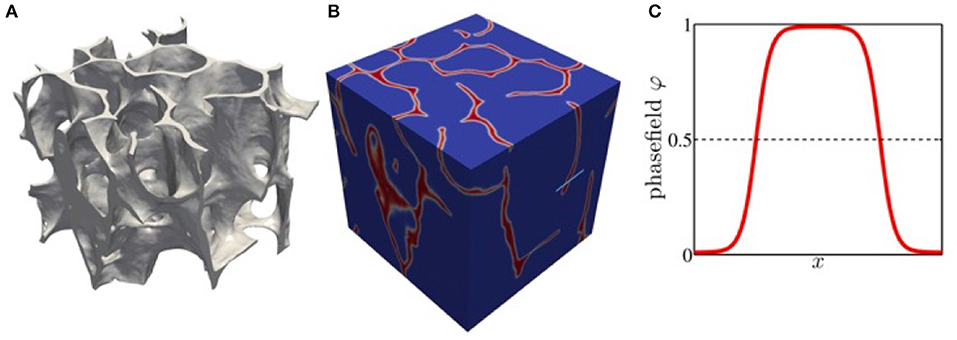
Figure 1. (A) Trabecular structure from sheep tomography data represented by level surface of the phase field function. (B) phase field function in a box domain. (C) phase field function along the light blue line in (B) with ϕ = 1 representing the bone structure.

The paper is organized as follows: In section 2, we review the current understanding of the bone remodeling process and motivate approximations for our computational approach. Our goal is to introduce a minimal model to demonstrate the potential of the phase field modeling and to point out possible model extensions. We also compare our assumptions with existing micro finite element analysis. In section 3, we propose our mathematical model, the numerical approach and required preprocessing steps and provide details on the μCT data. In section 4, we describe results which relate the bone morphology to an applied force. In section 5, we discuss the results and give conclusions.

2. Materials and Methods

We briefly review the role of the different cells which are involved in the remodeling process and describe the mechanical properties of bone on the level required for our continuous modeling approach.

2.1. Osteocytes

Osteocytes form a network throughout the bone matrix by connecting with each other and the lining cells on the bone surface. They sense mechanical loads and transduce the mechanical signal into a chemical response, which is realized by signaling molecules. On the bone surface these molecules orchestrate the recruitment and activity of osteoblasts and osteoclasts, resulting in the adaptation of bone mass and structure. How the osteocytes sense the mechanical loads and coordinate adaptive alterations in bone mass and architecture is not yet completely understood. For a current review see Klein-Nulend et al. [27]. For the mechanical sensing several mechanisms have been proposed [28]. Within our modeling approach we consider the volumetric compression and the strain energy density as two options to stimulate the osteocytes. The signaling molecules in the bone are then modeled through a diffusion process, with a decay rate and the mechanical stimulus as a source term. This differs from typical micro finite element analysis approaches, where an exponential decay of the signal molecules is assumed and only contributions within a certain distance are accounted for, e.g., Huiskes et al., [4] and Ruimerman et al., [7].

2.2. Osteoblasts and Osteoclasts

A large number of hypotheses have been postulated regarding bone-cell communication and the role played by various receptor-ligand pathways. Various modeling approaches are concerned with the biochemical signaling between active osteoclasts and osteoblasts [29–31]. However, they all work on spatial averages and are not yet incorporated in a computational bone remodeling process. We therefore here only use an effective modeling approach by directly considering the concentration of the signaling molecules at the bone surface as an indicator for resorption and deposition. Similar approximations are made in typical micro finite element analysis approaches with various functional forms. The influences of different remodeling rules like linear, step functions or the originally proposed profile by Frost [32] with a lazy zone have been compared in Dunlop et al. [5]. While the exact form of the remodeling rule is of importance for quantitative predictions, all forms lead to the emergence of trabecular-like patterns.

2.3. Trabecular Bone Structure and Mechanical Behavior

Also from a mechanical perspective, trabecular bone is a highly complex material, being anisotropic with different strengths in tension, compression, and shear and with mechanical properties that vary widely across anatomic sites, and with aging and disease [33]. Various of these material properties remain uncertain. However, different experiments have shown a linear behavior [34] and also have related the anisotropy of the mechanical properties to the bone structure [35]. We therefore also for this part of the model consider the simplest possible approach, an isotropic material with prescribed elastic modulus and Poisson ratio but resolve the trabecular bone structure. The same approximations are made in most micro finite element analysis approaches [36–38].

3. Theory

3.1. Mathematical Model

Let Ω_bone be the bone structure and Ω a cuboid computational domain of size L = (L_x, L_y, L_z) such that Ω_bone ⊂ Ω. The mechanical material properties of the trabeculae are supposed to be isotropic with Young's modulus E and Poisson's ratio ν. The bone deformation is described by the displacement vector u obeying the partial differential equation [39]

$\begin{array}{ll}\nabla ·\sigma =0\text{ in }{\Omega }_{\text{bone}},& (1)\end{array}$

with the linear elastic stress tensor [39]

$\begin{array}{ll}\sigma =\mu (\nabla \text{u}+\nabla {\text{u}}^T)+\lambda I\nabla ·\text{u},& (2)\end{array}$

where I is the identity matrix and μ, λ are the Lame coefficients

$\begin{array}{l}\mu =\frac{E}{2(1+\nu )},\lambda =\frac{E\nu }{(1+\nu )(1-2\nu )}.\end{array}$

Compression is achieved by applying Dirichlet boundary conditions to the normal component of u on ∂Ω, such that u_{x, y, z} = 0 if x, y, z = 0 and u_{x, y, z} = ū_{x, y, z} if x = L_x, y = L_y, z = L_z, while the tangential displacement components are free and ū_{x, y, z} are adapted such that the normal forces (F_x, F_y, F_z) are kept constant. At the remaining boundaries ∂Ω_bone we assume no outer forces and set σ·n = 0, where n is the normal to Ω_bone.

We assume that osteocytes are continuously distributed through Ω_bone and that a growth stimulating signal is produced in the osteocytes stimulated by either the volumetric compression or the strain energy density

$\begin{array}{lll}{S}_{\text{vc}}=|\nabla ·\text{u}|& \left(\text{volumetric compression}\right),& (3)\end{array}$

$\begin{array}{lll}{S}_{\text{sed}}=\frac{1}{4}\sigma :(\nabla \text{u}+\nabla {\text{u}}^T)& \left(\text{strain energy density}\right).& (4)\end{array}$

The signal is propagated by a diffusive process with a constant decay rate. Denoting the concentration of the signaling molecule by c, this leads to the equation

$\begin{array}{lll}kc-d\Delta c=S& \text{ in }{\Omega }_{\text{bone}},& (5)\end{array}$

with boundary condition n·∇c = 0 on ∂Ω_bone, where k is the decay rate and d the diffusion coefficient, both assumed to be constant and S = S_{vc, sed}. Due to the different time scale, if compared with the remodeling process, we consider the stationary solution.

Finally growth is triggered directly according to the concentration c at the trabecular surface. We assume that the growth velocity in normal direction V = V_{lin, lazy} depends linearly on the signal strength, without or with a lazy zone [14]

$\begin{array}{lll}{V}_{\text{lin}}=\alpha c-\beta & \text{ on }\partial {\Omega }_{\text{bone}},& (6)\end{array}$

$\begin{array}{lll}{V}_{\text{lazy}}=\alpha (c-min(T,max(-T,c-1)))-\beta & \text{on }\partial {\Omega }_{\text{bone}},& (7)\end{array}$

with positive constants α and β and an intermediate range for c where no growth occurs, controlled by the threshold value T.

Mathematically the resulting system of Equations (1)–(7) is a free boundary problem. According to the proposed normal forces (F_x, F_y, F_z) on δΩ the displacement u and the concentration c have to be computed in Ω_bone. The obtained signal c at δΩ_bone is then used to update the time dependent bone structure Ω_bone. This non-linear problem has to be iterated until the solution for u, c, and Ω_bone converge.

3.2. Numerical Solution

In micro finite element analysis the time dependent bone structure is accounted for by adding and removing voxels to Ω_bone. This is not only costly as it requires a high spatial resolution, it also leads to an artificial roughness of the bone surface. Various numerical methods have been proposed to avoid such manipulation of the computational domain. One of the most successful approaches is the phase field or diffuse domain approach [17]. Here Ω_bone is described implicitly through a smooth phase field function $\varphi =0.5(1-tanh(r/(\sqrt{8}ϵ)))$ in Ω, with a small parameter ϵ determining the width of the diffuse interface and the signed distance function r, with r = 0 at δΩ_bone, r > 0 in Ω_bone and r < 0 in Ω\Ω_bone. For ϵ → 0, ϕ converges to the characteristic function for Ω_bone. Using ϕ we can now reformulate the problem in the time-independent domain Ω. The diffuse domain approximation of Equations (1) and (2) reads

$\begin{array}{ll}\mu \nabla ·\left[\varphi (\nabla \text{u}+\nabla {\text{u}}^T)\right]+\lambda \nabla \left[\varphi \nabla ·\text{u}\right]=0\text{ in }\Omega .& (8)\end{array}$

The boundary condition σ·n = 0 is implicitly included (see Aland et al., [26]). Applying the same approach from Li et al. [17] to Equation (5) we obtain

$\begin{array}{ll}k\varphi c-d\nabla ·(\varphi \nabla c)=\varphi S\text{ in }\Omega ,& (9)\end{array}$

which also already includes the boundary condition n·∇c = 0. Adapting the bone domain with normal velocity V can be realized by solving

$\begin{array}{l}{\partial }_t\varphi +V|\nabla \varphi |=\gamma (-{\varphi }^3+1.5{\varphi }^2-0.5\varphi )\\ +\gamma {ϵ}^2\frac{\nabla {\varphi }^T·\nabla \nabla \varphi ·\nabla \varphi }{|\nabla \varphi {|}^2}\text{ in }\Omega ,& (10)\end{array}$

with a mobility factor γ (see Folch et al., [40]). The terms on the right hand side essentially guarantee the tanh-profile of ϕ and the left hand side models the transport of ϕ by V. Using matched asymptotic analysis one can show (see Li et al. [17]), that the system of Equations (8)–(10) converge for ϵ → 0 to the original problem (1)–(5) with the boundary moved with velocity V and boundary conditions σ·n = 0 and ∇c·n = 0. We can now use standard discretization techniques to solve for u, c, and ϕ in Ω, again iteratively until the system converges.

For a computationally efficient treatment adaptive mesh refinement is used. A high resolution within the diffuse interface is required, which needs to be of order ϵ and is comparable to the initial voxel scale. However, away from the diffuse interface a coarser mesh can be used, which drastically reduces the computational cost. The efficiency can further be improved by using differently refined meshes for the components [41, 42]. We here use a parallel adaptive finite element approach on unstructured meshes which is implemented in the open source toolbox AMDiS [43, 44].

3.3. Preprocessing

To use the phase field approach for real bone structures requires various preprocessing steps. From the segmented data on the voxel scale, first a surface triangulation is constructed, from which in a second step the signed distance and phase field function can be computed. Figure 2 shows the three steps. Various approaches are available for achieving these steps. We here use ParaView (http://www.paraview.org) for the generation and smoothing of the surface mesh. Mesh generation has become a standard tool. However, the quality of these meshes in terms of regularity is often very poor. Automatic construction of high quality surface meshes is still not possible for arbitrary surfaces and is an ongoing research topic. The available algorithms in ParaView provide a reasonable compromise between usability and mesh quality. To compute the signed distance function we embed the structure in a cube and adaptively refine the mesh until we obtain the proposed accuracy to resolve the surface. For each node we compute the shortest distance to the surface using raytracing. The approach is implemented in MeshConv (https://gitlab.math.tu-dresden.de/wir/meshconv) and produces the initial mesh and signed distance function for the computation in AMDiS (https://gitlab.math.tu-dresden.de/wir/amdis). All these software tools are available under an open source license.

FIGURE 2

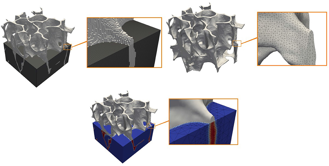
Figure 2. Cuboidal segment of a sheep bone. From top left to bottom right: Segmented voxel representation (bone in light gray), triangulated smooth surface representation and phase field description with smooth level surface and adapted volume triangulation.

3.4. Validation

Before we simulate bone remodeling on real bone structures, we consider two simple examples, a cylinder and a cross, for which we compare the results with a micro finite element analysis approach [4, 7], and in the cylinder case also with a semi-analytical solution. We consider both types of stimuli, the volumetric compression and the strain energy density and consider the linear growth law Equation (6).

For a cylinder with radius R and a compression force F_z, we obtain for the stimuli $S_{\mathrm{\text{vc}}}=(1-2\nu )\frac{F_z}{E}\frac{1}{\pi R^2}$ and $S_{\mathrm{\text{sed}}}=\frac{1}{2}\frac{F_z^2}{E}\frac{1}{{\pi }^2{R}^4}$. Both are constant in Ω_bone, which allows to solve Equation (5). We obtain $c=\frac{S}{k}$ and thus from Equation (6) the growth law $V_{\mathrm{\text{lin}}}=\frac{\alpha }{k}S-\beta$ from which the evolution of the cylinder can be obtained.

The micro finite element analysis is based on Huiskes et al. [4] and Ruimerman et al. [7]. The domain Ω is divided into a regular voxel mesh with mesh size h. Each voxel has a continuous value g ∈ [0, 1], where bone is associated with g = 1 and bone marrow corresponds to g = 0. Transient states correspond to voxels which are partly bone. The elastic modulus for a voxel and the stimuli are defined as gE and gS, respectively. The Poisson ratio remains independent of g. Instead of directly solving for the normal velocity V we first compute the change rate of a voxel's g value at ∂Ω_bone and the neighboring marrow voxels by solving ∂_tg = αc − β and restricting g ∈ [0, 1]. The normal velocity then follows by multiplying the change rate with the voxel size V = h ∂_tg and applying corrections for the lattice anisotropy. For the numerical solution of Equations (1) and (5), each voxel with g = 1 is converted to a hex-8 brick element and the resulting systems are solved by standard finite element analysis.

For the comparison we only consider non-dimensional values. The computational domain is the unit cube with L_x = L_y = L_z = 1. The voxel size, as well as the minimum grid spacing in the phase field approach is set to h = 1/128. Time steps were chosen adaptively. Other parameters are d = 1, k = 1/2, F_z = 1 for the cylinder and F_x = F_y = F_z = 1 for the cross, as well as β = 1. The parameter α is chosen depending on the considered stimulus such that the same stationary states are obtained: α_sed = 0.36 and α_vc = 0.9 for the growth experiment and α_sed = 0.04 and α_vc = 0.3 for the shrinkage simulations. These parameters lead to a stationary state with $R=\sqrt{0.6/\pi }$ and $R=\sqrt{0.2/\pi }$ for growth and shrinkage, respectively. As initial condition we thus use the opposed value, i.e., $R=\sqrt{0.2/\pi }$ (growth), $R=\sqrt{0.6/\pi }$ (shrinkage). For the simulation of a single growing cross, α_vc = 0.0919 is used and the initial radius on each side is set to $R=\sqrt{0.02/\pi }$. The remaining parameters for the phase field approach are ϵ = 0.005 and γ = 10.

In all these cases the solution of the free boundary problem converge to a stationary solution providing the adapted bone morphology to the applied force (see Figures 3–5). The results are in excellent agreement with the micro finite element results and the analytic solution, where available.

FIGURE 3

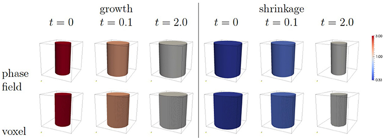
Figure 3. Cylinder growth (left) and shrinkage (right). The images correspond to the use of the volumetric compression as stimulus. The color coding corresponds to the scaled concentration αc.

FIGURE 4

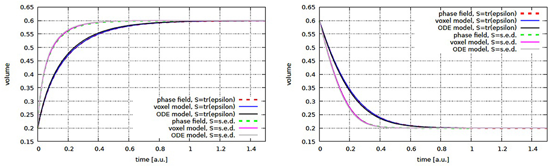
Figure 4. Cylinder volume over time for growth (left) and shrinkage (right) for volumetric compression and strain energy density as stimulus. Shown are the phase field and micro finite element results together with the semi-analytic solution (ODE model).

FIGURE 5

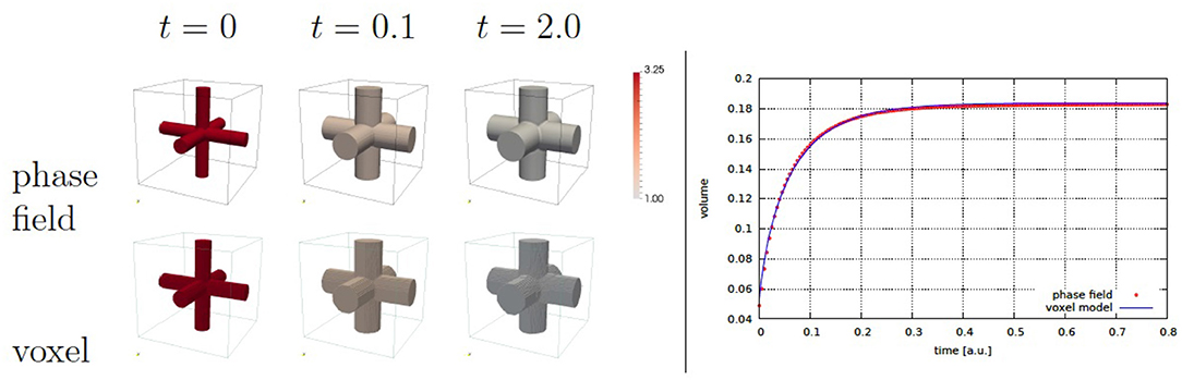
Figure 5. Cross growth evolution (left) and cross volume over time (right). The volumetric compression is used as stimulus. The color coding corresponds to the scaled concentration αc, where αc = 1 indicates the approached stationary state.

4. Results

We now apply our model to a segment of a trabecular bone, which is obtained from tomography data of a sheep vertebra. This data has been previously generated in the German Transregional Collaborative Research Centre SFB/TRR 79 and is reused for our computational study. The elastic properties are chosen as E = 6.829GPa and ν = 0.33 (see Ruimerman et al., [7], Mueller et al., [45] and Müller et al., [46]). The cubic region Ω is defined by L_x = L_y = L_z = 2.84mm. To account for the dominant loading in z-direction in the animal, the applied force is set twice as high as in the other directions F_x = F_y = 8N and F_z = 16N. The range of these forces is chosen to yield strains close to experimental observations [47]. Instead of the linear growth law used for validation we consider Equation (7) with a lazy zone determined by T = 0.2. Volumetric compression was chosen as stimulus and parameters were set to ϵ = 0.003, γ = 10. Realistic values for the remaining parameters are not clear, we hence choose values in a range that illustrates the potential of the method to simulate remodeling of the bone material: k = 1, d = 0.01, α = 690, β = 1. The computations are done in parallel on 24 cores with approximately 7.5 Mio degrees of freedom in each time step. The computational time for each setting was approximately 1 h.

Figure 6 shows the evolution obtained with these parameters. The evolution is shown up to a state for which the main morphological changes have been completed and the concentration c has been mainly equilibrated. A change in morphology is hardly visible, however the computed average microstrain in Ω_bone, $\sqrt{<\left|{ϵ}_{zz}\right|>}=2004$, with ϵ = 0.5(∇u + (∇u)^T) agrees well with physiological strains measured in bone [47].

FIGURE 6

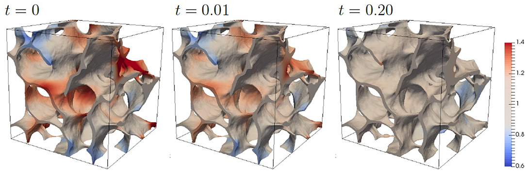
Figure 6. Evolution of bone morphology with standard parameters. The color coding corresponds to the scaled concentration αc.

To highlight the morphological adaption to anisotropic forces we consider compression forces which are increased by a factor 4 in one direction. Figure 7 shows the results. The stronger force leads to larger values for c and the adaption of the morphology strongly depending on the direction of the increased force. The change in morphology is clearly visible with regions which are formed and regions which are resorbed. The dependency of the morphology on the direction of the increased force is highlighted in Figure 8, which shows slices of the bone morphology along the xy-, xz-, and yz-plane, through the center of the domain. This visualization clearly shows that structures grow in the direction of the enhanced (four-fold) force and thus provide a proof of consistency of the modeling approach. Further validation would require in vivo μCT data of the trabecular bone segment and a calibration of the applied forces. Approaches in this direction can be found in Schulte et al. [13, 14], which could reproduce changes in bone volume fraction and other global parameters of bone structure but failed to reproduce local bone formation and resorption. One reason for this discrepancy, which is reported in Schulte et al. [13, 14] are local areas of strong thickening and bone resorption in the experimental images in contrast to more homogeneous layers in their simulations. Figure 8 clearly shows non-homogeneous morphology changes, see e.g., the level curves for an increased force in x-direction (red curves) in the first and third figure. However, due to lack of in vivo data for the considered bone segment, further validation has to be postponed and we here can only conclude the qualitative consistence of our approach.

FIGURE 7

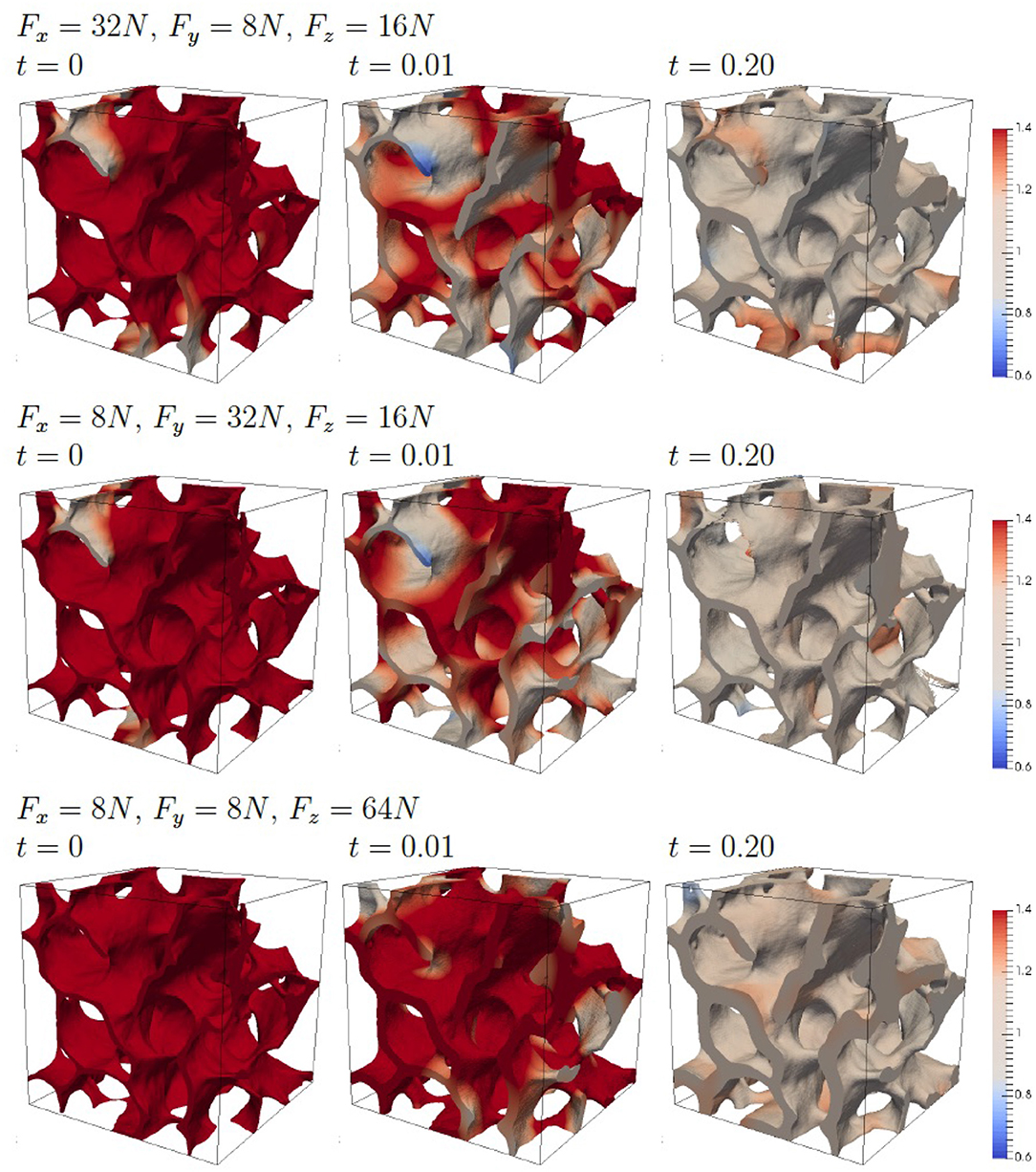
Figure 7. Evolution of the bone morphology with four-fold force in one direction. The color coding corresponds to the scaled concentration αc.

FIGURE 8

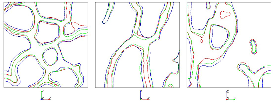
Figure 8. Comparison of the bone morphology along the xy-, xz-, and yz-plane (from left to right) at t = 0.20. Applied force is multiplied by a factor of 4 in direction x (red), y (green), or z (blue).

5. Discussion

We have introduced a continuous modeling approach for bone remodeling which has the potential to combine different scales in an efficient way. In the current form it combines elastic responds of the trabecular bone structure to an applied force, the concentration of signaling molecules within the bone and a mechanism how this concentration at the bone surface is used for local bone formation and resorption. In contrast to previous modeling approaches, using micro finite element analysis, the bone morphology is implicitly described by a time-dependent phase field function. This not only leads to a more accurate model, as the artificial voxel-roughness of the bone surface can be avoided, but also to a drastic reduction of system size and required computing time. The goal of this paper is to provide a minimal model for bone remodeling which demonstrates the advantages of the phase field description. We therefore not only introduce the model, but also quantitatively compare the results with established micro finite element approaches on simple geometries and consider the bone morphology within a segment of 2.84mm³ obtained from μCT data of a sheep vertebra with realistic parameters. Systematic studies with an enhanced force in one direction clearly demonstrate that the structures grow in the direction of the enhanced force and lead to strong local variations in thickness. These results clearly demonstrate the applicability of the phase field approach. However, quantitative validation would require in vivo μCT data of the trabecular bone segment and a calibration of the applied forces, which are currently not available. But already without such a validation the approach can be used to provide a deeper understanding of the mechanisms underlying bone remodeling. A possible extension considers the incorporation of osteoblast and osteoclast concentrations on the bone surface and their biochemical signaling, which will allow to compute the influence of various signaling molecules on the bone morphology. The ability to predict changes in bone morphology might eventually lead to a better prediction of individual fracture risk in osteoporotic patients or to improved implant materials. The introduced phase field description is ideally suited for this task, as it drastically reduces the computational cost, allows for extensions of additional effects and does only require standard numerical methods, which can be parallelized to deal with significantly larger systems.

Data Availability Statement

The raw data supporting the conclusions of this article will be made available by the authors, without undue reservation, to any qualified researcher.

Author Contributions

SA, AD, and AV designed the research. SA and AV developed the numerical model and wrote the manuscript. SA and RM performed numerical simulations. FS generated phase-fields from CT data. SA, RM, and AV analyzed the data.

Conflict of Interest

The authors declare that the research was conducted in the absence of any commercial or financial relationships that could be construed as a potential conflict of interest.

Acknowledgments

The authors acknowledge support by the German Research Foundation (DFG) through SFB/TRR 79 Materials for tissue regeneration within systemically altered bone (project M8, Z3, T1). We used computing resources provided by JSC within project HDR06 as well as resources provided by ZIH at TU Dresden. We acknowledge cooperation with M. Kampschulte, A. C. Langheinrich, T. El Khassawna, and C. Heiss. Publication of this article was funded by the Open Access Publication Fund of Hochschule für Technik und Wirtschaft Dresden University of Applied Sciences and the Deutsche Forschungsgemeinschaft (DFG, German Research Foundation)—432908064.

References

1. Huang C, Ogawa R. Mechanotransduction in bone repair and regeneration. FASEB J. (2010) 24:3625–32. doi: 10.1096/fj.10-157370

PubMed Abstract | CrossRef Full Text | Google Scholar

2. Jacobs CR, Temiyasathit S, Castillo AB. Osteocyte mechanobiology and pericellular mechanics. Annu Rev Biomed Eng. (2010) 12:369–400. doi: 10.1146/annurev-bioeng-070909-105302

PubMed Abstract | CrossRef Full Text | Google Scholar

3. Robling AG, Castillo AB, Turner CH. Biomechanical and biomolecular regulation of bone remodelling. Annu Rev Biomed Eng. (2006) 8:455–98. doi: 10.1146/annurev.bioeng.8.061505.095721

CrossRef Full Text | Google Scholar

4. Huiskes R, Ruimerman R, van Lenthe GH, Janssen JD. Effects of mechanical forces on maintenence and adaptation of form in trabecular bone. Nature. (2000) 405:704–6. doi: 10.1038/35015116

PubMed Abstract | CrossRef Full Text | Google Scholar

5. Dunlop JWC, Hartmann MA, Brechet YJ, Fratzl P, Weinkamer R. New suggestions for the mechanical control of bone remodeling. Calcif Tissue Int. (2009) 85:45–54. doi: 10.1007/s00223-009-9242-x

PubMed Abstract | CrossRef Full Text | Google Scholar

6. Fratzl P, Weinkamer R. Nature's hierarchical materials. Prog Mat Sci. (2007) 52:1263–334. doi: 10.1016/j.pmatsci.2007.06.001

CrossRef Full Text | Google Scholar

7. Ruimerman R, van Rietbergen B, Hilbers P, Huiskes R. The effect of trabecular bone loading variables on the surface signaling potential for bone remodeling and adaptation. Ann Biomed Eng. (2005) 33:71–8. doi: 10.1007/s10439-005-8964-9

CrossRef Full Text | Google Scholar

8. Tezuka K, Wada Y, Takahashi A, Kikuchi M. Computer-simulated bone architecture in a simple bone-remodeling model based on a reaction-diffusion system. J Bone Miner Metab. (2005) 23:1–7. doi: 10.1007/s00774-004-0533-z

PubMed Abstract | CrossRef Full Text | Google Scholar

9. Weinkamer R, Hartmann MA, Brechet Y, Fratzl P. Stochastic lattice model for bone remodeling and aging. Phys Rev Lett. (2004) 83:228102. doi: 10.1103/PhysRevLett.93.228102

CrossRef Full Text | Google Scholar

10. Adachi T, Tsubota K, Tomita Y, Hollister SJ. Trabecular surface remodeling simulation for cancellous bone using microstructural voxel finite element models. J Biomech Eng. (2001) 123:403–9. doi: 10.1115/1.1392315

PubMed Abstract | CrossRef Full Text | Google Scholar

11. McDonnell P, Harrison N, Liebscher MAK, Mc Hugh PE. Simulation of vertebral trabecular bone loss using voxel finite element analysis. J Biomech. (2009) 42:2789–96. doi: 10.1016/j.jbiomech.2009.07.038

CrossRef Full Text | Google Scholar

12. Ruimerman R, Hilbers P, van Rietbergen B, Huiskes R. A theoretical framework for strain-related trabecular bone maintenance and adaptation. J Biomech. (2005) 38:931–41. doi: 10.1016/j.jbiomech.2004.03.037

PubMed Abstract | CrossRef Full Text | Google Scholar

13. Schulte FA, Lambers FM, Webster DJ, Kuhn G, Müller R. In vivo validation of a computational bone adaptation model using open-loop control and time-lapsed micro-computed tomography. Bone. (2011) 49:1166–72. doi: 10.1016/j.bone.2011.08.018

PubMed Abstract | CrossRef Full Text | Google Scholar

14. Schulte FA, Zwahlen A, Lambers FM, Kuhn G, Ruffoni G, Betts D, et al. Strain-adaptive in silico modeling of bone adaptation - a computer simulation validated by in vivo micro-computed tomography data. Bone. (2013) 52:485–92. doi: 10.1016/j.bone.2012.09.008

PubMed Abstract | CrossRef Full Text | Google Scholar

15. Provatas N, Elder K (Editors). Phase-Field Methods in Materials Science and Engineering. Weinheim: Wiley-VCG (2010). doi: 10.1002/9783527631520

CrossRef Full Text | Google Scholar

16. Mauri R editor. Multiphase Microfluidics: The Diffuse Interface Model. Springer (2012). doi: 10.1007/978-3-7091-1227-4

CrossRef Full Text | Google Scholar

17. Li X, Lowengrub J, Rätz A, Voigt A. Solving PDE's in complex geometries: a diffuse domain approach. Commun Math Sci. (2009) 7:81–107. doi: 10.4310/CMS.2009.v7.n1.a4

CrossRef Full Text | Google Scholar

18. Aland S, Voigt A. Benchmark computations of diffuse interface models for two-dimensional bubble dynamics. Int J Numer Methods Fluids. (2012) 69:747–61. doi: 10.1002/fld.2611

CrossRef Full Text | Google Scholar

19. Aland S. Time integration for diffuse interface models for two-phase flow. J Comput Phys. (2014) 262:58–71. doi: 10.1016/j.jcp.2013.12.055

CrossRef Full Text | Google Scholar

20. Hensel R, Helbig R, Aland S, Braun HG, Voigt A, Neinhuis C, et al. Wetting resistance at its topographical limit: the benefit of mushroom and serif T structures. Langmuir. (2013) 29:1100–12. doi: 10.1021/la304179b

PubMed Abstract | CrossRef Full Text | Google Scholar

21. Aland S, Chen F. An efficient and energy stable scheme for a phase-field model for the moving contact line problem. Int J Numer Methods Fluids. (2016) 81:657–71. doi: 10.1002/fld.4200

CrossRef Full Text | Google Scholar

22. Aland S, Egerer S, Lowengrub J, Voigt A. Diffuse interface models of locally inextensible vesicles in a viscous fluid. J Comput Phys. (2014) 277:32–47. doi: 10.1016/j.jcp.2014.08.016

PubMed Abstract | CrossRef Full Text | Google Scholar

23. Aland S. Phase field models for two-phase flow with surfactants and biomembranes. In: Reusken A, Bothe D, editors. Transport Processes at Fluidic Interfaces. Cham: Birkhäuser (2017). p. 271–90. doi: 10.1007/978-3-319-56602-3_11

CrossRef Full Text | Google Scholar

24. Marth W, Aland S, Voigt A. Margination of white blood cells-a computational approach by a hydrodynamic phase field model. J Fluid Mech. (2016) 790:389–406. doi: 10.1017/jfm.2016.15

CrossRef Full Text | Google Scholar

25. Mokbel D, Abels H, Aland S. A phase-field model for fluid-structure-interaction. J Comput Phys. (2018) 372:823–40. doi: 10.1016/j.jcp.2018.06.063

CrossRef Full Text | Google Scholar

26. Aland S, Landsberg C, Müller R, Bobeth M, Langheinrich AC, Voigt A. Adaptive diffuse domain approach for calculating mechanically induced deformation of trabecular bone. Comput Meth Biomech Biomed Eng. (2014) 17:31–8. doi: 10.1080/10255842.2012.654606

PubMed Abstract | CrossRef Full Text | Google Scholar

27. Klein-Nulend J, Bakker AD, Bacabac RC, Vatsa A, Weinbaum S. Mechanosensation and transduction in osteocytes. Bone. (2013) 54:182–90. doi: 10.1016/j.bone.2012.10.013

PubMed Abstract | CrossRef Full Text | Google Scholar

28. Cowing SC, Moss-Salentijin L, Moss ML. Candidates for the mechanosensory system in bone. J Biomech Eng. (1991) 113:191–7. doi: 10.1115/1.2891234

CrossRef Full Text | Google Scholar

29. Komarova SV, Smith RJ, Dixon SJ, Sims SM, Wahl LM. Mathematical model predicts a critical role for osteoclast autocrine regulation in the control of bone remodeling. Bone. (2003) 33:206–15. doi: 10.1016/S8756-3282(03)00157-1

PubMed Abstract | CrossRef Full Text | Google Scholar

30. Lemaire V, Tobin FL, Greller LD, Cho CR, Suva LJ. Modeling the interactions between osteoblast and osteoclast activities in bone remodeling. J Theor Biol. (2004) 229:293–309. doi: 10.1016/j.jtbi.2004.03.023

PubMed Abstract | CrossRef Full Text | Google Scholar

31. Pivonke P, Zimak J, Smith DW, Gardinger BS, Dunstan CR, Sims NA, et al. Model structure and control of bone remodeling: a theoretical study. Bone. (2008) 43:249–63. doi: 10.1016/j.bone.2008.03.025

CrossRef Full Text | Google Scholar

32. Frost H. On our age-related bone loss: insights from a new paradigm. J Bone Miner Res. (1987) 12:1539–46. doi: 10.1359/jbmr.1997.12.10.1539

PubMed Abstract | CrossRef Full Text | Google Scholar

33. Oftadeh R, Perez-Viloria M, Villa-Camacho JC, Vaziri A, Nazarian A. Biomechanics and Mechanobiology of trabecular bone: a review. J Biomech Eng Trans ASME. (2015) 137:010802. doi: 10.1115/1.4029176

PubMed Abstract | CrossRef Full Text | Google Scholar

34. Keaveny TM, Guo XE, Wachtel EF, McMahon TA, Hayes WC. Trabecular bone exhibits fully linear elastic behavior and yields at low strains. J Biomech. (1994) 27:1127–36. doi: 10.1016/0021-9290(94)90053-1

PubMed Abstract | CrossRef Full Text | Google Scholar

35. Ladd AJC, Kinney JH, Haupt DL, Goldstein SA. Finite-element modelling of trabecular bone: Comparison with mechanical testing and determination of tissue modulus. J Orthep Res. (1998) 16:622–8. doi: 10.1002/jor.1100160516

CrossRef Full Text | Google Scholar

36. Levchuk A, Zwahlen A, Weigt C, Lambers FM, Badilatti SD, Schulte FA, et al. Large scale simulatiions of trabecular bone adaptation to loading and treatment. Clin Biomech. (2014) 29:355–62. doi: 10.1016/j.clinbiomech.2013.12.019

PubMed Abstract | CrossRef Full Text | Google Scholar

37. Podshivalov L, Fischer A, Bar-Yoseph PZ. 3D hierarchical geometric modeling and multiscale FE analysis as a base for individualized medical diagnosis of bone structure. Bone. (2011) 48:693–703. doi: 10.1016/j.bone.2010.12.022

PubMed Abstract | CrossRef Full Text | Google Scholar

38. Arbent P, van Lenthe GH, Mennel U, Müller R, Sala M. A scalable multi-level proconditioner for matrix-free μ-finite element analysis of human bone structures. Int J Num Meth Eng. (2008) 73:927–47. doi: 10.1002/nme.2101

CrossRef Full Text | Google Scholar

39. Landau LD, Lifshitz EM, Sykes JB, Reid WH, Dill EH. Theory of elasticity: vol. 7 of course of theoretical physics. Phys Today. (1960) 13:44. doi: 10.1063/1.3057037

CrossRef Full Text | Google Scholar

40. Folch R, Casademunt J, Hernandez-Machado A, Ramirez-Picina L. Phase-field model for Hele-Shaw flows with arbitrary viscosity contrast. I. Theoretical approach. Phys Rev E. (1999) 60:1725–33. doi: 10.1103/PhysRevE.60.1724

PubMed Abstract | CrossRef Full Text | Google Scholar

41. Voigt A, Witkowski T. A multi-mesh finite element method for Lagrange elements of arbitrary degree. J Comput Sci. (2012) 3:1612–28. doi: 10.1016/j.jocs.2012.06.004

CrossRef Full Text | Google Scholar

42. Ling S, Marth W, Praetorius S, Voigt A. An adaptive finite element multi-mesh approach for interacting deformable objects in flow. Comput Meth Appl Math. (2016) 16:475–84. doi: 10.1515/cmam-2016-0003

CrossRef Full Text | Google Scholar

43. Vey S, Voigt A. AMDiS - adaptive multidimensional simulations. Comput Vis Sci. (2007) 10:57–66. doi: 10.1007/s00791-006-0048-3

CrossRef Full Text | Google Scholar

44. Witkowski T, Ling S, Praetorius S, Voigt A. Software concepts and numerical algorithms for a scalable adaptive parallel finite element method. Adv Comput Math. (2015) 41:1145–77. doi: 10.1007/s10444-015-9405-4

CrossRef Full Text | Google Scholar

45. Mueller TL, Christen D, Sandercott S, Boyd SK, van Rietbergen B, Eckstein F, et al. Computational finite element bone mechanics accurately predicts mechanical competence in the human radius of an elderly population. Bone. (2011) 48:1232–8. doi: 10.1016/j.bone.2011.02.022

PubMed Abstract | CrossRef Full Text | Google Scholar

46. Müller R, Kampschulte M, Khassawna T, Schlewitz G, Hürter B, Böcker W, et al. Change of mechanical vertebrae properties due to progressive osteoporosis: combined biomechanical and finite-element analysis within a rat model. Med Bio Eng Comput. (2014) 52:405–14. doi: 10.1007/s11517-014-1140-3

PubMed Abstract | CrossRef Full Text | Google Scholar

47. Ehrlich PJ, Lanyon LE. Mechanical strain and bone cell function: a review. Osteoporosis Int. (2002) 13:688–700. doi: 10.1007/s001980200095

PubMed Abstract | CrossRef Full Text | Google Scholar