A Dynamical Systems Approach to Spectral Music: Modeling the Role of Roughness and Inharmonicity in Perception of Musical Tension

1. Introduction

Music gives rise to some of the strongest emotional experiences in our lives. Even though the first surviving theoretical treatments of the power of music to move the soul were written in the fifth century B.C. [1], the origin of this power still largely remains a mystery. However, both musicological and music-psychological evidence seems to converge on the theory that music arouses emotions by a sophisticated play of tension-resolution patterns [2]. For instance, many authors describe the musical language of Richard Wagner (1813–1883) as “the language of longing” [2]; it may not be merely a coincidence that Wagner's common practice was to introduce a dissonant chord, making the listener “long for” a more consonant chord to “resolve” the dissonance, and then keep the listener in tension by delaying the resolution or slap him right away with another dissonance [[2], p. 334–339].

Creating and resolving tension is an easy task for composers who follow the nineteenth century Western tradition (as, e.g., most “mainstream” composers of film music do); any standard textbook on harmony and voice leading provides them with plenty of recipes [e.g., [3]] tested by centuries of musical practice and decades of psychological research [e.g., [4] and references therein]. However, over the course of the twentieth century, many composers enriched their palette with sounds possessing neither definite pitch (precluding melody) nor perceivable voice structure (precluding harmony), thus venturing out into territories about which traditional theory has nothing to say but hic sunt leones [5]. Still, while tantalizing their audience with a sound palette ranging from pure tones to the most atrocious noises, they seek control over how their music is experienced by the listener as much as their more conservative colleagues do [6].

Devoid of any perceivable pitch structure, the ferocious sound materials contemporary art music is at times so fond of can only be conceived in terms of loudness and timbre. This forces any composer seeking a full control over these “beasts” to dive from the lofty heights of venerable musical abstractions like pitch, harmony, and tonality to the cold depths of spectral representations of sound. However, beauty emerges even from such depths; by careful manipulation of roughness and inharmonicity composers like Tristan Murail or Gérard Grisey “tense” their audience no less than Richard Wagner by his mastery of tonal harmony; indeed, the term “spectral music,” used when referring to the music style pioneered by the former two composers [7], does not tell the whole story.

As usual, music-psychological research somewhat lagged behind compositional practice; loud music has been shown to be perceived as more tense than soft music [8]; likewise, roughness (that is perception of rapid beating due to interference of close frequencies) seems to be positively correlated with tension [9, 10]. A recent study assessed the effect of specific timbre attributes on the perception of tension [11], confirming particularly the role of roughness, inharmonicity (deviation of the constituent frequencies from integer multiples of a fundamental tone) and spectral flatness. However, the functional forms and mechanisms through which such stimuli aspects combine to give rise to perceived tension are still unclear.

For standard Western musical intervals, roughness is a principal source of perceived dissonance in musical material, which thus gives rationale to mathematical models of musical dissonance [12]. In Stolzenburg [13], a mathematical model of dissonance has been proposed and shown to correlate highly with empirical psychophysical data. The core idea of the model can be illustrated on a simple example: Consider an interval of perfect fifth, the most consonant interval after the octave, which, in the standard Western tuning, corresponds to the distance of seven semitones. Hence, denoting f₁ and f₂ the fundamental frequencies of the tones spanning the interval, $[f_1,f_2]=[f_1,f_1{2}^{\frac{7}{12}}]$ ($2^{\frac{1}{12}}$ is the frequency ratio corresponding to a semitone distance in the standard Western tuning). First, approximate [f₁, f₂] with a pair of coprime natural numbers, Ω′ = [i, j], such that $\frac{i}{j}\approx \frac{f_1}{f_2}=2^{\frac{7}{12}}$, e.g., Ω′ = [2, 3]. Then, the dissonance of the interval will be 2, the minimum of Ω′. Likewise, for an interval of major sixth, considered less consonant than P5, with frequencies $[f_1,f_2]=[f_1,f_1{2}^{\frac{9}{12}}]$, we have Ω′ = [3, 5], the dissonance being 3 in this case. Finally, for a dissonant interval of minor seventh with frequencies $[f_1,f_2]=[f_1,f_1{2}^{\frac{9}{12}}]$, Ω′ = [4, 7] and the dissonance will be 4. In general, the dissonance of any vector of frequencies, f, approximated as ${\Omega }^{\prime }\in {\mathbb{Z}}_{\ge 1}^n$, is assumed to be proportional to the minimum element of Ω′. Note that the dissonance of an interval estimated this way does not change if we include harmonics (integer multiples) of the constituent frequencies. However, it does change if one uses a different rational approximation of the frequency ratio; incidentally, all standard Western intervals except for the octave are characterized by an irrational frequency ratio. In Stolzenburg [13], this inconvenience is dealt with by averaging over several alternative approximations.

The quantity above, called relative periodicity [see Definition 6 in [13], p. 17], is equivalent to obtaining the period of the fastest oscillation having the frequencies in question as its harmonics, in particular the period assessed in cycles of the lowest frequency in question. Interestingly, this oscillation has been experimentally observed to be represented in the auditory brainstem response to the intervals listed above [14], with the representation being particularly faithful for relatively more consonant intervals.

Motivated by the latter observation, we put forward a neurodynamical model of tension which is in line with the basic concepts of pitch perception of complex sounds and reproduces the results concerning the effect of roughness and inharmonicity reported in Farbood and Price [11] and, at the same time, provides a dynamical interpretation of relative periodicity [13]. In this regard we follow suit of existing studies which apply the dynamical systems theory to composition [15] and analysis [16, 17] of music.

2. Methods

Everyone interested in neurodynamical modeling faces the same basic dilemma: which model to use? For modeling perception of music, the most common choices are the leaky integrate-and-fire (LIF) model [18–21] and a canonical model for gradient-frequency networks of Wilson-Cowan-type neural oscillators [22–25]. Still, neuroimaging methods are far from giving us an assurance that among the myriad possible models one of these is the “correct” one. Hence, to improve our chances, instead of adhering to a particular model right from the beginning, we take a whole class of models as our point of departure in the hope that the class is wide enough to include a good approximation to the actual biological system. More precisely, we proceed by derivation of a normal form to which any of the class members can be transformed through a continuous near-identity change of variables and parameters and (possibly) a time scaling. Then, analysis of the entire class effectively reduces to analysis of the normal form [26].

The pioneering work of the latter approach in our field is Large et al. [22]; the model proposed therein can even be fit to auditory brainstem responses to musical intervals [24, 27]. Consequently, one could argue that we already have a neurodynamical model of tension at hand. However, to prove analytically that the latter is indeed a decent model of tension, we would first have to simplify the model substantially for the specific purpose, adopting thus a similar strategy as in previous applications of the model [23, 28, 29]. Moreover, the class of systems of which the latter is a canonical model [22, 27] is not the class of systems we are interested in, as shown below.

Our choice of model class is motivated by the observation that the auditory system is sensitive to the periodicity of the signal (see section 1). A possible explanation for the observation is that the system comprises an array of oscillatory “detectors” with external auditory signal input; these can be viewed (and indeed physically seem to be) ordered tonotopically with respect to their eigenfrequency. Within this framework, eliciting a sustained oscillation in one of the oscillators represents detection of the corresponding period in the input signal. Or, on a continuous scale, the more sustained an oscillation is, the more “‘confident” is the auditory system that the input signal exhibits the corresponding period. In order for a stimulus to elicit an oscillation in a model belonging to our class of choice, it needs to destabilize the (originally stable) quiescent state; if this shift in stability is relatively small or intermittent, the oscillation will have small or fluctuating amplitude.

To avoid introducing unnecessary complexity, we start building our model class of interest by considering the simplest possible model of an oscillator:

$\begin{array}{l}{\dot{x}}_1=-y_1\\ {\dot{y}}_1=x_1,\end{array}$

where x₁, y₁ ∈ ℝ and ẋ₁, ẏ₁ are time derivatives. In matrix form:

$\begin{array}{l}\left[\begin{array}{l}{\dot{x}}_1\\ {\dot{y}}_1\end{array}\right]=\left[\begin{array}{ll}0& -1\\ 1& \hfill 0\hfill \end{array}\right]\left[\begin{array}{l}{x}_1\\ y_1\end{array}\right].\end{array}$

Here, x₁ and y₁ could be interpreted as the amount of local inhibitory and excitatory synaptic activity, respectively, but the particular physiological interpretation of the variables is not important for our discussion. In line with the scenario outlined above, we want the oscillator to transit from a quiescent state (say, [x₁, y₁] = [0, 0]) to an oscillation when subject to an input having the oscillator's period (1 in this case). By definition, the spectrum of such an input consists of frequencies which are a subset of 1, 2, …, M. As we later aim to introduce the possibility of modeling the effect of inputs with frequencies deviating from perfect multiples of the base frequency, we allow already in the basic model for repeated frequency components of the input, yielding the input frequency vector [ω₁, ω₂, …, ω_n] = Ω = [1, 1, …, 1, 2, 2, …, 2, …, M, M, …, M], where M is the highest frequency contained in the input. Representing the i-th frequency component of the input with frequency ω_i as $[x_{i+1}(t),y_{i+1}(t)]\in {ℝ}^2$, we extend the oscillator with forcing by the input:

$\begin{array}{c}\left[\begin{array}{l}{\dot{x}}_1\\ {\dot{y}}_1\end{array}\right]=\left[\begin{array}{ll}0& -1\\ 1& \hfill 0\hfill \end{array}\right]\left[\begin{array}{l}{x}_1\\ y_1\end{array}\right]\\ +\left[\begin{array}{l}f(x_1,y_1,x_2(t),y_2(t),x_3(t),y_3(t),\dots ,x_{n+1}(t),y_{n+1}(t))\\ g(x_1,y_1,x_2(t),y_2(t),x_3(t),y_3(t),\dots ,x_{n+1}(t),y_{n+1}(t))\end{array}\right],\end{array}$

where f(·), g(·) are smooth real functions.

Two more steps are needed in order to make the model class amenable to derivation of a normal form. First, we need to rewrite this non-autonomous system as an autonomous one. This is straightforward, since [x_i+1(t), y_i+1(t)], being frequency components of a signal, are harmonic oscillations. Let x = [x₁, y₁, x₂, y₂, …, x_n+1, y_n+1]:

$\begin{array}{c}\hfill \dot{x}=\left[\begin{array}{ccccccccc}\hfill 0\hfill & \hfill -1\hfill & \hfill \hfill & \hfill \hfill & \hfill \hfill & \hfill \hfill & \hfill \hfill & \hfill \hfill & \hfill \hfill \\ \hfill 1\hfill & \hfill 0\hfill & \hfill \hfill & \hfill \hfill & \hfill \hfill & \hfill \hfill & \hfill \hfill & \hfill \hfill & \hfill \hfill \\ \hfill \hfill & \hfill \hfill & \hfill 0\hfill & \hfill -{\omega }_1\hfill & \hfill \hfill & \hfill \hfill & \hfill \hfill & \hfill \hfill & \hfill \hfill \\ \hfill \hfill & \hfill \hfill & \hfill {\omega }_1\hfill & \hfill 0\hfill & \hfill \hfill & \hfill \hfill & \hfill \hfill & \hfill \hfill & \hfill \hfill \\ \hfill \hfill & \hfill \hfill & \hfill \hfill & \hfill \hfill & \hfill 0\hfill & \hfill -{\omega }_2\hfill & \hfill \hfill & \hfill \hfill & \hfill \hfill \\ \hfill \hfill & \hfill \hfill & \hfill \hfill & \hfill \hfill & \hfill {\omega }_2\hfill & \hfill 0\hfill & \hfill \hfill & \hfill \hfill & \hfill \hfill \\ \hfill \hfill & \hfill \hfill & \hfill \hfill & \hfill \hfill & \hfill \hfill & \hfill \hfill & \hfill \ddots \hfill & \hfill \hfill & \hfill \hfill \\ \hfill \hfill & \hfill \hfill & \hfill \hfill & \hfill \hfill & \hfill \hfill & \hfill \hfill & \hfill \hfill & \hfill 0\hfill & \hfill -{\omega }_n\hfill \\ \hfill \hfill & \hfill \hfill & \hfill \hfill & \hfill \hfill & \hfill \hfill & \hfill \hfill & \hfill \hfill & \hfill {\omega }_n\hfill & \hfill 0\hfill \end{array}\right]x+\left[\begin{array}{c}\hfill f\left(x\right)\hfill \\ \hfill g\left(x\right)\hfill \\ \hfill 0\hfill \\ \hfill 0\hfill \\ \hfill 0\hfill \\ \hfill 0\hfill \\ \hfill ⋮\hfill \\ \hfill 0\hfill \\ \hfill 0\hfill \end{array}\right].\hfill \end{array}$

Second, we expand the f(·) and g(·) functions around the origin:

$\begin{array}{c}\hfill \dot{x}=\left[\begin{array}{ccccccccc}\hfill 0\hfill & \hfill -1\hfill & \hfill \hfill & \hfill \hfill & \hfill \hfill & \hfill \hfill & \hfill \hfill & \hfill \hfill & \hfill \hfill \\ \hfill 1\hfill & \hfill 0\hfill & \hfill \hfill & \hfill \hfill & \hfill \hfill & \hfill \hfill & \hfill \hfill & \hfill \hfill & \hfill \hfill \\ \hfill \hfill & \hfill \hfill & \hfill 0\hfill & \hfill -{\omega }_1\hfill & \hfill \hfill & \hfill \hfill & \hfill \hfill & \hfill \hfill & \hfill \hfill \\ \hfill \hfill & \hfill \hfill & \hfill {\omega }_1\hfill & \hfill 0\hfill & \hfill \hfill & \hfill \hfill & \hfill \hfill & \hfill \hfill & \hfill \hfill \\ \hfill \hfill & \hfill \hfill & \hfill \hfill & \hfill \hfill & \hfill 0\hfill & \hfill -{\omega }_2\hfill & \hfill \hfill & \hfill \hfill & \hfill \hfill \\ \hfill \hfill & \hfill \hfill & \hfill \hfill & \hfill \hfill & \hfill {\omega }_2\hfill & \hfill 0\hfill & \hfill \hfill & \hfill \hfill & \hfill \hfill \\ \hfill \hfill & \hfill \hfill & \hfill \hfill & \hfill \hfill & \hfill \hfill & \hfill \hfill & \hfill \ddots \hfill & \hfill \hfill & \hfill \hfill \\ \hfill \hfill & \hfill \hfill & \hfill \hfill & \hfill \hfill & \hfill \hfill & \hfill \hfill & \hfill \hfill & \hfill 0\hfill & \hfill -{\omega }_n\hfill \\ \hfill \hfill & \hfill \hfill & \hfill \hfill & \hfill \hfill & \hfill \hfill & \hfill \hfill & \hfill \hfill & \hfill {\omega }_n\hfill & \hfill 0\hfill \end{array}\right]x+\left[\begin{array}{c}\hfill f_2\left(x\right)\hfill \\ \hfill g_2\left(x\right)\hfill \\ \hfill 0\hfill \\ \hfill 0\hfill \\ \hfill 0\hfill \\ \hfill 0\hfill \\ \hfill ⋮\hfill \\ \hfill 0\hfill \\ \hfill 0\hfill \end{array}\right]\hfill \\ \hfill +\left[\begin{array}{c}\hfill f_3\left(x\right)\hfill \\ \hfill g_3\left(x\right)\hfill \\ \hfill 0\hfill \\ \hfill 0\hfill \\ \hfill 0\hfill \\ \hfill 0\hfill \\ \hfill ⋮\hfill \\ \hfill 0\hfill \\ \hfill 0\hfill \end{array}\right]+\left[\begin{array}{c}\hfill {O}\left(x^4\right)\hfill \\ \hfill {O}\left(x^4\right)\hfill \\ \hfill 0\hfill \\ \hfill 0\hfill \\ \hfill 0\hfill \\ \hfill 0\hfill \\ \hfill ⋮\hfill \\ \hfill 0\hfill \\ \hfill 0\hfill \end{array}\right],\hfill & (1)\end{array}$

where f_d(x), g_d(x) are homogeneous polynomials of degree d and ${O}(x^4)$ is a polynomial of degree 4 or more.

Before delving into the actual derivation, a few remarks are in place. First, the idea of modeling the auditory system as a tonotopically arranged array (or rather a series of arrays) of oscillators is in fact not new [23, 24, 27]. Further, since the lowest frequency of signal with harmonic spectrum corresponds to its perceived pitch, Equation (1) is, by design, a pitch detector. Then, instantiating Equation (1) with a range of eigenfrequencies can be thought of as matching a template to the signal; consequently, our model can be considered a neurodynamical implementation of template matching postulated as a possible mechanism underlying pitch perception [30].

As the first step of the derivation, we diagonalize the linear part of Equation (1) using the following two matrices:

$\begin{array}{c}\hfill T=\frac{1}{2}\left[\begin{array}{ccccccccc}\hfill 1\hfill & \hfill 1\hfill & \hfill \hfill & \hfill \hfill & \hfill \hfill & \hfill \hfill & \hfill \hfill & \hfill \hfill & \hfill \hfill \\ \hfill -\iota \hfill & \hfill \iota \hfill & \hfill \hfill & \hfill \hfill & \hfill \hfill & \hfill \hfill & \hfill \hfill & \hfill \hfill & \hfill \hfill \\ \hfill \hfill & \hfill \hfill & \hfill 1\hfill & \hfill 1\hfill & \hfill \hfill & \hfill \hfill & \hfill \hfill & \hfill \hfill & \hfill \hfill \\ \hfill \hfill & \hfill \hfill & \hfill -\iota \hfill & \hfill \iota \hfill & \hfill \hfill & \hfill \hfill & \hfill \hfill & \hfill \hfill & \hfill \hfill \\ \hfill \hfill & \hfill \hfill & \hfill \hfill & \hfill \hfill & \hfill 1\hfill & \hfill 1\hfill & \hfill \hfill & \hfill \hfill & \hfill \hfill \\ \hfill \hfill & \hfill \hfill & \hfill \hfill & \hfill \hfill & \hfill -\iota \hfill & \hfill \iota \hfill & \hfill \hfill & \hfill \hfill & \hfill \hfill \\ \hfill \hfill & \hfill \hfill & \hfill \hfill & \hfill \hfill & \hfill \hfill & \hfill \hfill & \hfill \ddots \hfill & \hfill \hfill & \hfill \hfill \\ \hfill \hfill & \hfill \hfill & \hfill \hfill & \hfill \hfill & \hfill \hfill & \hfill \hfill & \hfill \hfill & \hfill 1\hfill & \hfill 1\hfill \\ \hfill \hfill & \hfill \hfill & \hfill \hfill & \hfill \hfill & \hfill \hfill & \hfill \hfill & \hfill \hfill & \hfill \iota \hfill & \hfill -\iota \hfill \end{array}\right],\hfill \\ T^{-1}=\left[\begin{array}{ccccccccc}\hfill 1\hfill & \hfill \iota \hfill & \hfill \hfill & \hfill \hfill & \hfill \hfill & \hfill \hfill & \hfill \hfill & \hfill \hfill & \hfill \hfill \\ \hfill 1\hfill & \hfill -\iota \hfill & \hfill \hfill & \hfill \hfill & \hfill \hfill & \hfill \hfill & \hfill \hfill & \hfill \hfill & \hfill \hfill \\ \hfill \hfill & \hfill \hfill & \hfill 1\hfill & \hfill \iota \hfill & \hfill \hfill & \hfill \hfill & \hfill \hfill & \hfill \hfill & \hfill \hfill \\ \hfill \hfill & \hfill \hfill & \hfill 1\hfill & \hfill -\iota \hfill & \hfill \hfill & \hfill \hfill & \hfill \hfill & \hfill \hfill & \hfill \hfill \\ \hfill \hfill & \hfill \hfill & \hfill \hfill & \hfill \hfill & \hfill 1\hfill & \hfill \iota \hfill & \hfill \hfill & \hfill \hfill & \hfill \hfill \\ \hfill \hfill & \hfill \hfill & \hfill \hfill & \hfill \hfill & \hfill 1\hfill & \hfill -\iota \hfill & \hfill \hfill & \hfill \hfill & \hfill \hfill \\ \hfill \hfill & \hfill \hfill & \hfill \hfill & \hfill \hfill & \hfill \hfill & \hfill \hfill & \hfill \ddots \hfill & \hfill \hfill & \hfill \hfill \\ \hfill \hfill & \hfill \hfill & \hfill \hfill & \hfill \hfill & \hfill \hfill & \hfill \hfill & \hfill \hfill & \hfill 1\hfill & \hfill \iota \hfill \\ \hfill \hfill & \hfill \hfill & \hfill \hfill & \hfill \hfill & \hfill \hfill & \hfill \hfill & \hfill \hfill & \hfill 1\hfill & \hfill -\iota \hfill \end{array}\right],\hfill \end{array}$

where ι is the imaginary unit. Denoting the linear part of Equation (1) as A, the diagonalized matrix reads:

$\begin{array}{ll}{T}^{-1}AT=\left[\begin{array}{ccccccccc}\hfill \iota \hfill & \hfill \hfill & \hfill \hfill & \hfill \hfill & \hfill \hfill & \hfill \hfill & \hfill \hfill & \hfill \hfill & \hfill \hfill \\ \hfill \hfill & \hfill -\iota \hfill & \hfill \hfill & \hfill \hfill & \hfill \hfill & \hfill \hfill & \hfill \hfill & \hfill \hfill & \hfill \hfill \\ \hfill \hfill & \hfill \hfill & \hfill \iota {\omega }_1\hfill & \hfill \hfill & \hfill \hfill & \hfill \hfill & \hfill \hfill & \hfill \hfill & \hfill \hfill \\ \hfill \hfill & \hfill \hfill & \hfill \hfill & \hfill -\iota {\omega }_1\hfill & \hfill \hfill & \hfill \hfill & \hfill \hfill & \hfill \hfill & \hfill \hfill \\ \hfill \hfill & \hfill \hfill & \hfill \hfill & \hfill \hfill & \hfill \iota {\omega }_2\hfill & \hfill \hfill & \hfill \hfill & \hfill \hfill & \hfill \hfill \\ \hfill \hfill & \hfill \hfill & \hfill \hfill & \hfill \hfill & \hfill \hfill & \hfill -\iota {\omega }_2\hfill & \hfill \hfill & \hfill \hfill & \hfill \hfill \\ \hfill \hfill & \hfill \hfill & \hfill \hfill & \hfill \hfill & \hfill \hfill & \hfill \hfill & \hfill \ddots \hfill & \hfill \hfill & \hfill \hfill \\ \hfill \hfill & \hfill \hfill & \hfill \hfill & \hfill \hfill & \hfill \hfill & \hfill \hfill & \hfill \hfill & \hfill \iota {\omega }_n\hfill & \hfill \hfill \\ \hfill \hfill & \hfill \hfill & \hfill \hfill & \hfill \hfill & \hfill \hfill & \hfill \hfill & \hfill \hfill & \hfill \hfill & \hfill -\iota {\omega }_n\hfill \end{array}\right].& (2)\end{array}$

The diagonalization defines a change of variables:

$\begin{array}{c}\hfill \left[\begin{array}{c}\hfill z_1\hfill \\ \hfill w_1\hfill \\ \hfill z_2\hfill \\ \hfill w_2\hfill \\ \hfill z_3\hfill \\ \hfill w_3\hfill \\ \hfill ⋮\hfill \\ \hfill z_{n+1}\hfill \\ \hfill w_{n+1}\hfill \end{array}\right]=\varsigma =T^{-1}x=\left[\begin{array}{ccccccccc}\hfill 1\hfill & \hfill \iota \hfill & \hfill \hfill & \hfill \hfill & \hfill \hfill & \hfill \hfill & \hfill \hfill & \hfill \hfill & \hfill \hfill \\ \hfill 1\hfill & \hfill -\iota \hfill & \hfill \hfill & \hfill \hfill & \hfill \hfill & \hfill \hfill & \hfill \hfill & \hfill \hfill & \hfill \hfill \\ \hfill \hfill & \hfill \hfill & \hfill 1\hfill & \hfill \iota \hfill & \hfill \hfill & \hfill \hfill & \hfill \hfill & \hfill \hfill & \hfill \hfill \\ \hfill \hfill & \hfill \hfill & \hfill 1\hfill & \hfill -\iota \hfill & \hfill \hfill & \hfill \hfill & \hfill \hfill & \hfill \hfill & \hfill \hfill \\ \hfill \hfill & \hfill \hfill & \hfill \hfill & \hfill \hfill & \hfill 1\hfill & \hfill \iota \hfill & \hfill \hfill & \hfill \hfill & \hfill \hfill \\ \hfill \hfill & \hfill \hfill & \hfill \hfill & \hfill \hfill & \hfill 1\hfill & \hfill -\iota \hfill & \hfill \hfill & \hfill \hfill & \hfill \hfill \\ \hfill \hfill & \hfill \hfill & \hfill \hfill & \hfill \hfill & \hfill \hfill & \hfill \hfill & \hfill \ddots \hfill & \hfill \hfill & \hfill \hfill \\ \hfill \hfill & \hfill \hfill & \hfill \hfill & \hfill \hfill & \hfill \hfill & \hfill \hfill & \hfill \hfill & \hfill 1\hfill & \hfill \iota \hfill \\ \hfill \hfill & \hfill \hfill & \hfill \hfill & \hfill \hfill & \hfill \hfill & \hfill \hfill & \hfill \hfill & \hfill 1\hfill & \hfill -\iota \hfill \end{array}\right]\left[\begin{array}{c}\hfill x_1\hfill \\ \hfill y_1\hfill \\ \hfill x_2\hfill \\ \hfill y_2\hfill \\ \hfill x_3\hfill \\ \hfill y_3\hfill \\ \hfill ⋮\hfill \\ \hfill x_{n+1}\hfill \\ \hfill y_{n+1}\hfill \end{array}\right]\hfill \\ \hfill =\left[\begin{array}{c}\hfill x_1+\iota y_1\hfill \\ \hfill x_1-\iota y_1\hfill \\ \hfill x_2+\iota y_2\hfill \\ \hfill x_2-\iota y_2\hfill \\ \hfill x_3+\iota y_3\hfill \\ \hfill x_3-\iota y_3\hfill \\ \hfill ⋮\hfill \\ \hfill x_{n+1}+\iota y_{n+1}\hfill \\ \hfill x_{n+1}-\iota y_{n+1}\hfill \end{array}\right].\hfill \end{array}$

After this change, Equation (1) reads:

$\begin{array}{l}\dot{z_k}=\dot{x_k}+\iota \dot{y_k}=\\ =\{\begin{array}{cc}-y_k+\iota x_k+f(x)={\iota }^2{y}_k+\iota x_k+f(x)\hfill & k=1\hfill \\ =\iota z_k+f_{zeta}(\zeta ),\hfill \\ \iota {\omega }_{k-1}{z}_k,\hfill & 1<k\le n\hfill \end{array}& (3)\end{array}$

$\begin{array}{l}\dot{w_k}=\dot{x_k}-\iota \dot{y_k}=\\ =\{\begin{array}{cc}-y_k-\iota x_k+g(x)={\iota }^2{y}_k-\iota x_k+g(x)\hfill & k=1\hfill \\ =-\iota w_k+g_{\zeta }(\zeta ),\hfill \\ -\iota {\omega }_{k-1}{w}_k,\hfill & 1<k\le n,\end{array}& (4)\end{array}$

with $g_{\zeta }(\zeta )=\overline{f_{\zeta }}(\zeta )$, where and $\overline{·}$ is complex conjugate. From here, with a slight abuse of notation, we drop for simplicity the subscript of g_ζ(ζ) which is a function in the complex vector space corresponding to g(x) from section 2, that is obtained through the change of variables applied, i.e., $g_{\zeta }(\zeta )=g_{\zeta }(T^{-1}x)=g(x)$; likewise for f(ζ). Our subject of study will be the normal form of the system comprising Equations (3) and (4).

When in normal form, f(ζ) in Equation (3) will only contain monomials of the form

$\begin{array}{ll}{c}_{rspq}{z}^{\left[r,p\right]}{w}^{\left[s,q\right]}=c_{rspq}{z}_1^r{z}_2^{p_1}{z}_3^{p_2}\cdots z_{n+1}^{p_n}{w}_1^s{w}_2^{q_1}{w}_3^{q_2}\cdots w_{n+1}^{q_n},& (5)\end{array}$

where p = [p₁, p₂, …, p_n], q = [q₁, q₂, …, q_n], and [r, s, p, q] is a nonnegative integer solution to the equation

$\begin{array}{ll}r-s+p\Omega -q\Omega =1.& (6)\end{array}$

Analogously, the exponents in g(ζ) solve

$\begin{array}{ll}r-s+p\Omega -q\Omega =-1& (7)\end{array}$

(see Equation 2). Since f(ζ) and g(ζ) contain neither constant nor linear terms (see section 2),

$\begin{array}{l}r+s+\left|p\right|+\left|q\right|=r+s+(p_1+p_2+\cdots +p_n)+(q_1+q_2+\cdots +q_n)\ge 2.\end{array}$

For conciseness, from now on, whenever v = [r, s, p, q] satisfies the above inequality, we write v ∈ S when it solves Equation (6) and $v\in \tilde{S}$ when it solves Equation (7). Note that [r, s, p, q] ∈ S iff $[s,r,q,p]\in \tilde{S}$. Consequently, in the normal form,

$\begin{array}{l}g(\zeta )={\displaystyle \sum _{\left[r,s,p,q\right]\in \tilde{S}}}{c}_{rspq}{z}^{\left[r,p\right]}{w}^{\left[s,q\right]}={\displaystyle \sum _{\left[r,s,p,q\right]\in S}}{c}_{srqp}{z}^{\left[s,q\right]}{w}^{\left[r,p\right]}=\\ \overline{f(\zeta )}={\displaystyle \sum _{\left[r,s,p,q\right]\in S}}\overline{c_{rspq}}{\overline{z}}^{\left[r,p\right]}{\overline{w}}^{\left[s,q\right]}={\displaystyle \sum _{\left[r,s,p,q\right]\in S}}\overline{c_{rspq}}{w}^{\left[r,p\right]}{z}^{\left[s,q\right]}\end{array}$

and, by equality of polynomials,

$\begin{array}{l}{c}_{srqp}=\overline{c_{rspq}}\end{array}$

for all [r, s, p, q] ∈ S.

To broaden the class of systems covered by our normal form, we unfold Equation (3) using small parameters α ∈ ℝ and β ∈ ℝⁿ:

$\begin{array}{l}\dot{z_k}=\{\begin{array}{cc}(\alpha +\iota )z_k+f(\zeta ),\hfill & k=1\hfill \\ (\iota +\iota {\beta }_{k-1}){\omega }_{k-1}{z}_k,\hfill & k\ge 2\hfill \end{array}\hfill \\ \dot{w_k}=\{\begin{array}{cc}(\alpha -\iota )w_k+g(\zeta ),\hfill & k=1\hfill \\ (-\iota -\iota {\beta }_{k-1}){\omega }_{k-1}{w}_k,\hfill & k\ge 2\hfill \end{array}.\hfill \end{array}$

This way, in addition to the models with Taylor expansion around the origin of the form (Equation 1), our class now includes models whose Taylor expansion around the origin has the form

$\begin{array}{ll}\begin{array}{c}\hfill \dot{x}=\left[\begin{array}{ccccccccc}\hfill \alpha \hfill & \hfill -1\hfill & \hfill \hfill & \hfill \hfill & \hfill \hfill & \hfill \hfill & \hfill \hfill & \hfill \hfill & \hfill \hfill \\ \hfill 1\hfill & \hfill \alpha \hfill & \hfill \hfill & \hfill \hfill & \hfill \hfill & \hfill \hfill & \hfill \hfill & \hfill \hfill & \hfill \hfill \\ \hfill \hfill & \hfill \hfill & \hfill \iota {\omega }_1{\beta }_1\hfill & \hfill -{\omega }_1\hfill & \hfill \hfill & \hfill \hfill & \hfill \hfill & \hfill \hfill & \hfill \hfill \\ \hfill \hfill & \hfill \hfill & \hfill {\omega }_1\hfill & \hfill -\iota {\omega }_1{\beta }_1\hfill & \hfill \hfill & \hfill \hfill & \hfill \hfill & \hfill \hfill & \hfill \hfill \\ \hfill \hfill & \hfill \hfill & \hfill \hfill & \hfill \hfill & \hfill \iota {\omega }_2{\beta }_2\hfill & \hfill -{\omega }_2\hfill & \hfill \hfill & \hfill \hfill & \hfill \hfill \\ \hfill \hfill & \hfill \hfill & \hfill \hfill & \hfill \hfill & \hfill {\omega }_2\hfill & \hfill -\iota {\omega }_2{\beta }_2\hfill & \hfill \hfill & \hfill \hfill & \hfill \hfill \\ \hfill \hfill & \hfill \hfill & \hfill \hfill & \hfill \hfill & \hfill \hfill & \hfill \hfill & \hfill \ddots \hfill & \hfill \hfill & \hfill \hfill \\ \hfill \hfill & \hfill \hfill & \hfill \hfill & \hfill \hfill & \hfill \hfill & \hfill \hfill & \hfill \hfill & \hfill \iota {\omega }_n{\beta }_n\hfill & \hfill -{\omega }_n\hfill \\ \hfill \hfill & \hfill \hfill & \hfill \hfill & \hfill \hfill & \hfill \hfill & \hfill \hfill & \hfill \hfill & \hfill {\omega }_n\hfill & \hfill -\iota {\omega }_n{\beta }_n\hfill \end{array}\right]x\hfill \\ \hfill +\left[\begin{array}{c}\hfill f_2\left(x\right)\hfill \\ \hfill g_2\left(x\right)\hfill \\ \hfill 0\hfill \\ \hfill 0\hfill \\ \hfill 0\hfill \\ \hfill 0\hfill \\ \hfill ⋮\hfill \\ \hfill 0\hfill \\ \hfill 0\hfill \end{array}\right]+\left[\begin{array}{c}\hfill f_3\left(x\right)\hfill \\ \hfill g_3\left(x\right)\hfill \\ \hfill 0\hfill \\ \hfill 0\hfill \\ \hfill 0\hfill \\ \hfill 0\hfill \\ \hfill ⋮\hfill \\ \hfill 0\hfill \\ \hfill 0\hfill \end{array}\right]+\left[\begin{array}{c}\hfill {O}\left(x^4\right)\hfill \\ \hfill {O}\left(x^4\right)\hfill \\ \hfill 0\hfill \\ \hfill 0\hfill \\ \hfill 0\hfill \\ \hfill 0\hfill \\ \hfill ⋮\hfill \\ \hfill 0\hfill \\ \hfill 0\hfill \end{array}\right].\hfill \end{array}& (8)\end{array}$

The corresponding normal form then reads

$\begin{array}{l}\dot{z_1}=(\alpha +\iota )z_1+{\displaystyle \sum _{\left[r,s,p,q\right]\in S}}{c}_{rspq}{z}^{\left[r,p\right]}{w}^{\left[s,q\right]}\\ \dot{w_1}=(\alpha -\iota )w_1+{\displaystyle \sum _{\left[r,s,p,q\right]\in S}}\overline{c_{rspq}}{z}^{\left[s,q\right]}{w}^{\left[r,p\right]}\\ \dot{z_2}=\iota (1+{\beta }_1){\omega }_1{z}_2\\ \dot{w_2}=-\iota (1+{\beta }_1){\omega }_1{w}_2\\ \dot{z_3}=\iota (1+{\beta }_2){\omega }_2{z}_3\\ \dot{w_3}=-\iota (1+{\beta }_2){\omega }_2{w}_3\\ ⋮\\ \dot{z_{n+1}}=\iota (1+{\beta }_n){\omega }_n{z}_{n+1}\\ \dot{w_{n+1}}=-\iota (1+{\beta }_n){\omega }_n{w}_{n+1}.& (9)\end{array}$

Intuitively, the α parameter makes it possible to change the stability of the origin (see section 2.1) whereas the β_k parameters allow the model to resonate when the inputs are not exactly its harmonics. In fact, it might happen that two different inputs approximate the same harmonic. That is, their frequencies equal (1 + β_i)ω_i and (1 + β_j)ω_j, respectively, with ω_i = ω_j. This is the reason why we allowed for duplicate frequencies in the input frequency vector Ω (see the beginning of section 2).

It might appear that Equation (9) only models period detection in a full harmonic spectrum (up to the n-th harmonic). However, it can be easily adapted to a more general stimulus with frequencies H^harm ⊂ Ω by removing the dependence on those z_j and w_j for which ${\Omega }_j\notin H^{\text{harm}}$ from the equation for ż₁ and ẇ₁ (assuming the dimension of the system is large enough to accommodate any stimulus of practical interest). Since the right-hand sides of the equations are polynomials, it suffices to zero-out the coefficients of those terms containing nonzero powers of the offending z_j or w_j. This will turn out to be useful when extending the model to an array by making scaled copies of Equation (9); while changing the eigenfrequency by scaling the left-hand side, we can zero-out coefficients as needed to reflect the changing relation between the eigenfrequency and the inputs.

It might be interesting to compare Equation (9) to [[22], Equation 15] reproduced below in a form that facilitates the comparison [see also [27], Equation A.1], which is also a normal form for an oscillator coupled to a set of sinusoidal inputs:

$\begin{array}{ll}{ż}_1=(\alpha +\iota )z_1+{\displaystyle \sum _{\left[r,s,p,q\right]}}{c}_{rspq}{z}^{\left[r,p\right]}{w}^{\left[s,q\right]},& (10)\end{array}$

where

$\begin{array}{ll}{c}_{rspq}=\{\begin{array}{cc}{d}_{rspq}\hfill & p=q=0\hfill \\ {\sqrt{ϵ}}^{s+\left|p\right|+\left|q\right|-1}\hfill & \text{otherwise.}\hfill \end{array}\hfill & (11)\end{array}$

In Equation (10), the sum runs over all such vectors [r, s, p, q] for which either r = s + 1, s ∈ ℤ_>0, p = q = 0, or r = 0, s ∈ ℤ_≥0, $p,q\in {\mathbb{Z}}_{\ge 0}^n$, r + s + |p| + |q| > 0. In contrast, the sum in Equation (9) only runs over the nonnegative solutions to Equation (6), whose coefficients are determined by input frequencies. Hence, whereas Equation (10) applies to inputs of arbitrary frequencies, Equation (9) requires that the frequencies are close to the harmonics of the oscillator's eigenfrequency. On the other hand, in contrast to Equation (9), Equation (10) presupposes a particular form of the coefficients (see Equation 11). Consequently, Equation (9) covers neither a subset, nor a superset of the models covered by Equation (10).

2.1. Model Analysis

In this subsection, we analyse the normal form (Equation 9) derived in section 2. More precisely, we study the stability of the origin (z₁ = w₁ = 0). The choice of the origin as the focus of this section is motivated by our previous (arbitrary) choice of the origin as a “quiescent state” of the oscillator (see the beginning of section 2). The reason why we treat its stability in such a detail here is that it determines whether, e.g., the oscillator stays quiet (its period was not detected in the input signal) or oscillates (its period was detected in the signal)—see the beginning of section 2.

As the first step of the analysis, note that all solutions to Equation (9) are of the form

$\begin{array}{l}\left[z_1,z_2,z_3,\dots ,z_{n+1}\right]\\ =\left[z_1(t),{\rho }_1{e}^{\iota (1+{\beta }_1){\omega }_{1}t},{\rho }_2{e}^{\iota ({\phi }_2+(1+{\beta }_2){\omega }_{2}t)},\dots ,{\rho }_n{e}^{\iota ({\phi }_n+(1+{\beta }_n){\omega }_{n}t)}\right]\\ \left[w_1,w_2,w_3,\dots ,w_{n+1}\right]\\ =\left[w_1,{\rho }_1{e}^{-\iota (1+{\beta }_1){\omega }_{1}t},{\rho }_2{e}^{-\iota ({\phi }_2+(1+{\beta }_2){\omega }_{2}t)},\dots ,{\rho }_n{e}^{-\iota ({\phi }_n+(1+{\beta }_n){\omega }_{n}t)}\right].& (12)\end{array}$

Consequently, using the simplified notation Ω = [1, 1, …, 1, 2, 2, …, 2, …, N, N, …, N] and β = [β₁, β₂, …, β_n] as above, and introducing ρ = [ρ₁, ρ₂, …, ρ_n], φ = [0, φ₂, …, φ_n], and Ω_β = Ω ◦ β = [ω₁ β ₁, …, ω_n β _n], we can drop equations for ż₂, ż₃, …, ż_n+1 and ẇ₂, ẇ₃, …, ẇ_n+1 from Equation (9) and write

$\begin{array}{l}\dot{z_1}=(\alpha +\iota )z_1\\ +{\displaystyle \sum _{\left[r,s,p,q\right]\in S}}{c}_{rspq}{z}_1^r{w}_1^s{\rho }^{p+q}{e}^{\iota (p\phi -q\phi )}{e}^{\iota (p(\Omega +{\Omega }_{\beta })-q(\Omega +{\Omega }_{\beta }))t}\\ \dot{w_1}=(\alpha -\iota )w_1\\ +{\displaystyle \sum _{\left[r,s,p,q\right]\in S}}\overline{c_{rspq}}{z}_1^s{w}_1^r{\rho }^{p+q}{e}^{\iota (q\phi -p\phi )}{e}^{\iota (q(\Omega +{\Omega }_{\beta })-p(\Omega +{\Omega }_{\beta }))t}.& (13)\end{array}$

Introducing new coordinates relative to a rotating frame of reference e^ιt,

$\begin{array}{l}u=z_1{e}^{-\iota t}\\ v=w_1{e}^{\iota t},& (14)\end{array}$

and new parameters,

$\begin{array}{ll}{\Delta }_{pq}=p{\Omega }_{\beta }-q{\Omega }_{\beta },& (15)\end{array}$

Equation (13) reduces to:

$\begin{array}{l}\dot{u}=\dot{z_1}{e}^{-\iota t}-\iota z_1{e}^{-\iota t}=e^{-\iota t}(\dot{z_1}-\iota z_1)\\ =\alpha u+{\displaystyle \sum _{\left[r,s,p,q\right]\in S}}{c}_{rspq}{u}^r{v}^s{\rho }^{p+q}{e}^{\iota (p\phi -q\phi )}{e}^{\iota {\Delta }_{pq}t}& (16)\end{array}$

$\begin{array}{l}\dot{v}=\dot{w_1}{e}^{\iota t}+\iota w_1{e}^{\iota t}=e^{\iota t}(\dot{w_1}+\iota w_1)\\ =\alpha v+{\displaystyle \sum _{\left[r,s,p,q\right]\in S}}\overline{c_{rspq}}{u}^s{v}^r{\rho }^{p+q}{e}^{\iota (q\phi -p\phi )}{e}^{-\iota {\Delta }_{pq}t}.& (17)\end{array}$

As we will see in section 3, under a rather generic restriction on Equations (16) and (17), the stability of u = v = 0 crucially depends on the relative periodicity and the inharmonicity of the input, as formalized in previous studies, and hence its perceived tension (see section 1). Namely, we require that Equation (16) contains no linear terms in v and, symmetrically, Equation (17) has no linear terms in u. For the remaining linear terms, Equation (6) reduces to

$\begin{array}{ll}p\Omega -q\Omega =0.& (18)\end{array}$

Assuming the origin is a fixed point of the system of Equations (16) and (17), its stability is determined by the Jacobian of the system evaluated at the origin:

$\begin{array}{l}{\left(J\right)}_{\left[0,0\right]}=\left[\begin{array}{ll}{\left(\frac{\partial \dot{u}}{\partial u}\right)}_{0,0}\hfill & {\left(\frac{\partial \dot{u}}{\partial v}\right)}_{0,0}\hfill \\ {\left(\frac{\partial \dot{v}}{\partial u}\right)}_{0,0}\hfill & {\left(\frac{\partial \dot{v}}{\partial v}\right)}_{0,0}\hfill \end{array}\right]\\ =\left[\begin{array}{ll}\hfill \alpha +{\sum }_{\left[1,0,p,q\right]\in S}\hfill & \hfill 0\hfill \\ \hfill c_{10pq}{\rho }^{p+q}{e}^{\iota (p\phi -q\phi )}{e}^{\iota {\Delta }_{pq}t}\hfill \\ \hfill 0\hfill & \hfill \alpha +{\sum }_{\left[1,0,p,q\right]\in S}\hfill \\ \hfill \hfill & \hfill \overline{c_{10pq}}{\rho }^{p+q}{e}^{\iota (q\phi -p\phi )}{e}^{-\iota {\Delta }_{pq}t}\hfill \end{array}\right]\\ =\left[\begin{array}{ll}\hfill \alpha \hfill & \hfill 0\hfill \\ \hfill 0\hfill & \hfill \alpha \hfill \end{array}\right]\hfill \\ \hfill +{\displaystyle \sum _{\left[1,0,p,q\right]\in S}}{\rho }^{p+q}\left[\begin{array}{ll}\hfill c_{10pq}{e}^{\iota (p\phi -q\phi )}\hfill & \hfill 0\hfill \\ \hfill 0\hfill & \hfill \overline{c_{10pq}}{e}^{\iota (q\phi -p\phi )}\hfill \end{array}\right]\left[\begin{array}{ll}\hfill e^{\iota {\Delta }_{pq}t}\hfill & \hfill 0\hfill \\ \hfill 0\hfill & \hfill e^{-\iota {\Delta }_{pq}t}\hfill \end{array}\right]\hfill \\ =A+{\displaystyle \sum _{\left[1,0,p,q\right]\in S}}{\rho }^{p+q}{B}_{pq}\left[\begin{array}{ll}\hfill e^{\iota {\Delta }_{pq}t}\hfill & \hfill 0\hfill \\ \hfill 0\hfill & \hfill e^{-\iota {\Delta }_{pq}t}\hfill \end{array}\right],\hfill & (19)\end{array}$

where

$\begin{array}{l}A=\left[\begin{array}{ll}\hfill \alpha \hfill & \hfill 0\hfill \\ \hfill 0\hfill & \hfill \alpha \hfill \end{array}\right]\hfill \\ \hfill B_{pq}=\left[\begin{array}{ll}\hfill c_{10pq}{e}^{\iota (p\phi -q\phi )}\hfill & \hfill 0\hfill \\ \hfill 0\hfill & \hfill \overline{c_{10pq}}{e}^{\iota (q\phi -p\phi )}\hfill \end{array}\right].\hfill \end{array}$

In particular, the fixed point solution at the origin is stable, if all the eigenvalues of the Jacobian have negative real parts; while it is unstable if at least one eigenvalue of the Jacobian has positive real part. Apparently, without input (ρ = 0), the stability is solely determined by the matrix A, particularly the unfolding parameter α. For positive α, the fixed point at origin is unstable, while for negative alpha, the fixed point at origin is stable. Note that whereas the original class of models (section 2) only covers systems in which the origin is marginally stable (α = 0), the “unfolded” class (Equation 8) encompasses the entire spectrum of stability of the origin.

With input, one can view the Jacobian as the matrix A perturbed by a time-dependent term consisting of a sum of oscillators with amplitudes depending exponentially on p + q (with base ρ) and frequencies Δ_pq. Thus, if we consider the neural auditory system as spontaneously possessing stable fixed point for a given pitch-detector, i.e., its α < 0, only inputs with high amplitude ρ and/or spectral content giving rise to suitable solutions [1, 0, p, q] ∈ S with small value of (p + q) can perturb the matrix A sufficiently for the fixed point to lose stability at least transiently (note the complicated periodic behavior of the perturbation on the right-hand side), and the pitch-detector show input-modulated oscillatory behavior. An example of such scenario is presented later in section 3.

Let us now in detail assess which monomials appear on the right-hand side of the reduced equations. Note that all solutions to Equation (18) correspond to non-negative integer linear combinations of a finite set of minimal solutions, i.e., they have the structure:

$\begin{array}{ll}p\Omega -q\Omega =0\iff \left[p,q\right]=kM,M\in {\mathbb{Z}}_{\ge 0}^{l\times 2n},k\in {\mathbb{Z}}_{\ge 0}^l,& (20)\end{array}$

where M is a matrix with the i-th row, denoted [m_i, n_i], equal to the i-th minimum solution to Equation (18) [31]. Consequently (see Equation 15),

$\begin{array}{l}{\Delta }_{pq}=p{\Omega }_{\beta }-q{\Omega }_{\beta }=\left[p,q\right]\left[{\Omega }_{\beta },-{\Omega }_{\beta }\right]=kM\left[{\Omega }_{\beta },-{\Omega }_{\beta }\right]\\ ={\displaystyle \sum _j}{k}_j\left[m_j,n_j\right]\left[{\Omega }_{\beta },-{\Omega }_{\beta }\right]={\displaystyle \sum _j}{k}_j(m_j-n_j){\Omega }_{\beta },\end{array}$

$\begin{array}{l}{e}^{\iota {\Delta }_{pq}t}=e^{\iota \left({\sum }_j{k}_j(m_j-n_j){\Omega }_{\beta }\right)t}={\displaystyle \prod _j}{\left(e^{\iota (m_j-n_j){\Omega }_{\beta }t}\right)}^{k_j},\end{array}$

and

$\begin{array}{ll}{(J)}_{\left[0,0\right]}=A+{\displaystyle \sum _{k\in {\mathbb{Z}}_{>0}^l}}{B}_{kM}{\displaystyle \prod _j}{\left({\rho }^{m_j+n_j}\left[\begin{array}{ll}\hfill e^{\iota (m_j-n_j){\Omega }_{\beta }t}\hfill & \hfill 0\hfill \\ \hfill 0\hfill & \hfill e^{-\iota (m_j-n_j){\Omega }_{\beta }t}\hfill \end{array}\right]\right)}^{k_j}.& (21)\end{array}$

As noted above, we model stimulation with H^harm ⊂ Ω by zeroing-out those monomials containing nonzero powers of z_j or w_j for which ${\Omega }_j\notin H^{\text{harm}}$. Consequently, B_kM will be nonzero if and only if

$\begin{array}{l}kM=k{M}^{\prime },\end{array}$

where $M^{\prime }\in {\mathbb{Z}}_{\ge 0}^{l\times 2\left|H^{\text{harm}}\right|}$ is a submatrix of M whose rows, $[m_i^{\prime },n_i^{\prime }]$, satisfy

$\begin{array}{l}{m}_{ij}^{\prime }>0\Rightarrow {\Omega }_j\in H^{\text{harm}},\\ n_{ij}^{\prime }>0\Rightarrow {\Omega }_j\in H^{\text{harm}}\end{array}$

(see Equations 18 and 20).

3. Results

In this section, we show how the system of Equations (16) and (17) reacts to stimulation with complex tones varying in relative periodicity and inharmonicity. For the specific case of complex tones consisting of two harmonics, analytical treatment is feasible as we are basically dealing with an interval comprising two pure tones. Let the frequency ratio of the two harmonics be approximated as i:j, H^harm = [i, j], where i ≤ j. Table 1 summarizes the rows of M′ together with the corresponding frequencies of the complex exponentials in Equation (21) (i.e., ±(m_j − n_j)Ω_β) and the exponents of ρ (i.e., m_j + n_j) for this case. Note that both the frequencies (in absolute value) and the exponents grow monotonically with i, which is precisely the relative periodicity of the interval (see section 1). Hence, as long as B_kM does not grow superexponentially with i, the amplitudes of the complex exponentials (i.e., ${\rho }^{m_j+n_j}$ in Equation 21) increase with decreasing relative periodicity of the interval.

TABLE 1

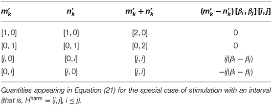
Table 1. Context-derived heterogeneous functions of monocyte subsets.

Further, it can be shown that the frequencies above also grow (in absolute value) with the inharmonicity of the interval, the other factor in perception of musical tension considered here. Let f₁ and f₂ denote the lower and the higher frequency of the interval, respectively, that is,

$\begin{array}{l}{f}_1=(1+{\beta }_i)i,\\ f_2=(1+{\beta }_j)j=\left((1+{\beta }_i)+({\beta }_j-{\beta }_i)\right)j& (22)\end{array}$

(see Equation 12). Additionally, let

$\begin{array}{l}{f}_0=1+{\beta }_i.\end{array}$

The inharmonicity of the interval [f₁, f₂] with respect to the fundamental frequency f₀ is defined as its weighted Manhattan distance to the interval [if₀, jf₀], comprising the i-th and the j-th harmonic of f₀. The distance is weighted by the squared signal amplitudes and normalized by f₀ and the sum of the squared signal amplitudes [11]. In our particular case, the inharmonicity $I_{f_1{f}_2}^{ij}$ is equal to

$\begin{array}{l}{I}_{f_1{f}_2}^{ij}=\frac{2}{f_0}\frac{|f_{0}i-f_{0}i|{\rho }_i^2+|\left(f_0+({\beta }_j-{\beta }_i)\right)j-f_{0}j|{\rho }_j^2}{{\rho }_i^2+{\rho }_j^2}\\ =\frac{2}{f_0}\frac{j|{\beta }_j-{\beta }_i|{\rho }_j^2}{{\rho }_i^2+{\rho }_j^2}\\ \frac{f_0\left({\rho }_i^2+{\rho }_j^2\right)}{2{\rho }_j^2}I=j|{\beta }_j-{\beta }_i|.\end{array}$

Indeed, the frequencies grow (in absolute value) with the inharmonicity of the interval. Consequently, noting that A governs the stability of the fixed point solution at origin without input (ρ = 0), we conclude that, under the above assumption on B_kM, pure-tone intervals with lower relative periodicity and lower inharmonicity (i.e., those perceived as less tense) cause a higher-amplitude and slower fluctuation of the driven system eigenvalues around those of A than those with higher relative periodicity and inharmonicity (perceived as more tense).

Note that there is an ambiguity of approximation represented by a choice of i and j in Equation (22). Further, Equations (16) and (17) are far from being a global model of perception of tension even in complex tones consisting of just two harmonics; they are local in the sense that they only model perception of a particular tone with respect to a particular approximation. Last but not least, we still have to demonstrate that the above fluctuations of stability translate to features of the oscillatory dynamics in a meaningful way. We address these issues now when considering the general case of stimulation with a complex tone consisting of more than two harmonics. To this end, we construct an array of models like Equation (16) differing in eigenfrequency. Here, each eigenfrequency represents a choice of f₀ in Equation (22) so that the entire array essentially works as a pitch detector. Time traces from simulations of such an array are depicted in Figures 1, 2.

FIGURE 1

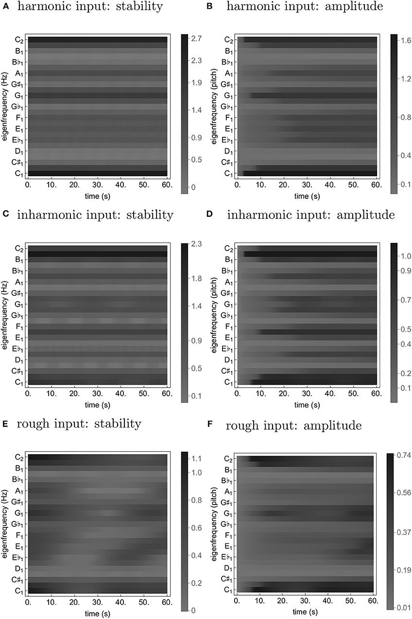
Figure 1. Time traces from simulations of Equation (24) with a soft harmonic (A,B), inharmonic (C,D), and rough (E,F) input. The stability (A,C,E) is quantified as ℜ((J)_{[0, 0]}) (see Equation 2); the amplitude (B,D,F) is simply |z_1k|.

FIGURE 2

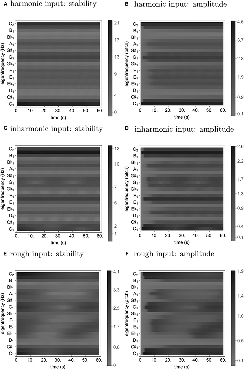
Figure 2. Time traces from simulations of Equation (24) with a loud harmonic (A,B), inharmonic (C,D), and rough (E,F) input. The stability (A,C,E) is quantified as ℜ((J)_{[0, 0]}) (see Equation 2); the amplitude (B,D,F) is simply |z_1k|.

The equations for the array were derived by applying the above restriction on linear terms to Equation (9), writing-out the inputs (Equations 12, 16, 17) and using Equations (6) and (18),

$\begin{array}{l}{\dot{z}}_1=\left(\alpha +ı+{\displaystyle \sum _{\begin{array}{c}p\Omega -q\Omega =0\\ \left|p\right|+\left|q\right|\ge 1\end{array}}{c}_{10pq}}{\rho }^{p+q}{e}^{ı(p-q)\phi }{e}^{ı(p-q){\Omega }_{\beta }t}\right)z_1\hfill \\ +z_1{\left|z_1\right|}^2{{\displaystyle \sum _{k=0}^{\infty }\left|z_1\right|}}^{2k}{\displaystyle \sum _{p\Omega -q\Omega =0}{c}_{(s+1)spq}}{\rho }^{p+q}{e}^{ı(p-q)\phi }{e}^{ı(p-q){\Omega }_{\beta }t}\hfill \\ +{\displaystyle \sum _{\begin{array}{c}[r,s,p,q]\in S\\ p\Omega -q\Omega \ne 0\\ r+s\ge 2\end{array}}{c}_{rspq}}{z}_1^r{\overline{z_1}}^s{\rho }^{p+q}{e}^{-ı(r-s-1)t}{e}^{ı(p-q)\phi }{e}^{ı(p-q){\Omega }_{\beta }t},\hfill & (23)\end{array}$

then truncating the higher-order terms,

$\begin{array}{c}{\dot{z}}_1=\left(\alpha +ı+{\displaystyle \sum _{\begin{array}{c}p\Omega -q\Omega =0\\ p={({\omega }_j)}_i,q={({\omega }_i)}_j\end{array}}{c}_{10pq}}{\rho }^{p+q}{e}^{ı(p-q)\phi }{e}^{ı(p-q){\Omega }_{\beta }t}\right)z_1\\ +c_{2100}{z}_1{\left|z_1\right|}^2,\end{array}$

and, finally, setting

$\begin{array}{l}{c}_{2100}=-1,c_{10pq}=1,\phi =0,z_1=z_{1k},\rho ={\rho }_k,\end{array}$

and scaling the time for convenience by the eigenfrequency, f_k, which yields a parametrically-forced normal form for supercritical Andronov-Hopf bifurcation:

$\begin{array}{ll}{\dot{z}}_{1k}=f_k\left(\left(\alpha +ı+{\displaystyle \sum _{\begin{array}{c}p\Omega -q\Omega =0\\ p={({\omega }_j)}_i,q={({\omega }_i)}_j\end{array}}{\rho }_k^{p+q}}{e}^{ı(p-q){\Omega }_{\beta }t}\right)z_{1k}-z_{1k}{\left|z_{1k}\right|}^2\right).& (24)\end{array}$

Here, (ω_j)_i signifies a vector with ω_j at the i-th position and zero otherwise. Ω and β are set as

$\begin{array}{l}\Omega =\left[{\omega }_1,{\omega }_2,\dots ,{\omega }_{54}\right]=\left[1,1,\dots ,1,2,2,\dots ,2,\dots ,6,6,\dots ,6\right]\\ \beta ={\Omega }_{24TET}\frac{1}{\Omega }-1\end{array}$

(see Equations 1, 8), where each element of Ω_24TET approximates the corresponding element of Ω as a power of $2^{\frac{1}{24}}$ (the 24-tone equal-tempered tuning); Ω and Ω_24TET are aligned in such a way that ω₅ = ω_{24TET, 5} = 1 and hence β₅ = 0. The oscillators (Equation 24) receive connections from a bank of input units—linear oscillators with eigenfrequencies spanning from B♭₀ to B₄ in quarter-tone steps. In accordance with Equation (8), each oscillator (Equation 24) is only connected to input units with frequencies (f_kω_iβ_i in Equation 8, after scaling by f_k) approximating its harmonics (in the above tuning) and, additionally, to frequencies up to 4 quarter-tones below and above these. In other words, it does not have fixed homogeneous connectivity input strength from all input units, but rather receives (weighted) input only from input units with frequencies close to its first six approximate harmonics; the connectivity of each oscillator is thus effectively defined by a connectivity pattern or kernel consisting of six unimodal elementary Gaussian kernels (k(l) = e^−0.5l2; l ∈ {−4, …, 4} and k(l) = 0 otherwise) centered at the harmonics. See visualization of the connectivity kernel in Figure 3. Moreover, only the connections emanating from the input units whose frequencies are included in the stimulus are set to have nonzero amplitude in the respective simulation. Note that by fixing a set of eigenfrequencies (corresponding to different choices of f₀ in Equation 22) and input units and restricting the connectivity to (near-)harmonics, there remains no ambiguity in approximation of the input; each oscillator, as long as the input falls within the reach of its connectivity kernel, approximates the input in its own, unique, way.

FIGURE 3

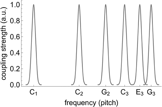
Figure 3. Connectivity of the oscillator with eigenfrequency C₁ (k = 1, see Equation 24). The first “blob” represents connections which stem from input units with eigenfrequencies ranging from B♭₀ to D₁ and target the oscillator's “slots” corresponding to ρ_1,1, ρ_1,2, …, ρ_1,9 in Equation (24); likewise, the second blob connects B♭₁, …, D₂ to ρ_1,10, ρ_1,11, …, ρ_1,18 etc. The connectivity of any other oscillator is obtained by shifting this kernel so that the center of the first blob is aligned with the oscillator's eigenfrequency.

All simulations were run from initial conditions

$\begin{array}{l}{z}_{1k}(t_0=0)=0.001,\end{array}$

with

$\begin{array}{l}\alpha =-0.001,\end{array}$

a parameter setting corresponding to the (almost loss of) stability (without input) of the fixed point z_1k = 0. Three alternative inputs were applied, whose spectra can be seen in Figure 4. The first corresponds to harmonic input with the C tone at its base plus its first five harmonics (tones with integer multiple frequencies of the base tone). The second input results from a transformation of the first which increases inharmonicity while the third is a result of a transformation which increases roughness.

FIGURE 4

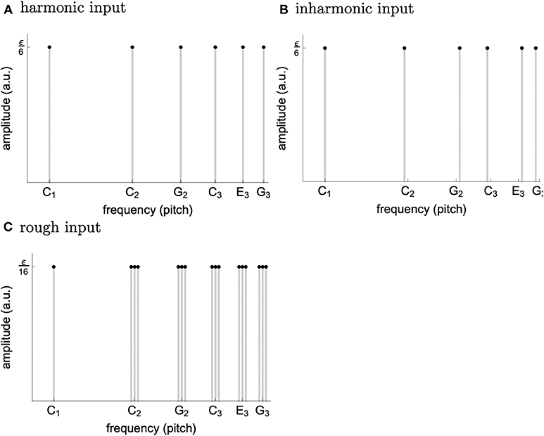
Figure 4. Spectrum of the harmonic (A), inharmonic (B), and rough (C) input used in the simulations. The construction loosely follows the procedure from [11]. We chose ϵ = 3 for the soft and ϵ = 5.4 for the loud inputs.

As can be seen from Figures 1, 2, both transformations seem to increase fluctuation of stability of the origin, as predicted by our analysis pertaining to two-frequency stimulation. This results in an increase in amplitude modulation across the oscillator array and a corresponding decrease in peak amplitude (see Figure 5). In other words, an increase in perceived musical tension seems to be related to an increase in fluctuation of stability of the origin which manifests itself as an absence of a stable dominant amplitude peak. These preliminary observations are largely confirmed by computing the minimum and the maximum of each oscillator's amplitude trace (see Figure 6). Consequently, we put forward the absence of a stable dominant amplitude peak as a hallmark of perceived musical tension in our model.

FIGURE 5

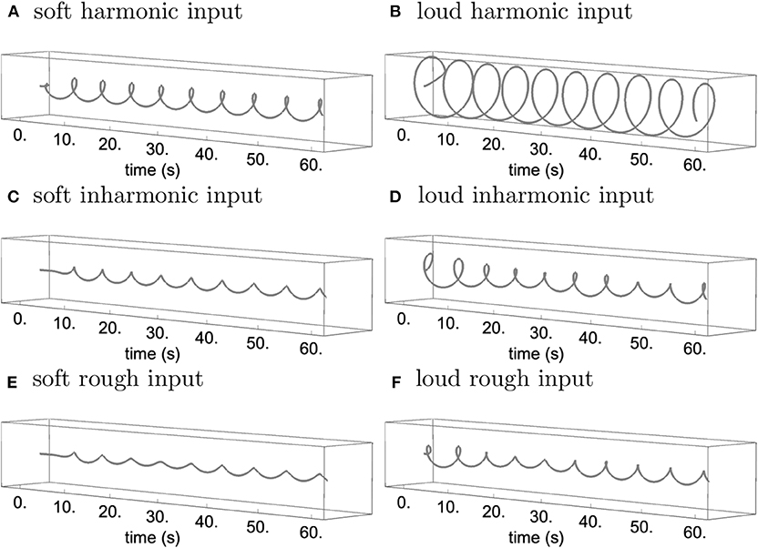
Figure 5. Trajectory of the C₁ oscillator with soft/low-amplitude input corresponding to Figure 1 (A,C,E) and loud/high-amplitude input corresponding to Figure 2 (B,D,F) for the harmonic (A,B), inharmonic (C,D), and rough input (E,F), rendered in the complex plane.

FIGURE 6

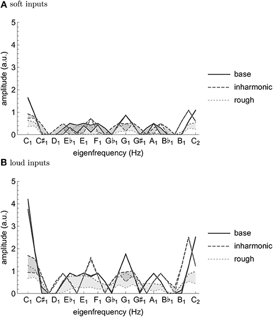
Figure 6. Minima and maxima of the oscillator amplitude traces from simulations with soft/low-amplitude input corresponding to Figure 1 (A) and loud/high-amplitude input corresponding to Figure 2 (B) with the first 20 s dropped to attenuate the effect of the same initial conditions. Incidentally, note the similarities between Figure 6 and the major key profile from Krumhansl and Kessler [32].

4. Discussion

We propose the absence of a stable unambiguous pitch detection modeled as the absence of a pronounced amplitude peak in an array of oscillators to be a correlate of timbre-induced musical tension. In the class of oscillators we chose for populating the array, the amplitude of the limit cycle is determined by the stability of the origin; if the stability switches between a stable and an unstable regime fast enough, the amplitude doesn't have enough time to grow. We show that the frequency and magnitude of this switching depends on inharmonicity and roughness of the input to the oscillator. Imagine such an oscillator is actually present in the brain; when subject to a tense (inharmonic and/or rough) stimulus, it will remain almost silent, leading to an “unclear,” “unstable,” “difficult to memorize” etc. percept (see Figures 1, 2D,F). In contrast, a less tense stimulus would result in a “clear”, “stable”, “easy to memorize” etc. percept (see Figures 1, 2B). Of course, neurophysiological and neuroimaging evidence shows the what we have in our head is not a single oscillator, but rather an entire bank of them; we show in our simulations that the results of our analysis of single oscillator generalize to an array of them in the sense that the average oscillation amplitude across the array is lower for tense than less tense stimuli (see Figure 6).

Of course, tension is clearly not a one-dimensional phenomenon and different aspects of it could be related to different aspects of the underlying neurodynamics. For instance, in a nonlinear model like the one proposed here, loudness of the input is going to affect both the general amplitude of the oscillations and their temporal fluctuations—in a frequency-dependent manner, as our example simulations for two loudness levels suggest. We consider disentangling these not necessarily orthogonal dimensions of tension as a natural extension of the currently proposed modeling framework.

We have proposed a neurodynamical model of musical tension (see Equation 24) which reproduces existing empirical results on timbral correlates of tension, is consistent with neuroimaging findings [14] in that consonant stimuli compared to dissonant stimuli elicit more sustained periodic neuronal activity of higher amplitude, and due to its generative nature can provide prediction of perceived tension of an arbitrary sound input. More precisely, we have demonstrated that both inharmonicity and roughness make the spectrum of the simulated signal flatter and more variable (wider range over time) (see Figures 1, 2, 6). Note that while [14] quantified the periodicity by the amplitude of the autocorrelation peak of the signal spectra, we rather proposed the absence of a temporally persistent, pronounced amplitude peak in the spectrum of the elicited neural activity as a possible correlate of tension—a related indicator that is also present in the results presented in [14]. One might even speculate, based on the similarity of the spectrum to the major key profile [32], that the same principles underlie perception of tonality.

Considering the simulation results reported above in more detail, we note that the overall increase in fluctuation of stability of the origin for the inharmonic and the rough input as compared to the harmonic one can be explained based on the analytical insights into the dynamics of a single oscillator obtained earlier. More precisely, the nearly-harmonic relations in the inharmonic and the rough input introduce oscillating terms into most of the oscillators' coupling functions; the increase of amplitude modulation is, in turn, accounted for by the fact that the amplitude of the stable limit cycle of Equation (24) is determined by the stability of the origin. The decrease of the peak amplitude is, for the inharmonic input, probably due to the connectivity; there are no exact harmonic relations in the input and hence no oscillator can align its connectivity kernel optimally with the input (see Figure 3). For the rough input, it might be a consequence of scaling down the amplitudes of its frequency components to keep the overall loudness equal to that of the other inputs which consist of fewer harmonics (see Figure 4).

As for our general approach, a few comments are in order. First, for the sake of simplicity, we chose a subclass of multiple centers [a generalization of double centers; see [26]] as our family of models. It might be an interesting avenue for future research to determine whether there are other families of models in which relative periodicity and inharmonicity of the input plays such an important role.

Also for the sake of simplicity, we only considered relative periodicity and inharmonicity of pure-tone dyads. For general sounds, we would be dealing with the set of nonnegative solutions to a general linear Diophantine equation (Equation 18). To the best of our knowledge, the structure of the set (its minimum generators) can only be determined algorithmically [e.g., [31]]. This makes analytical insights virtually impossible in the general case.

Further, concerning the phenomenon wherein loud music is perceived as more tense than soft music [8], we argue that, replacing the bank of input units with a model of cochlea, the effective input generated by a loud harmonic spectrum would be very similar to the rough input used in the simulations reported here. More precisely, we expect the loud harmonic spectrum to displace not only those segments of the basilar membrane whose eigenfrequencies match the harmonics, but also the adjacent segments (see Figure 4). This way, the effect of loudness would be accounted for by a combination of cochlear physiology and sensitivity of our model to roughness.

Finally, even though the choice of spectral representation was motivated by our interest in contemporary art music, especially the so-called “spectral music,” the model presented here is applicable to any kind of music; indeed, even music composed with traditional categories in mind ends up being rendered as sound which can be fed into our model.

To conclude, mapping perception to neurodynamics is hard. However, from time to time, a favorable constellation of research sheds light on the underlying physiology. The fruitful concept of relative periodicity [13] suggests that roughness, as one of the perceptual “dimensions” of timbre contributing to tension, might originate in (neural) resonance. Indeed, in this study, we have shown that the dynamics of stability of the origin in a wide class of periodically forced nonlinear oscillators crucially depends on the relative periodicity of the input and, additionally, on its inharmonicity. Since roughness and inharmonicity are principal constituents of perceived tension, we have effectively put forward a possible neurodynamical explanation of musical tension. Moreover, for a particular model belonging to the above class, we have demonstrated by simulations that tense inputs result in an absence of a persistent dominant peak in the spectrum of the time series generated by the model.

Data Availability Statement

The datasets generated for this study are available on request to the corresponding author.

Author Contributions

JH and MH contributed to conception, theoretical analysis, design of the study, manuscript revision, read and approved the submitted version. MH implemented the simulations and visualizations and wrote the first draft of the manuscript.

Funding

This study was funded by the project Nr. LO1611 with a financial support from the MEYS under the NPU I program and with institutional support RVO:67985807.

Conflict of Interest

The authors declare that the research was conducted in the absence of any commercial or financial relationships that could be construed as a potential conflict of interest.

Acknowledgments

We thank Pavel Sanda and Hana Markova for reading the manuscript and providing helpful comments.

References

1. Anderson W, Mathiesen TJ. Ethos. Oxford University Press (2001). Available online at: http://www.oxfordmusiconline.com/subscriber/article/grove/music/09055

Google Scholar

2. Huron D. Sweet Anticipation. Cambridge, MA: The MIT Press (2006).

Google Scholar

3. Aldwell E, Schachter C, Cadwallader A. Harmony & Voice Leading. Exeter: Schirmer Cengage Learning (2011).

Google Scholar

4. Lerdahl F, Krumhansl CL. Modeling tonal tension. Music Percept. (2007) 24:329–66. doi: 10.1525/mp.2007.24.4.329

CrossRef Full Text | Google Scholar

5. Murail T. The revolution of complex sounds. Contemp Music Rev. (2005) 24:121–35. doi: 10.1080/07494460500154780

CrossRef Full Text | Google Scholar

6. Murail T. Target practice. Contemp Music Rev. (2005) 24:149–71. doi: 10.1080/07494460500154814

CrossRef Full Text | Google Scholar

7. Fineberg J. Spectral music. Contemp Music Rev. (2000) 19:1–5. doi: 10.1080/07494460000640221

CrossRef Full Text | Google Scholar

8. Ilie G, Thompson WF. A comparison of acoustic cues in music and speech for three dimensions of affect. Music Percept. (2006) 23:319–30. doi: 10.1525/mp.2006.23.4.319

CrossRef Full Text | Google Scholar

9. Bigand E, Parncutt R, Lerdahl F. Perception of musical tension in short chord sequences: the influence of harmonic function, sensory dissonance, horizontal motion, and musical training. Percept Psychophys. (1996) 58:125–41. doi: 10.3758/BF03205482

PubMed Abstract | CrossRef Full Text | Google Scholar

10. Pressnitzer D, McAdams S, Winsberg S, Fineberg J. Perception of musical tension for nontonal orchestral timbres and its relation to psychoacoustic roughness. Percept Psychophys. (2000) 62:66–80. doi: 10.3758/BF03212061

PubMed Abstract | CrossRef Full Text | Google Scholar

11. Farbood MM, Price KC. The contribution of timbre attributes to musical tension. J Acoust Soc Am. (2017) 141:419–27. doi: 10.1121/1.4973568

PubMed Abstract | CrossRef Full Text | Google Scholar

12. Hutchinson W, Knopoff L. The acoustic component of Western consonance. J New Music Res. (1978) 7:1–29. doi: 10.1080/09298217808570246

CrossRef Full Text | Google Scholar

13. Stolzenburg F. Harmony perception by periodicity detection. J Math Music. (2015) 9:215–38. doi: 10.1080/17459737.2015.1033024

CrossRef Full Text | Google Scholar

14. Lee KM, Skoe E, Kraus N, Ashley R. Neural transformation of dissonant intervals in the auditory brainstem. Music Percept. (2015) 32:445–59. doi: 10.1525/mp.2015.32.5.445

CrossRef Full Text | Google Scholar

15. Bidlack RA. Music From Chaos: Nonlinear Dynamical Systems as Generators of Musical Materials. San Diego, CA: University of California (1990).

Google Scholar

16. Boon JP, Decroly O. Dynamical systems theory for music dynamics. Chaos. (1995) 5:501–8. doi: 10.1063/1.166145

PubMed Abstract | CrossRef Full Text | Google Scholar

17. Hennig H, Fleischmann R, Fredebohm A, Hagmayer Y, Nagler J, Witt A, et al. The nature and perception of fluctuations in human musical rhythms. PLoS ONE. (2011) 6:e26457. doi: 10.1371/journal.pone.0026457

PubMed Abstract | CrossRef Full Text | Google Scholar

18. Coombes S, Lord GJ. Intrinsic modulation of pulse-coupled integrate-and-fire neurons. Phys Rev E. (1997) 56:5809. doi: 10.1103/PhysRevE.56.5809

CrossRef Full Text | Google Scholar

19. Lots IS, Stone L. Perception of musical consonance and dissonance. J R Soc Interface. (2008) 5:1429–34. doi: 10.1098/rsif.2008.0143

PubMed Abstract | CrossRef Full Text | Google Scholar

20. Heffernan B, Longtin A. Pulse-coupled neuron models as investigative tools for musical consonance. J Neurosci Methods. (2009) 183:95–106. doi: 10.1016/j.jneumeth.2009.06.041

PubMed Abstract | CrossRef Full Text | Google Scholar

21. Ushakov YV, Dubkov AA, Spagnolo B. Spike train statistics for consonant and dissonant musical accords in a simple auditory sensory model. Phys Rev E. (2010) 81:041911. doi: 10.1103/PhysRevE.81.041911

PubMed Abstract | CrossRef Full Text | Google Scholar

22. Large EW, Almonte FV, Velasco MJ. A canonical model for gradient frequency neural networks. Phys D. (2010) 239:905–11. doi: 10.1016/j.physd.2009.11.015

PubMed Abstract | CrossRef Full Text | Google Scholar

23. Large EW. A Dynamical systems approach to musical tonality. In: Huys R, Jirsa VK, editors. Nonlinear Dynamics in Human Behavior. Vol. 328 of Studies in Computational Intelligence. Berlin; Heidelberg: Springer (2011). p. 193–211. doi: 10.1007/978-3-642-16262-6_9

CrossRef Full Text | Google Scholar

24. Large EW, Almonte FV. Neurodynamics, tonality, and the auditory brainstem response. Ann NY Acad Sci. (2012) 1252:E1–7. doi: 10.1111/j.1749-6632.2012.06594.x

PubMed Abstract | CrossRef Full Text | Google Scholar

25. Large EW, Kim JC, Flaig NK, Bharucha JJ, Krumhansl CL. A neurodynamic account of musical tonality. Music Percept. (2016) 33:319–31. doi: 10.1525/mp.2016.33.3.319

CrossRef Full Text | Google Scholar

26. Murdock J. Normal Forms and Unfoldings for Local Dynamical Systems. New York, NY: Springer-Verlag (2003). doi: 10.1007/b97515

CrossRef Full Text | Google Scholar

27. Lerud KD, Almonte FV, Kim JC, Large EW. Mode-locking neurodynamics predict human auditory brainstem responses to musical intervals. Hear Res. (2014) 308:41–9. doi: 10.1016/j.heares.2013.09.010

PubMed Abstract | CrossRef Full Text | Google Scholar

28. Kim JC, Large EW. Signal processing in periodically forced gradient frequency neural networks. Front Comput Neurosci. (2015) 9:152. doi: 10.3389/fncom.2015.00152

PubMed Abstract | CrossRef Full Text | Google Scholar

29. Kim JC, Large EW. Mode locking in periodically forced gradient frequency neural networks. Phys Rev E. (2019) 99:022421. doi: 10.1103/PhysRevE.99.022421

PubMed Abstract | CrossRef Full Text | Google Scholar

30. Parncutt R. Template-matching models of musical pitch and rhythm perception. J New Music Res. (1994) 23:145–67. doi: 10.1080/09298219408570653

CrossRef Full Text | Google Scholar

31. Clausen M, Fortenbacher A. Efficient solution of linear diophantine equations. J Symbol Comput. (1989) 8:201–16. doi: 10.1016/S0747-7171(89)80025-2

CrossRef Full Text | Google Scholar

32. Krumhansl CL, Kessler EJ. Tracing the dynamic changes in perceived tonal organization in a spatial representation of musical keys. Psychol Rev. (1982) 89:334. doi: 10.1037/0033-295X.89.4.334

PubMed Abstract | CrossRef Full Text | Google Scholar