Analog Image Modeling for 3D Single Image Super Resolution and Pansharpening

1. Introduction

During image acquisition, we often loose resolution due to the limited density of the imaging sensors and the blurring of the acquisition lens. Image super resolution, a post process to increase image resolution, is an efficient way to achieve a resolution beyond what the hardware offers. A detailed overview of this area is outlined in Farsiu et al. [1], Yang et al. [2], and Park et al. [3]. Current techniques of solving this ill-posed problem are often insufficient for many real world applications [4, 5]. We propose an analog modeling based three-dimensional (3D) color image super resolution and pansharpening method.

In recent literature, image super-resolution (SR) methods typically fall into three categories: interpolation based methods, learning based methods, and constrained reconstruction methods. Interpolation based methods [6, 7] such as nearest-neighbor, bilinear and bicubic interpolation use analytical priors to recover a continuous-time signal from the discrete pixels. They work very well for smooth regions and are simple to compute. In dictionary learning based models, the missing high frequency detail is recovered from a sparse linear combination of dictionary atoms trained from patches of the given low-resolution (LR) image [8, 9] or from an external database of patches [10–12]. Dictionary learning based methods explore the self-similarities of the image and are robust, albeit rather slow training time of the dictionary atoms. Models based on constrained reconstruction use the underlying nature of the LR image to define prior constraints for the target HR image. Sharper structures can be recovered using these models. Priors common to these techniques include total variation priors [13–15], gradient priors [16, 17] and priors based on edge statistics [18]. The proposed method falls in this category. Another category is deep neural network based approach that uses a large amount of training data to obtain super results [19–22].

Increased accessibility to satellite data has led to a wide range of applications in multispectral (MS) SR. These applications include target detection, scene classification, and change detection. A multitude of algorithms have been presented in recent literature to address this task. However, the performance of many of these algorithms are data dependent with respect to existing quantitative assessment measures. With the increasing advancements in technology, there have been varying modes of image acquisition systems. In remote sensing, satellites carry sensors that acquire images of a scene in multiple channels across the electromagnetic spectrum. This gives rise to what is referred to as multispectral imaging. Due to high cost overheads in developing sensors that can faithfully acquire scene data with high spectral and spatial resolution, the spatial resolution in the data acquisition process is often compromised. The low-spatial resolution MS images usually consist of images across 4–8 spectral bands: red, green, blue, as well as near infrared bands (provide Landsat, IKONOS, etc. specifications).

Most satellites also acquire a high-spatial resolution image known as a panchromatic image. The technique of using panchromatic (PAN) to compensate for the reduction in spatial-resolution of the MS images is referred to as pansharpening. The success of pansharpening relies on the extent one can explore the structural similarity between the PAN and the high-resolution (HR) MS image [23]. In recent years, pansharpening methods fall under three main categories: component substitituion (CS), multiresolution analysis (MRA), and variational methods. Detailed surveys can be found in Loncan et al. [24] and Vivone et al. [25].

The main assumption of CS methods is that the spatial and spectral information of the high spectral resolution image can be separated in some space [24]. Examples of CS methods include principal component analysis (PCA) [26, 27], intensity-hue-saturation (IHS) methods [28–30], Brovey method [31], and Gram-Schmidt (GS) based methods [32]. These methods enhance the spatial resolution of the LR MS image at the expense of some loss in the spectral detail. Compared to the CS methods, MRA methods have better temporal coherence between the PAN and the enhanced MS image. MRA methods yield results with better spectral consistency at the expense of designing complex filters to mimic the reduction in the resolution by the sensors. Spatial details are injected into the MS data after a multi-scale decomposition of the PAN [24]. Examples of MRA methods include high-pass filtering (HPF) [30], smooth filter-based intensity modulation (SFIM) [33], generalized Laplacian pyramid (GLP) methods [34, 35], additive “á trous” wavelet transform (ATWT) methods [23, 36] and additive wavelet luminance proportional (AWLP) [37]. Variational methods are more robust compared to the CS and MRA techniques, albeit rather slow in comparison [24]. A common tool used by these approaches is regularization. This is used to promote some structural similarity between the LR MS, HR MS, and PAN images [24, 38, 39]. Among these methods include models based on the Bayesian framework and matrix factorization methods [24, 38, 39].

In this paper, we extend the key ideas in the SR model in Deng et al. [40] to 3D framework. We then test the performance of the model with single image super-resolution and pansharpening.

1.1. Related Work

In Deng et al. [40], a 2D image defined on a continuous domain [0, 1] × [0, 1] is assumed to have a density function that is the sum of two parts, reproducing kernel Hilbert space (RKHS) and Heaviside functions to study single image super-resolution (SISR) whereby the problem is cast as an image intensity function estimation problem. They assume that the smooth components of the image belong to a special Hilbert space called RKHS, and can be spanned by a basis based on an approximation by spline interpolation [41]. The Heaviside function is used to model the edges and discontinuous information in the input image. Using a patch-based approach, the intensity information of the LR input image patches are defined on a coarser grid to estimate the coefficients of the basis functions. To obtain the enhanced resolution result, they utilize the obtained coefficients and an approximation of the basis functions on a finer grid. Furthermore, to recover more high frequency information the authors employ an iterative back projection method [42] after the HR image has been obtained. Color images were tested in Deng et al. [40], however the analog modeling was done the luminance channel only after transforming the color space. This RKHS+Heaviside method is extended to pansharpening in Deng et al. [43]. In the pansharpening framework the different bands share the same basis but with different coefficients patch by patch, and channel by channel. A panchromatic image is used to guide the model and it is assumed to be a linear combination of the multiple bands.

1.2. Contribution

Using the same basis as in Deng et al. [40], we present a three-dimensional SR algorithm for true color images based on continuous/analog modeling. We also extend it to pansharpening. Instead of estimating the basis coefficients patch by patch and band by band, we cluster patches and conduct computation cluster by cluster. Similarity of patches within one cluster leads to some natural regularity. We jointly optimize all the coefficients for all the bands of the model rather than optimizing for each independent band. Furthermore, we use clustering techniques to improve the structural coherence of the desired results in the optimization model. Spatially, we divide the images into small overlapping patches and cluster these patches classes using k-means clustering. To improve the spectral coherence of the results, we cluster the image bands into groups based on correlation statistics and the perform the optimization on each of the groups obtained.

In this paper, we use the RKHS approximations to model the smooth components of the image whiles preserving the non-smooth components by the approximated Heaviside function. For the pansharpening experiments, We also preprocess the data using fast state-of-the-art MRA techniques [37] to incorporate some similarity in the spectral channels of the fused image. Thus we develop a continuous 3D modeling framework for multispectral pansharpening.

The experiments that follow show that these contributions yield better enhanced resolution results with faster convergence speeds at all scales.

The paper is organized as follows. In section 2, we review the regular functions used in decomposing the image. The proposed model is described in section 3 with numerical results outlined in section 4.

2. Background Review

In this section, we review the mathematical functions used in the formulation of our model. Similar as in Deng et al. [40], we model image intensity function defined on a small image patch as a linear combination of reproducing Kernel Hilbert function (RKHS) and approximated Heaviside function (AHF) which models the smooth and edge components, respectively.

2.1. Reproducible Kernel Hilbert Spaces

RKHS can be used to define feature spaces to help compare objects that have complex structures and are hard to distinguish in the original feature space. Wahba [41] proposed polynomial spline models for smoothing problems. Our proposed model is based on this approach using the Taylor series expansion. We review these methods in the following subsections.

2.1.1. Signal Smoothing Using Splines

Let ${G}$ represent a family of functions on [0,1] with continuous derivatives up to order (m − 1),

$\begin{array}{l}{G}=\left\{f:f\in {{C}}^{m-1}\left[0,1\right],f^{(m)}\in {{L}}_2\left[0,1\right]\right\}.\end{array}$

By Taylor's theorem with remainder for $f\in {G}$, we may write

$\begin{array}{ll}f(t)=\underset{f_0(t)}{\underbrace{{\displaystyle \sum _{\nu =0}^{m-1}\frac{t^{\nu }}{\nu !}}{f}^{(\nu )}(0)}}+\underset{f_1(t)}{\underbrace{{\displaystyle {\int }_0^1\frac{{(t-u)}_{+}^{m-1}}{(m-1)!}}{f}^{(m)}(u)du}},& (1)\end{array}$

for some u, where (x)₊ = x for x ≥ 0 and (x)₊ = 0 otherwise. Let

$\begin{array}{ll}{\varphi }_{\nu }(t)=\frac{t^{\nu -1}}{(\nu -1)!},1\le \nu \le m,& (2)\end{array}$

and ${{H}}_0=\mathrm{\text{span}}{\left\{{\varphi }_i\right\}}_{1\le i\le m}$ endowed with norm $\Vert \varphi {\Vert }^2=\sum _{\nu =0}^{m-1}{\left[(D^{\nu }\varphi )(0)\right]}^2$, then $D^{(m)}({{H}}_0)=0$, where D^m denotes the mth derivative. It can be shown that a reproducing kernel exists for ${{H}}_0$ and is defined as

$\begin{array}{ll}{R}^0(s,t)={\displaystyle \sum _{\nu =1}^m}{\varphi }_{\nu }(s){\varphi }_{\nu }(t),& (3)\end{array}$

therefore for any $f_0\in {H}$, we have $f_0(t)=\sum _{\nu =1}^m{d}_{\nu }{\varphi }_{\nu }(t).$

Let ${{B}}_m=\left\{f:f\in {{C}}^{m-1}\left[0,1\right],f^{\nu }(0)=0,\nu =0,1,\dots ,m-1\right\}$ and define

$\begin{array}{ll}{G}_m(t,u)=\frac{{(t-u)}_{+}^{m-1}}{(m-1)!}.& (4)\end{array}$

The space

$\begin{array}{l}{{H}}_1=\{f:f\in {{B}}_m,\text{ with }f,f^{\prime },\dots ,f^{(m-1)}\\ \text{ absolutely continuous},f^{(m)}\in {{L}}_2\}\end{array}$

with norm $\Vert f{\Vert }^2={\displaystyle {\int }_0^1(f^{(m)}(}t){)}^{2}dt$ can be shown to be an RKHS with reproducing kernel

$\begin{array}{ll}{R}^1(x,t)={\displaystyle {\int }_0^1}{G}_m(t,u)G_m(x,u)du,& (5)\end{array}$

so that for any $f_1\in {{H}}_1$, we have $f_1(t)=\sum _{i=1}^n{c}_i{\xi }_i,$ where ${\xi }_i(·)=R^1(s_i,·).$ It follows from the properties of the RKHS, we can construct a direct sum space ${{G}}_m={{H}}_0+{{H}}_1$ since

$\begin{array}{ll}{\displaystyle {\int }_0^1((}{D}^m{f}_0)(u){)}^{2}du=0,{\displaystyle \sum _{\nu =0}^{m-1}(}{D}^{(\nu )}{f}_1(0){)}^2=0.& (6)\end{array}$

The reproducing kernel for ${{G}}_m$ can be shown [41] to be

$\begin{array}{ll}R(s,t)=R^0(s,t)+R^1(s,t),& (7)\end{array}$

with norm

$\begin{array}{ll}\Vert f{\Vert }^2={\displaystyle \sum _{\nu =0}^{m-1}}{[(D^{\nu }f)(0)]}^2+{\displaystyle {\int }_0^1}{(f^{(m)}(t))}^{2}dt,f\in {{G}}_m,& (8)\end{array}$

therefore for any $f\in {{G}}_m$, we have f = f₀ + f₁ with $f_0\in {{H}}_0,f_1\in {{H}}_1$ and

$\begin{array}{ll}f(t)={\displaystyle \sum _{\nu =1}^m}{d}_{\nu }{\varphi }_{\nu }(t)+{\displaystyle \sum _{i=1}^n}{c}_i{\xi }_i,t\in \left[0,1\right].& (9)\end{array}$

Let $d={(d_1,\dots d_m)}^T$ and $c={(c_1,\dots ,c_n)}^T$ be coefficient vectors, $f={\left(f(t_1),\mathrm{...},f(t_p)\right)}^T$ represent the discretization of f on discrete grids $t_j,j=1,2,\cdots n_t,T\in {ℝ}^{n\times m},\Sigma \in {ℝ}^{n\times n}$ with T_jν = ϕ_ν(t_j), Σ_ji = ξ_i(t_j), then f = Td + Σc. Given the observation data

$\begin{array}{ll}g=f+\eta & (10)\end{array}$

where η denotes additive Gaussian noise. To find f from g, we need to estimate the coefficients d and c. Following Wahba [41], the coefficients d, c are estimated from the discrete measurements g by

$\begin{array}{ll}(c,d)=\text{arg min}\left\{\frac{1}{n}\Vert g-Td-\Sigma c{\Vert }^2+\mu c^T\Sigma c\right\},& (11)\end{array}$

where the term μc^TΣc is a non-smoothness penalty. Closed form solutions for c and d can be obtained. The parameter m controls the total degree of the polynomials used to define T. For example, when m = 3 the basis functions are given as ϕ₁(x) = 1, ϕ₂(x) = x and ${\varphi }_3(x)=x^2/2$.

2.1.2. Image Smoothing Using Splines

Extending the one-dimensional spline model to two-dimensional data, we consider a similar discretization and set up a model similar to that defined in (11). Let $f={\left(f(t_1),\dots ,f(t_{n_t})\right)}^T$, t_i ∈ [0, 1] × [0, 1] be a discretization for an observed noisy image. From Wahba [41], an estimate of f can be obtained from the additive noise data model in (10) for images by minimizing the following

$\begin{array}{ll}\text{min}\left\{\frac{1}{n}\Vert g-f{\Vert }_2^2+\mu J_m(f)\right\}& (12)\end{array}$

where m defines the order of the partial derivatives in ${{L}}_2([0,1]\times [0,1])$, and with the penalty function defined by

$\begin{array}{ll}{J}_m(f)={\displaystyle \sum _{\nu =0}^m{\displaystyle {\int }_0^1{\displaystyle {\int }_0^1\left(\begin{array}{c}m\\ \nu \end{array}\right)}}}{\left(\frac{{\partial }^{m}f}{\partial x^{\nu }\partial y^{m-\nu }}\right)}^{2}dxdy.& (13)\end{array}$

The null space of J_m is the $M=\left(\begin{array}{c}2+m-1\\ 2\end{array}\right)$-dimensional space spanned by polynomials in two variables with total degree at most m − 1. In this paper, and we choose m = 3 so that M = 6 and the null space of J_m is spanned by monomials ϕ₁, ϕ₂, …, ϕ₆ given by

$\begin{array}{l}\begin{array}{c}{\varphi }_1(x,y)=1,{\varphi }_2(x,y)=x,{\varphi }_3(x,y)=y,\\ {\varphi }_4(x,y)=xy,{\varphi }_5(x,y)=x^2,\text{and }{\varphi }_6(x,y)=y^2.\end{array}\end{array}$

Duchon [44] proved that a unique minimizer f_μ exists for (12) with representation

$\begin{array}{ll}{f}_{\mu }(t)={\displaystyle \sum _{\nu =1}^M}{d}_{\nu }{\varphi }_{\nu }(t)+{\displaystyle \sum _{i=1}^n}{c}_i{E}_m(t,t_i),t\in \left[0,1\right]\times \left[0,1\right],& (14)\end{array}$

where E_m is defined as

$\begin{array}{ll}{E}_m(s,t)=E_m(|s-t|)={\theta }_{m,d}|s-t{|}^{2m-d}\text{ln}|s-t|,& (15)\end{array}$

and ${\theta }_{m,d}=\frac{{(-1)}^{d/2+m+1}}{2^{2m-1}{\pi }^{d/2}(m-1)!(m-d/2)!}$.

Based on the work of Duchon [44] and Meinguet [45] we can rewrite (12) to find minimizers c and d by

$\begin{array}{ll}(c,d)=\text{arg min}\left\{\Vert g-Td-Kc{\Vert }^2+\mu c^{T}Kc\right\},& (16)\end{array}$

where $T\in {ℝ}^{n_t\times M}$, with T_{i, ν} = ϕ_ν(t_i) and $K\in {ℝ}^{n_t\times n_t}$ with K_{i, j} = E_m(t_i, t_j). E_m(s, t) is the two-dimensional equivalent of ξ_i(t) in the one-dimensional case. After obtaining the coefficients, we compute f using the relationship f = Td + Kc.

2.2. Approximated Heaviside Function

The one-dimensional Heaviside step function is defined as

$\begin{array}{ll}\varphi (x)=\{\begin{array}{cc}0& x<0,\\ 1& x\ge 0\end{array}& (17)\end{array}$

Due to the singularity at x = 0, we approximate ϕ by,

$\begin{array}{ll}\psi (x)=\frac{1}{2}+\frac{1}{\pi }\text{arctan}\left(\frac{x}{\epsilon }\right),\epsilon \in ℝ& (18)\end{array}$

We refer to this as the approximated Heaviside function (AHF), an approximation to ϕ(x) as ε → 0. The variable ε controls the smoothness of the approximation [40]. A two-dimensional variation of the AHF is given by

$\begin{array}{ll}\Psi (x,y)=\psi \left(\left(\begin{array}{c}\text{cos }\theta \\ \text{sin }\theta \end{array}\right)·\left(\begin{array}{c}x\\ y\end{array}\right)+c\right)& (19)\end{array}$

with variables θ and c determining the rotations and locations of the edges as shown in Figure 1, we show the 2D and 3D surface view of the AHF at two different pairs of θ and c. Kainen et al. [46] proved that a function $f\in {{L}}_2(\left[0,1\right]\times \left[0,1\right])$ can be approximately represented by the weighted linear combination of approximated Heaviside functions:

$\begin{array}{ll}f(x,y)={\displaystyle \sum _{j=1}^{n_{\theta }}}{w}_j\psi \left(\left(\begin{array}{c}\text{cos }{\theta }_j\\ \text{sin }{\theta }_j\end{array}\right)·\left(\begin{array}{c}x\\ y\end{array}\right)+c_j\right).& (20)\end{array}$

FIGURE 1

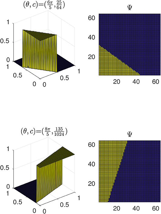
Figure 1. Illustrating the surfaces corresponding to the approximated Heaviside functions for varying pairs of θ and c.

We define $\text{Ψ}\in {ℝ}^{n_t\times n_{\theta }}$ with ${\Psi }_{i,j}=\psi \left(\left(\begin{array}{c}\cos {\theta }_j\\ \sin {\theta }_j\end{array}\right)·\left(\begin{array}{c}{x}_i\\ y_i\end{array}\right)+c_j\right),t_i=(x_i,y_i),\text{and\hspace{0.17em}}{n}_{\theta }$ is the number of rotations considered. Suppose f, g are the vectorized high and low resolution discretizations of f, respectively. The vectorized high resolution image $f\in {ℝ}^{n_1{n}_2}$ can be obtained by $f_i=f(t_i^h)$ with $t_i^h=(x_i^h,y_i^h)$, $x_i^h\in \{0,\frac{1}{n_1-1},\frac{2}{n_2-1},\dots ,1\}$, $y_i^h\in \{0,\frac{1}{n_2-1},\frac{2}{n_2-1},\dots ,1\}$ on a finer grid. Similarly, vectorized the low-resolution discretization $g\in {ℝ}^{m_1{m}_2}$ can be obtained by $g_i=f(t_i^{\ell })$ with $t_i^{\ell }=(x_i^{\ell },y_i^{\ell })$, $x_i^{\ell }\in \{0,\frac{1}{m_1-1},\frac{2}{m_1-1},\dots ,1\}$, and $y_i^{\ell }\in \{0,\frac{1}{m_2-1},\frac{2}{m_2-1},\dots ,1\}$ on a coarse grid. Now, assuming that the underlying analog image intensity function is approximated by the sum of a RKHS function and the variations of AHF with $T^{\ell }\in {ℝ}^{m_1{m}_2\times M}$, $K^{\ell }\in {ℝ}^{m_1{m}_2\times m_1{m}_2}$, and ${\text{Ψ}}^{\ell }\in {ℝ}^{m_1{m}_2\times n_{\theta }}$, we have

$\begin{array}{ll}g=T^{\ell }d+K^{\ell }c+{\text{Ψ}}^{\ell }e.& (21)\end{array}$

Thus, given the low resolution input g, the coefficient vectors $c\in {ℝ}^{m_1{m}_2}$, d∈ℝ^M and $e\in {ℝ}^{n_{\theta }}$ for the residual, smooth and edge components are obtained by solving the following minimization problem:

$\begin{array}{ll}\underset{c,d,e}{\text{min}}\left\{\Vert g-SB(T^{h}d+K^{h}c+{\Psi }^{h}e){\Vert }^2+\mu c^T{K}^{\ell }c+\gamma \Vert e{\Vert }_1\right\},& (22)\end{array}$

where B is the identity matrix in the absence of blur, S is the downsampling operator, and the superscripts h and ℓ refers to a fine and course scale matrices. The smooth components of the image are modeled by the RKHS approach, while AHF caters for the edges. Since the dictionary Ψ is pretty exhaustive, i.e., accounting for multiple edge orientations, it is reasonable to use the ||·||₁ to enforces the sparsity of as all the orientations may not be present for any given image. Once the coefficients have been obtained, we have

$\begin{array}{ll}f=T^{h}d+K^{h}c+{\text{Ψ}}^{h}e,& (23)\end{array}$

where $T^h\in {ℝ}^{n_1{n}_2\times M}$, $K^{\ell }\in {ℝ}^{n_1{n}_2\times m_1{m}_2}$, and ${\text{Ψ}}^{\ell }\in {ℝ}^{n_1{n}_2\times n_{\theta }}$. Next, we discuss our proposed model and examine some numerical experiments in the chapters that follow.

3. Proposed Models

In this section, we present our proposed models for SISR and pansharpening based on the functions defined in section 2. We propose a 3D patch-based approach that infers the HR patches from LR patches that has been grouped into classes based on their structural similarity. As a result, we impose similarity constraints within the classes so that the coefficients for neighboring patches in a group do not differ substantially. In addition, we use sparse constrained optimization techniques that simplify the minimization of the resulting energy functional by solving a series of subproblems, each with a closed form solution. Two algorithms will be discussed. The first is a 3D SR model for true color images and MS images with at most four bands. The second algorithm is an extension of our SISR model to pansharpening for MS images with at least four spectral bands. This is a two-step hybrid approach that incorporates CS and MRA methods into the first algorithm to obtain an enhanced resolution result.

3.1. Single Image Super-Resolution

Given a LR image $Y\in {ℝ}^{m_1\times m_2\times \lambda }$ we estimate the target HR image $\hat{X}\in {ℝ}^{n_1\times n_2\times \lambda }$ with n_i = ωm_i, where ω is a scale factor and λ is the number of bands as follows. We begin by decomposing the LR image into a set of overlapping patches ${{P}}_Y={\left\{Y_{p_i}\right\}}_{i=1}^{N_p}$, $Y_{p_i}\in {ℝ}^{m_p\times m_p\times \lambda }$. The size of the square patches, and the overlap between adjacent patches depend on the dimensions of the input image. We consider the use of overlapping patches to improve local consistency of the estimated image across the regions of overlap. The estimated image $\hat{X}$ will be represented by the same number of patches, N_p. Next, for a suitably chosen k, we use the k-means algorithm with careful seeding [47] to cluster the patches into k classes ${{P}}_Y^1,\dots {{P}}_Y^k$, as shown in Figure 2. In this paper, the value of k is determined empirically to obtain the best result. Clustering is done so that each high resolution patch generated preserves some relationships with its neighboring patches.

FIGURE 2

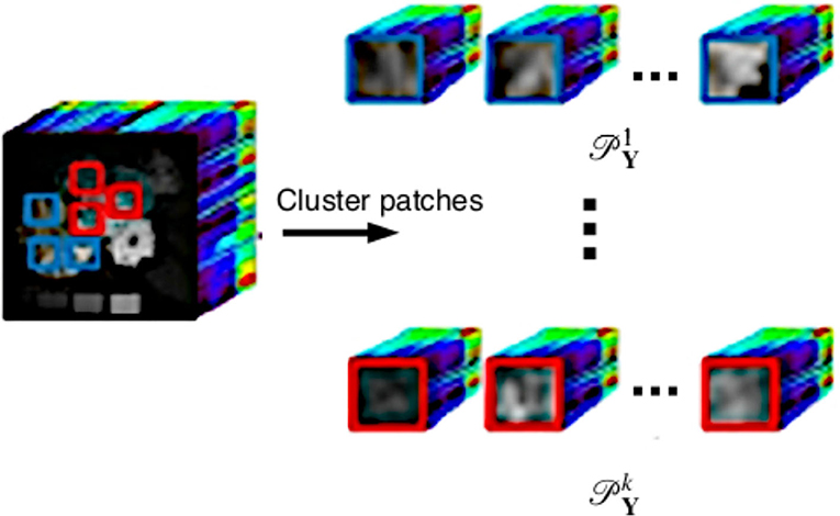
Figure 2. Clustering the set of patches ${{P}}_Y$ into k = 2 classes.

Following the clustering, we consider each set of patches ${{P}}_Y^i={\{Y_{p_j}\}}_{j\in I_i}$, for some index set I_i with 1 ≤ i ≤ k. Let $Y_{(\lambda ,I_i)}\in {ℝ}^{m_p{m}_p\times \lambda N_{I_i}}$ and ${\hat{X}}_{(\lambda ,I_i)}\in {ℝ}^{n_p{n}_p\times \lambda N_{I_i}}$ represent the images corresponding to the set of LR and HR patches ${{P}}_Y^i$ and ${{P}}_{\hat{X}}^i$ defined by

$\begin{array}{ll}\begin{array}{c}{Y}_{(\lambda ,I_i)}=[y_{1,p_1},\dots ,y_{\lambda ,p_1},\dots ,y_{1,p_{N_{I_i}}},\dots ,y_{\lambda ,p_{N_{I_i}}}]\\ {\hat{X}}_{(\lambda ,I_i)}=[{\hat{x}}_{1,p_1},\dots ,{\hat{x}}_{\lambda ,p_1},\dots ,{\hat{x}}_{1,p_{N_{I_i}}},\dots ,{\hat{x}}_{\lambda ,p_{N_{I_i}}}]\end{array}& (24)\end{array}$

where n_p = ωm_p for some scale factor ω ∈ ℕ, y_i,pj and ${\hat{x}}_{i,p_j}$ represents the vectorization of the i-th band of the j-th patch, with 1 ≤ i ≤ λ and j ∈ I_i. Here, N_Ii represents the total number of patches in the set ${{P}}_Y^i$. Using the RKHS and AHF functions as in Deng et al. [40] we can find an embedding for the high-dimensional data that is also structure preserving. We further assume that the HR and LR image patches have similar local geometry and are related by the equations

$\begin{array}{ll}\begin{array}{c}{Y}_{(\lambda ,I_i)}=T^{\ell }D+K^{\ell }C+{\text{Ψ}}^{\ell }E,\\ {\hat{X}}_{(\lambda ,I_i)}=T^{h}D+K^{h}C+{\text{Ψ}}^{h}E,\end{array}& (25)\end{array}$

where $D=[d_1,\dots d_{\lambda N_{I_i}}]\in {ℝ}^{M\times \lambda N_{I_i}},C=[c_1,\dots c_{\lambda N_{I_i}}]\in {ℝ}^{m_1{m}_2\times \lambda N_{I_i}}$ and $E=[e_1,\dots e_{\lambda N_{I_i}}]\in {ℝ}^{n_{\theta }\times \lambda N_{I_i}}$ are coefficient matrices to be determined. The matrices T, K and Ψ represent the evaluations of the smooth, residual and edge components of the image intensity function on discrete grids. The superscript ℓ and h denote the coarse and fine grids and correspond to lower and higher resolution, respectively. We obtain the fine and coarse scale matrices T and K following the discretization models outlined in section 2.1 Similarly, we follow the discretization in section 2.2 to generate Ψ^ℓ and Ψ^h. The coefficient matrices are obtained by solving the following minimization problem for each patch indexed by i:

$\begin{array}{l}\underset{D,C,E}{\text{min}}\{\frac{1}{2}\Vert T^{\ell }D+K^{\ell }C+{\Psi }^{\ell }E-Y_{(\lambda ,I_i)}{\Vert }_F^2\\ +\frac{{\mu }_1}{2}{\displaystyle \sum _{jk}{w}_{jk}}\Vert d_j-d_k{\Vert }_2^2+\frac{{\mu }_2}{2}\text{tr}\left(C^T{K}^{\ell }C\right)+{\mu }_3\Vert E{\Vert }_{1,1}\}& (26)\end{array}$

with tr(·) as the trace and adaptive weights

$\begin{array}{ll}{w}_{jk}=\text{exp}\left(-\frac{\Vert d_j-d_k\Vert { }_2^2}{\sigma }\right),\sigma >0,& (27)\end{array}$

where D = [d₁, …d_λNIi] and μ₁, μ₂, μ₃ ≥ 0. Note that $\text{exp}\left(-\frac{\Vert d_j-d_k{\Vert }_2^2}{\sigma }\right)\Vert d_j-d_k{\Vert }_2^2$ is a unimodal function of $\Vert d_j-d_k{\Vert }_2^2$ that is maximized at 1 and minimized at zero and ∞. To simplify the computations, the adaptive weights are computed using the coefficients from a previous iteration. The first term of (26) is the data fidelity. There are three regularization terms in our proposed model. We assume that coefficients d_i are likely to vary smoothly within the same class of images. When d_i and d_j fall into the same class, w_ij tends to be larger, forcing the next iterate of d_i and d_j to be close as well. The second regularization term is a structure guided regularity following from (16) to guarantee that the coefficients of the residual components do not grow too large. Finally, we impose sparsity constraints using the ||·||_{1, 1} norm [48] defined by

$\begin{array}{ll}\Vert A{\Vert }_{1,1}={\displaystyle \sum _s^S}\Vert a_s{\Vert }_1,A=\left[a_1,\dots ,a_S\right],& (28)\end{array}$

since we assume that edges are sparse in the image patches. The resulting minimization can be solved using splitting techniques to obtain closed form solutions for the coefficients. We solve (26) iteratively using the alternating direction method of multipliers (ADMM) algorithm [49, 50].

Due to the non-differentiability of the ||·||_{1, 1} norm, we introduce a new variable U and solve the equality-constrained optimization problem

$\begin{array}{l}\underset{D,C,E,U}{\text{min}}\{\frac{1}{2}\Vert T^{\ell }D+K^{\ell }C+{\Psi }^{\ell }E-Y_{(\lambda ,I_i)}{\Vert }_F^2\\ +\frac{{\mu }_1}{2}{\displaystyle \sum _{jk}{w}_{jk}}\Vert d_j-d_k{\Vert }_2^2+\frac{{\mu }_2}{2}\text{tr}\left(C^T{K}^{\ell }C\right)+{\mu }_3\Vert U{\Vert }_{1,1}\}\\ \text{subject to }U=E.& (29)\end{array}$

By introducing the augmented Lagrangian and completing the squares, we change the constrained optimization problem (29) into the following non-constrained optimization where V is Lagrangian multiplier,

$\begin{array}{l}\underset{D,C,E,U}{\text{min}}\{\frac{1}{2}\Vert T^{\ell }D+K^{\ell }C+{\Psi }^{\ell }E-Y_{(\lambda ,I_i)}{\Vert }_F^2\\ +\frac{{\mu }_1}{2}{\displaystyle \sum _{jk}{w}_{jk}}\Vert d_j-d_k{\Vert }_2^2+\frac{{\mu }_2}{2}\text{tr}\left(C^T{K}^{\ell }C\right)\\ +{\mu }_3\Vert U{\Vert }_{1,1}+\frac{\gamma }{2}\Vert U-E+\frac{V}{\gamma }{\Vert }_F^2\}& (30)\end{array}$

with step length γ ≥ 0. ADMM reduces (30) to solving the following separable subproblems:

• D subproblem:

$\begin{array}{l}\underset{D}{\text{min}}\{\frac{1}{2}\Vert T^{\ell }D+K^{\ell }C+{\Psi }^{\ell }E-Y_{(\lambda ,I_i)}{\Vert }_F^2\\ +\frac{{\mu }_1}{2}{\displaystyle \sum _{jk}{w}_{jk}}\Vert d_j-d_k{\Vert }_2^2\}.\end{array}$

Given that D = [d₁, …d_λNIi], C = [c₁, …c_λNIi], E = [e₁, …e_λNIi] and we can solve for each column of D separately

$\underset{d_j}{\text{min}}\{\frac{1}{2}\Vert T^{\ell }{d}_j+K^{\ell }{c}_j+{\Psi }^{\ell }{e}_j-y{\Vert }_F^2+\frac{{\mu }_1}{2}{\displaystyle \sum _{jk}{w}_{jk}}\Vert d_j-d_k{\Vert }_2^2\},$

where y is the corresponding column in Y_(λ,Ii) matching the column index of d_j. This gives a solution

$\begin{array}{l}{d}_j={\left(T^{\ell T}{T}^{\ell }+{\mu }_1{\displaystyle \sum _{jk}{w}_{jk}}I\right)}^{-1}(T^{\ell T}{T}^{\ell }y-T^{\ell T}{K}^{\ell }{c}_j\\ -T^{\ell T}{\Psi }^{\ell }{e}_j+{\mu }_1{\displaystyle \sum _{jk}{w}_{jk}}{d}_k).\end{array}$

where $T^{{\ell }_T}$ represents the transpose of T^ℓ.

• C subproblem:

$\underset{c}{\text{min}}\left\{\frac{1}{2}\Vert T^{\ell }D+K^{\ell }C+{\Psi }^{\ell }E-Y_{(\lambda ,I_i)}{\Vert }_F^2+\frac{{\mu }_2}{2}\text{tr}\left(C^T{K}^{\ell }C\right)\right\}.$

From which we get

$\begin{array}{l}C={\left(K^{\ell T}{K}^{\ell }+{\mu }_2{K}^{\ell }\right)}^{-1}(K^{\ell T}{Y}_{(\lambda ,I_i)}\\ -K^{\ell T}{T}^{\ell }D-K^{\ell T}{\Psi }^{\ell }E).\end{array}$

• E subproblem:

$\underset{E}{\text{min}}\left\{\frac{1}{2}\Vert T^{\ell }D+K^{\ell }C+{\Psi }^{\ell }E-Y_{(\lambda ,I_i)}{\Vert }_F^2+\frac{\gamma }{2}\Vert U-E+\frac{V}{\gamma }{\Vert }_F^2\right\}.$

Similarly, this gives the solution

$\begin{array}{l}E={\left({\Psi }^{\ell T}{\Psi }^{\ell }+\gamma 1I\right)}^{-1}({\Psi }^{\ell T}{Y}_{(\lambda ,I_i)}-{\Psi }^{\ell T}{T}^{\ell }D\\ -{\Psi }^{\ell T}{K}^{\ell }C+\gamma \left(U+V\right)).\end{array}$

• U subproblem:

$\underset{U}{\text{min}}\left\{{\mu }_3\Vert U{\Vert }_{1,1}+\frac{\gamma }{2}\Vert U-E+\frac{V}{\gamma }{\Vert }_F^2\right\}.$

A solution to this problem arising from the group sparsity constraint can be obtained by applying ℓ₁ shrinkage to the rows of U, i.e.,

$\begin{array}{l}{u}_j^T=\text{shrink }(u_j^T+v_j^T/\gamma ,{\mu }_3/\gamma ),\end{array}$

where

$\text{shrink}(x,\gamma )=\{\begin{array}{ll}{x}_i-\nu ,\hfill & \text{if }{x}_i>\gamma ,\hfill \\ x_i+\nu ,\hfill & \text{if }{x}_i<-\gamma ,\hfill \\ 0,\hfill & \text{otherwise}\hfill \end{array}$

for any x ∈ ℝⁿ and γ > 0.

The update for V is obtained by

$\begin{array}{l}V=V+\gamma (E-U).\end{array}$

The estimated set of patches ${{P}}_{\hat{X}}$ can be generated using (25) once the coefficients have been obtained. After running through the procedure for all the k sets, we consolidate the patches to form the enhanced resolution result $\hat{X}$. The proposed algorithm for SISR is summarized in Algorithm 1. Step 3 contains most of the key components of the algorithm so we provide more details. An outer layer loop is used to pick up residuals and put them back into the super resolution algorithm to further enhance the results. τ is the total number of outer layer iterations, B and S are the blurring and downsampling matrices, respectively. In the absence of blur, B becomes the identity matrix. Starting from one cluster of low resolution image patches, Step 3(b) solves the minimization problem (30) to obtain the coefficients C, D, E, from which one is able to assemble a higher resolution image as shown in Step 3(c). From this higher resolution image, we can create a lower resolution image by applying SB operator on it. Step 3(d) calculates the error between the actual low resolution and the simulated one. If the higher resolution image is close to the ground truth, we expect the error to be small. Otherwise, we feeding this difference into the minimization problem (30) can further recover more details. These details are added to the previously recovered higher resolution image to achieve a better image [40].

ALGORITHM 1

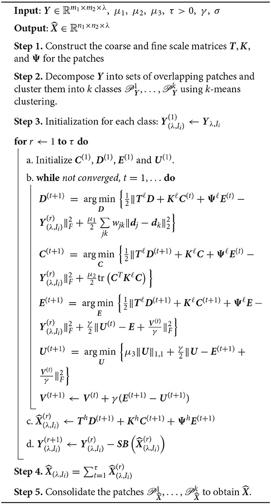
Algorithm 1: Analog three-dimensional single image SR model.

3.2. Pansharpening

Given a LR MS image Y and a high spatial resolution PAN image (P) matching the same scene, our goal is to estimate a HR MS image $\hat{X}$ with the spatial dimensions of the PAN. We propose a two-stage approach to solve the pansharpening problem. To begin with, we obtain a preliminary estimate for the target image $\tilde{Y}$ using CS or MRA, two fast and simple pansharpening techniques. $\tilde{Y}$ has the same size as $\hat{X}$ but the result $\tilde{Y}$ obtained using these methods suffer from spectral and spatial distortion drawbacks. The second step in our proposed two-stage approach provides a way to reduce the drawbacks. Next, we feed Algorithm 1 with input $\tilde{Y}$ and proceed with the resulting optimization model to generate $\hat{X}$. Considering the image $\tilde{Y}$, the modified optimization model becomes

$\begin{array}{l}\underset{D,C,E}{\text{min}}\{\frac{1}{2}\Vert T^{h}D+K^{h}C+{\Psi }^{h}E-{\tilde{Y}}_{(\lambda ,I_i)}{\Vert }_F^2\\ +\frac{{\mu }_1}{2}{\displaystyle \sum }_{jk}{w}_{jk}\Vert d_j-d_k{\Vert }_2^2\frac{{\mu }_2}{2}\text{tr}\left(C^T{K}^{\ell }C\right)+{\mu }_3\Vert E{\Vert }_{1,1}\},& (31)\end{array}$

where ${\tilde{Y}}_{(\lambda ,I_i)}=[{\tilde{y}}_{1,p_1},\dots ,{\tilde{y}}_{\lambda ,p_1},\dots ,{\tilde{y}}_{1,p_{N_{I_i}}},\dots ,{\tilde{y}}_{\lambda ,p_{N_{I_i}}}]\in {ℝ}^{n_p{n}_p\times \lambda N_{I_i}}$ for the set of patches ${{P}}_{\tilde{Y}}^i$, 1 ≤ i ≤ k. K-means clustering is used to decompose the number of overlapping patches into k classes, so that pixels corresponding to similar kinds of objects in the image will be collectively estimated in each step. The optimal value of k for a given image was determined using the silhouette method [51] which measures how similar a point is to its own cluster compared to other clusters. The adaptive weights are defined the same way as in (27). Applying ADMM to (31) we can solve the separable subproblems that ensue for the coefficients D, C and E as in the single image model. We summarize the procedure in Algorithm 2.

ALGORITHM 2

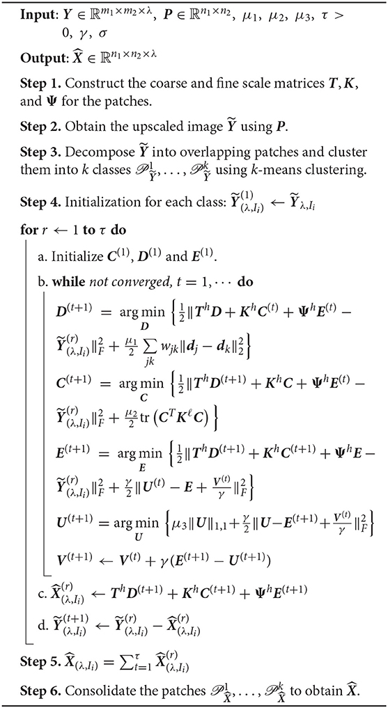
Algorithm 2: Pansharpening model

4. Experimental Results

4.1. Simulation Protocol

To begin with the simulation procedure, we test the performance of the proposed algorithm by generating the reduced resolution image from a given image for some chosen downscaling factors. We then compute the enhanced resolution result using the proposed algorithm and compare its performance with other methods. The experiments are implemented using MATLAB(R2018a).

For the SISR experiments we compare our three-dimensional single image super-resolution algorithm to bicubic interpolation and the RKHS algorithm by Deng et al. [40]. The authors in Deng et al. [40] implement their SR algorithm following an independent band procedure. For color images (RGB), they transform the image to the “YCbCr” color space and apply model in Deng et al. [40] to the luma component (Y) only since humans are more sensitive to luminance changes. The “Cb” and “Cr” components are the blue-difference and the red-difference chroma components, respectively. This way, the time complexity of the algorithm is reduced, as compared to an optimization based methods using all the channels at the same time. To obtain the desired result, the chroma components (Cb, Cr) are upscaled by bicubic interpolation. The components are then transformed back to the RGB color space for further analysis. In our approach, we apply Algorithm 1 to the three-dimensional color images directly, without undertaking any transformations.

We undertake the pansharpening experiments using semi-synthetic test data. This may be attributed to the fact that existing sensors cannot readily provide images at the increased spatial resolution that is desired. A generally acceptable procedure attributed to Ranchin and Wald [23] for operating at reduced resolution is as follows (Illustration in Figure 3):

• The enhanced result should be as identical as possible to the original multispectral image once it has been degraded.

• The enhanced result should be identical to the corresponding high resolution image that a capable sensor would observe at the increased resolution.

• Each band of the enhance result should be as identical as possible to the corresponding bands of the image that would have been observed by a sensor with high resolution.

FIGURE 3

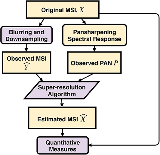
Figure 3. Flow diagram of the experimental procedure for synthetic datasets.

We apply Algorithm 2 to the observed multispectral data and compare it with existing state-of-the-art approaches.

4.2. Parameter Selection

Parameter selection is essential to obtain good results. However, to show the stability of our proposed method, we fix the parameters for all the experiments. Fine tuning of the parameters might lead to slightly better results. Parameter choices for the optimization of our proposed algorithms are outlined as follows:

• Scale factor (ω): In the experiments shown above, we set ω = 2 for the SISR problem, and set ω = 4 for the pansharpening problem. Quantitative measures obtained suggest that for ω > 4 both problems yield unsatisfactory results as the spatial and spectral measures are less competitive. However, the choice of ω depends on the dimensions of the observed data. For large ω, we can select larger patch sizes to improve upon the target.

• Patch size (m_p): Patch sizes can vary according to the size of the given image. We use a default patch size, m_p × m_p × λ in our experiments. Reasonable quantitative measures were obtained for 6 ≤ m_p ≤ 8 for the two problems considered. Outside the given bounds, the algorithms either take time to converge or yield unsatisfactory results.

• Overlap size: The limits of the overlapping region range from 2 to 4 are limited by the patch size. We set the overlap size to 2.

• Number of classes (k): In our experiments, the value of k was decided based on the solution that gave the best result from the silhouette method [51], i.e., by combing through predetermined values. Future work will involve investigating whether it is possible to automate this step.

• Construction of approximation matrices T, K, and Ψ: We generate the matrices based on the procedure outlined in section 3, with M = 6, ε = 1e⁻³, and set 20 evenly distributed angles on [0, 2π] in computing the fine and coarse scale matrices for T, K and Ψ, respectively.

• Regularization penalties μ₁, μ₂, μ₃ and γ: Without knowledge of optimal values for the penalty, we sweep through a range of values to determine the optimal result. For the experiments considered, μ₁, μ₂, μ₃, γ ∈ {10⁻⁸, ⋯ , 10²} and choose the one that leads to the best results evaluated by quantitative and qualitative measures. The step length γ for updating of V influences the convergence of the algorithm greatly.

• Preprocessing for Algorithm 2: Our proposed pansharpening method provides a flexible way to improve the results for both CS and MRA algorithms. In the experiments shown above, we preprocess the images using the GS algorithm. Future work will detail which preprocessing step works best for multispectral images.

4.3. Quantitative Criteria

To measure the similarity of the enhanced resolution image ($\hat{X}$) to the reference image (X), we compute the following image quality metrics:

• Correlation coefficient (CC): The correlation coefficient measures the similarity of spectral features between the reference and pansharpened image. It is defined as

$\begin{array}{l}\text{CC}(\hat{X})=\frac{1}{\lambda }{\displaystyle \sum _{i=1}^{\lambda }}\frac{1}{{\sigma }_{{\hat{X}}_i}{\sigma }_{X_i}}\text{E}[({\hat{X}}_i-{\mu }_{{\hat{X}}_i})(X_i-{\mu }_{X_i})]\end{array}$

where X_i and ${\hat{X}}_i$ are the matrices of the i-th band of X and $\hat{X}$, with μ_Xi and ${\mu }_{{\hat{X}}_i}$ as their respective mean gray values. The standard deviations for ${\hat{X}}_i$ and X_i are ${\sigma }_{{\hat{X}}_i}$ and σ_Xi, respectively.

• Root mean square error (RMSE):

$\begin{array}{l}\text{RMSE}(\hat{X})=\sqrt{\text{MSE}(\hat{X})},\end{array}$

where

$\text{MSE}(\hat{X})=E[{(\hat{X}-X)}^2]=\frac{\Vert \hat{X}-X\Vert {}_F^2}{n_1{n}_2\lambda }$

• Peak signal-to-noise ratio (PSNR): It is an expression of the ratio between the maximum possible value of the signal and the distorting noise that affects the quality of the representation.

$\begin{array}{l}\text{PSNR}(\hat{X})=20·{\text{log}}_{10}\left(\frac{{\text{MAX}}_{\hat{X}}}{\sqrt{\text{MSE}(\hat{X})}}\right)\end{array}$

• Structural Similarity (SSIM): The SSIM index is computed by examining various windows of the reference and target image. It is a full reference metric designed to improve upon the traditional methods such as PNSR and MSE.

• Spectral angle mapper (SAM): This measure denotes the absolute value of the angle between the reference and estimated spectral vectors.

Let ${\hat{X}}_{\left\{i\right\}}={({\widehat{x}}_{i,1},\dots ,{\widehat{x}}_{i,\lambda })}^T,1\le i\le n_1{n}_2$ be a vector collecting the intensity at all spectral bands at pixel i,

$\begin{array}{l}\text{SAM}(\hat{X})=\frac{1}{n_1{n}_2}{\displaystyle \sum _{i=1}^{n_1{n}_2}}\text{arcos}\left(\frac{\langle {\hat{X}}_{\left\{i\right\}},X_{\left\{i\right\}}\rangle }{\Vert {\hat{X}}_{\left\{i\right\}}\Vert \Vert X_{\left\{i\right\}}\Vert }\right)\end{array}$

• Erreur relative globale adimensionnelle de synthése (ERGAS): The relative dimensionless global error in the synthesis reflects the overall quality of the pansharpened image.

$\begin{array}{l}\text{ERGAS}(\hat{X})=100d\sqrt{\frac{1}{\lambda }{\displaystyle \sum _{i=1}^{\lambda }}{\left(\frac{\text{RMSE}({\hat{X}}_i)}{{\mu }_{{\hat{X}}_i}}\right)}^2},\\ d=\text{downsampling factor}.\end{array}$

• Q index: It defines a universal measure that combines the loss of correlation, luminance, and contrast distortion of an image and is defined by

$Q(\widehat{X})=\frac{1}{\lambda }{\displaystyle \sum _{i=1}^{\lambda }\frac{4{\sigma }_{(X_i,{\widehat{X}}_i)}{\mu }_{X_i}{\mu }_{{\widehat{X}}_i}}{({\sigma }_{X_i}^2+{\sigma }_{{\widehat{X}}_i}^2)[{\mu }_{X_i}^2+{\mu }_{{\widehat{X}}_i}^2])}}$

where ${\sigma }_{(X_i,{\hat{X}}_i)}$ is the covariance between X_i and ${\hat{X}}_i$.

4.4. Results

In this section, we compare the visual results and quantitative measures of the proposed approaches with some existing super-resolution algorithms. The results of Algorithm 1 will be compared to bicubic interpolation and the RKHS model by Deng et al. [40]. Results of Algorithm 2 are compared with CS methods such as PCA, IHS, Brovey, GS and Indusion, as well as MRA methods such as HPF, SFIM, ATWT, AWLP, GLP techniques, and the Deng et al. pansharpening model [43]. We begin with numerical tests for true color images and consider patches of size 8 × 8 × λ. The size of the overlap across the vertical and horizontal dimensions is 2.

In Figure 4, we show one example of decomposing an original image into three components. One can see that the edge information is separated successfully from the smooth component and the residual. In Figure 5, we compare 3D super resolution result of the proposed model with bicubic interpolation and RKHS [40] on a baboon image. We can see that the proposed method leads to a color image with highest visual quality. The bicubic interpolation result tends to be blurry. RKHS [40] result is better but not as good as the proposed. In Table 1, we list some quantitative metric comparison for more testing images. It is observed that the proposed 3D single image super resolution method (detailed in Algorithm 1) is consistently the best among the three approaches.

FIGURE 4

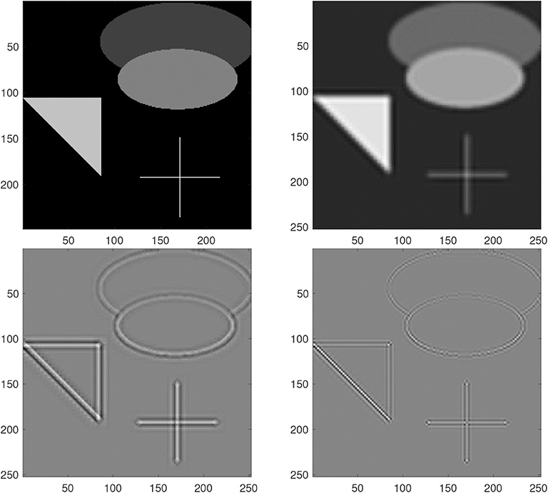
Figure 4. Decomposition of components for the grayscale test image. From top to bottom and left to right: the original, T^hD, K^hC, Ψ^hE.

FIGURE 5

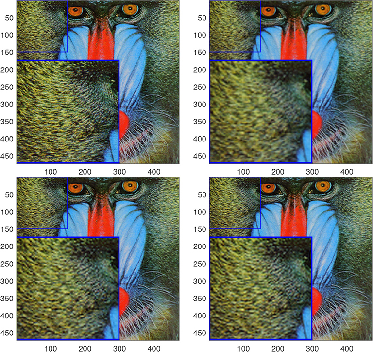
Figure 5. Results for baboon using a scale factor ω = 2. From top to bottom and left to right: ground truth, bicubic interpolation, RKHS [40] and the proposed.

TABLE 1

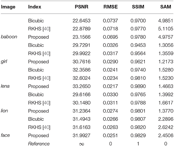
Table 1. Quantitative Results with for single image super-resolution with ω = 2.

For pansharpening, we compare with 10 other methods in the literature using five different quantitative metrics (see Table 2). It is observed that the proposed pansharpening method (detailed in Algorithm 2) is mostly the best and occasionally the second among all. The performance is consistently superior.

TABLE 2

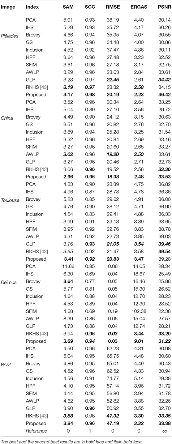
Table 2. Quantitative Results with for pansharpening ω = 4

Note that we did not conduct comparison with deep neural network based methods. The proposed approach is based on single image modeling while the deep neural network approach relies on a lot of external data. We don't think it is a fair comparison.

5. Conclusions

In this paper, we have proposed a technique for single image SR by modeling the image as a linear combination of regular functions in tandem with sparse coding. We show that the proposed scheme is an improvement upon similar existing approaches as it outperforms these algorithms. Besides this advantage, the proposed methods can also benefit image decomposition.

In future work, we will apply the model to multispectral and hyperspectral image SR where sparse coding can be useful due to the redundant nature of the input.

Data Availability Statement

Some of the datasets for this study can be found in http://openremotesensing.net.

Author Contributions

WG contributes on providing the main ideas including the mathematical models and algorithms proposed in the paper. RL was a former Ph.D. student of WG. Under WG's guidance, RL did computer programming to implement the ideas and conducted numerical experiments to test the effective of the proposed method compared to the state of the art. XZ and CG are domain scientists who help us evaluate the numerical results and provide comments.

Funding

WG was supported by National Science Foundation (DMS-1521582).

Conflict of Interest

The authors declare that the research was conducted in the absence of any commercial or financial relationships that could be construed as a potential conflict of interest.

References

1. Farsiu S, Robinson D, Elad M, Milanfar P. Advances and challenges in super-resolution. Int J Imaging Syst Technol. (2004) 14:47–57. doi: 10.1002/ima.20007

CrossRef Full Text | Google Scholar

2. Yang C-Y, Ma C, Yang M-H. Single-image super-resolution: a benchmark. In: European Conference on Computer Vision. Cham: Springer (2014). p. 372–86. doi: 10.1007/978-3-319-10593-2_25

PubMed Abstract | CrossRef Full Text | Google Scholar

3. Park SC, Park MK, Kang MG. Super-resolution image reconstruction: a technical overview. IEEE Signal Process Mag. (2003) 20:21–36. doi: 10.1109/MSP.2003.1203207

CrossRef Full Text | Google Scholar

4. Baker S, Kanade T. Limits on super-resolution and how to break them. IEEE Trans Pattern Anal Mach Intell. (2002) 24:1167–83. doi: 10.1109/TPAMI.2002.1033210

CrossRef Full Text | Google Scholar

5. Lin Z, Shum H-Y. Fundamental limits of reconstruction-based superresolution algorithms under local translation. IEEE Trans Pattern Anal Mach Intell. (2004) 26:83–97. doi: 10.1109/TPAMI.2004.1261081

PubMed Abstract | CrossRef Full Text | Google Scholar

6. Thévenaz P, Blu T, Unser M. Interpolation revisited [medical images application]. IEEE Trans Pattern Anal Mach Intell. (2000) 19:739–758. doi: 10.1109/42.875199

PubMed Abstract | CrossRef Full Text | Google Scholar

7. Keys R. Cubic convolution interpolation for digital image processing. IEEE Trans Acoust Speech Signal Process. (1981) 29:1153–60. doi: 10.1109/TASSP.1981.1163711

CrossRef Full Text | Google Scholar

8. Glasner D, Bagon S, Irani M. Super-resolution from a single image. In: IEEE 12th International Conference on Computer Vision, 2009. IEEE (2009). p. 349–56. doi: 10.1109/ICCV.2009.5459271

CrossRef Full Text | Google Scholar

9. Freedman G, Fattal R. Image and video upscaling from local selfexamples. ACM Trans Graph. (2011) 30:12. doi: 10.1145/2010324.1964943

CrossRef Full Text | Google Scholar

10. Gao X, Zhang K, Tao D, Li X. Joint learning for single-image super-resolution via a coupled constraint. IEEE Trans Image Process. (2012) 21:469–80. doi: 10.1109/TIP.2011.2161482

PubMed Abstract | CrossRef Full Text | Google Scholar

11. Wang Z, Yang Y, Wang Z, Chang S, Yang J, Huang TS. Learning super-resolution jointly from external and internal examples. IEEE Trans Image Process. (2015) 24:4359–71. doi: 10.1109/TIP.2015.2462113

PubMed Abstract | CrossRef Full Text | Google Scholar

12. Yang J, Wright J, Huang TS, Ma Y. Image super-resolution via sparse representation. IEEE Trans Image Process. (2010) 19:2861–73. doi: 10.1109/TIP.2010.2050625

PubMed Abstract | CrossRef Full Text | Google Scholar

13. Bioucas-Dias JM, Figueiredo MA. A new twist: two-step iterative shrinkage/thresholding algorithms for image restoration. IEEE Trans Image Process. (2007) 16:2992–3004. doi: 10.1109/TIP.2007.909319

PubMed Abstract | CrossRef Full Text | Google Scholar

14. Rudin LI, Osher S. Total variation based image restoration with free local constraints. In: IEEE International Conference on Image Processing, 1994. ICIP-94. IEEE (1994). p. 31–5.

Google Scholar

15. Getreuer P. Contour stencils: Total variation along curves for adaptive image interpolation. SIAM J Imaging Sci. (2011) 4:954–79. doi: 10.1137/100802785

CrossRef Full Text | Google Scholar

16. Kim KI, Kwon Y. Single-image super-resolution using sparse regression and natural image prior. IEEE Trans Pattern Anal Mach Intell. (2010) 32:1127–33. doi: 10.1109/TPAMI.2010.25

PubMed Abstract | CrossRef Full Text | Google Scholar

17. Sun J, Xu Z, Shum H-Y. Image super-resolution using gradient profile prior. In: IEEE Conference on Computer Vision and Pattern Recognition, 2008. CVPR. IEEE (2008). p. 1–8.

PubMed Abstract | Google Scholar

18. Fattal R. Image upsampling via imposed edge statistics. ACM Trans Graph. (2007) 26:95. doi: 10.1145/1276377.1276496

CrossRef Full Text | Google Scholar

19. Lium B, Son S, Kim H, Nah S, Mu K. Enhanced deep residual networks for single image super-resolution. In: The IEEE Conference on Computer Vision and Pattern Recognition (CVPR) Workshops. (2017).

Google Scholar

20. Yang W, Zhang X, Tian Y, Wang W, Xue J, Liao Q. Deep learning for single image super-resolution: a brief review. IEEE Trans Multimedia. (2019) 21:3106–21. doi: 10.1109/TMM.2019.2919431

CrossRef Full Text | Google Scholar

21. Wang Y, Wang L, Wang H, Li P. End-to-end image super-resolution via deep and shallow convolutional networks. IEEE Access. (2019) 7:31959–70. doi: 10.1109/ACCESS.2019.2903582

CrossRef Full Text | Google Scholar

22. Li Z, Yang J, Liu Z, Yang X, Jeon G, Wu W. Feedback network for image super-resolution. In: IEEE Conference on Computer Vision and Pattern Recognition CVPR. Long Beach, CA: IEEE (2019). doi: 10.1109/CVPR.2019.00399

PubMed Abstract | CrossRef Full Text | Google Scholar

23. Ranchin T, Wald L. Fusion of high spatial and spectral resolution images: the ARSIS concept and its implementation. Photogram Eng Remote Sens. (2000) 66:49–61.

Google Scholar

24. Loncan L, de Almeida LB, Bioucas-Dias JM, Briottet X, Chanussot J, Dobigeon N, et al. Hyperspectral pansharpening: a review. IEEE Geosci Remote Sens Mag. (2015) 3:27–46. doi: 10.1109/MGRS.2015.2440094

CrossRef Full Text | Google Scholar

25. Vivone G, Alparone L, Chanussot J, Dalla Mura M, Garzelli A, Licciardi GA, et al. A critical comparison among pansharpening algorithms. IEEE Trans Geosci Remote Sens. (2015) 53:2565–86. doi: 10.1109/TGRS.2014.2361734

CrossRef Full Text | Google Scholar

26. Shettigara V. A generalized component substitution technique for spatial enhancement of multispectral images using a higher resolution data set. Photogramm Eng Remote Sens. (1992) 58:561–7.

Google Scholar

27. Shah VP, Younan NH, King RL. An efficient pan-sharpening method via a combined adaptive PCA approach and contourlets. IEEE Trans Geosci Remote Sens. (2008) 46:1323–35. doi: 10.1109/TGRS.2008.916211

CrossRef Full Text | Google Scholar

28. Tu T-M, Su S-C, Shyu H-C, Huang PS. A new look at IHS-like image fusion methods. Inform Fusion. (2001) 2:177–86. doi: 10.1016/S1566-2535(01)00036-7

CrossRef Full Text | Google Scholar

29. Carper JW, Lillesand TM, Kiefer RW. The use of intensityhue- saturation transformations for merging spot panchromatic and multispectral image data. Photogramm Eng Remote Sens. (1990) 56:459–67.

Google Scholar

30. Chavez P, Sides SC, Anderson JA. Comparison of three different methods to merge multiresolution and multispectral data: landsat TM and SPOT panchromatic. Photogramm Eng Remote Sens. (1991) 57:295–303.

Google Scholar

31. Gillespie AR, Kahle AB, Walker RE. Color enhancement of highly correlated images. I. Decorrelation and HSI contrast stretches. Remote Sens Environ. (1986) 20:209–35. doi: 10.1016/0034-4257(86)90044-1

CrossRef Full Text | Google Scholar

32. Laben CA, Brower BV. Process for Enhancing the Spatial Resolution of Multispectral Imagery Using Pan-Sharpening. US Patent 6011875 (2000).

Google Scholar

33. Liu J Smoothing filter-based intensity modulation: a spectral preserve image fusion technique for improving spatial details. Int J Remote Sens. (2000) 21:3461–72. doi: 10.1080/014311600750037499

CrossRef Full Text | Google Scholar

34. Aiazzi B, Alparone L, Baronti S, Garzelli A, Selva M. An MTF-based spectral distortion minimizing model for pan-sharpening of very high resolution multispectral images of urban areas. In: 2nd GRSS/ISPRS Joint Workshop on Remote Sensing and Data Fusion over Urban Areas. IEEE (2003). p. 90–4.

Google Scholar

35. Aiazzi B, Alparone L, Baronti S, Garzelli A, Selva M. MTF-tailored multiscale fusion of high-resolution MS and pan imagery. Photogramm Eng Remote Sens. (2006) 72:591–6. doi: 10.14358/PERS.72.5.591

CrossRef Full Text | Google Scholar

36. Vivone G, Restaino R, Dalla Mura M, Licciardi G, Chanussot J. Contrast and error-based fusion schemes for multispectral image pansharpening. IEEE Geosci Remote Sens Lett. (2014) 11:930–4. doi: 10.1109/LGRS.2013.2281996

CrossRef Full Text | Google Scholar

37. Otazu X, González-Audícana M, Fors O, Núñez J. Introduction of sensor spectral response into image fusion methods. Application to wavelet-based methods. IEEE Trans Geosci Remote Sens. (2005) 43:2376–85. doi: 10.1109/TGRS.2005.856106

CrossRef Full Text | Google Scholar

38. Hou L, Zhang X. Pansharpening image fusion using cross-channel correlation: a framelet-based approach. J Math Imaging Vis. (2016) 55:36–49. doi: 10.1007/s10851-015-0612-x

CrossRef Full Text | Google Scholar

39. He X, Condat L, Bioucas-Dias JM, Chanussot J, Xia J. A new pansharpening method based on spatial and spectral sparsity priors. IEEE Trans Image Process. (2014) 23:4160–74. doi: 10.1109/TIP.2014.2333661

PubMed Abstract | CrossRef Full Text | Google Scholar

40. Deng L-J, Guo W, Huang T-Z. Single-image super-resolution via an iterative reproducing kernel hilbert space method. IEEE Trans Circ Syst Video Technol. (2016) 26:2001–14. doi: 10.1109/TCSVT.2015.2475895

PubMed Abstract | CrossRef Full Text | Google Scholar

41. Wahba G, Spline Models for Observational Data. Society for Industrial and Applied Mathematics. Philadelphia, PA: Siam (1990). doi: 10.1137/1.9781611970128

CrossRef Full Text | Google Scholar

42. Irani M, Peleg S. Super resolution from image sequences. In: 10th International Conference on Pattern Recognition. IEEE (1990). p. 115–20.

PubMed Abstract | Google Scholar

43. Deng L-J, Vivone G, Guo W, Dalla Mura M, Chanussot J. A variational pansharpening approach based on reproducible kernel hilbert 12 space and heaviside function. IEEE Trans Image Process. (2018). doi: 10.1109/ICIP.2017.8296338

PubMed Abstract | CrossRef Full Text | Google Scholar

44. Duchon J. Splines minimizing rotation-invariant semi-norms in Sobolev spaces. In: Constructive theory of Functions of Several Variables. Berlin: Springer (1977). p. 85–100. doi: 10.1007/BFb0086566

CrossRef Full Text | Google Scholar

45. Meinguet J. Multivariate interpolation at arbitrary points made simple. Z Angew Math Phys. (1979) 30:292–304. doi: 10.1007/BF01601941

CrossRef Full Text | Google Scholar

46. Kainen P, Kůrková V, Vogt A. Best approximation by linear combinations of characteristic functions of half-spaces. J Approx Theory. (2003) 122:151–9. doi: 10.1016/S0021-9045(03)00072-8

CrossRef Full Text | Google Scholar

47. Arthur D, Vassilvitskii S. k-means++: the advantages of careful seeding. In: Proceedings of the Eighteenth Annual ACM-SIAM Symposium on Discrete Algorithms. Society for Industrial and Applied Mathematics. (2007). p. 1027–35.

Google Scholar

48. Kowalski M. Sparse regression using mixed norms. Appl Comput Harm Anal. (2009) 27:303–24. doi: 10.1016/j.acha.2009.05.006

CrossRef Full Text | Google Scholar

49. Boyd S, Parikh N, Chu E, Peleato B, Eckstein J. Distributed optimization and statistical learning via the alternating direction method of multipliers. Found Trends Mach Learn. (2011) 3:1–122. doi: 10.1561/2200000016

CrossRef Full Text | Google Scholar

50. Eckstein J, Bertsekas DP. On the Douglas-Rachford splitting method and the proximal point algorithm for maximal monotone operators. Math Program. (1992) 55–3:293–318. doi: 10.1007/BF01581204

CrossRef Full Text | Google Scholar

51. Rousseeuw P. Silhouettes: a graphical aid to the interpretation and validation of cluster analysis. J Comput Appl Math. (1987) 20:53–65. doi: 10.1016/0377-0427(87)90125-7

CrossRef Full Text | Google Scholar