Complexity and Chimera States in a Ring-Coupled Fractional-Order Memristor Neural Network

1. Introduction

Forming networks is the nature of the world. There are many different examples of networks around us, such as social networks, electric power grids, the Internet, highways or subway systems, and neural networks [1–3]. Among these, a network of non-linear systems is an independent research branch and has become more and more important in the non-linear research field. Especially, the spatiotemporal behaviors of chaotic systems have been found to be interesting, and there are also many real applications based on these novel chaotic systems [4, 5]. Meanwhile, since neural systems can also be chaotic, spatiotemporal behaviors in the neural network have aroused much research interest [6]. The chimera state means that there is coexistence of synchronization and asynchronization in the network. There are many biological phenomena that can be explained by chimera states, such as unihemispheric sleep and brain disorders. For chimera states in a network of non-linear systems, Sajad's group has done a lot of remarkable work [7–10]. Meanwhile, the chimera states in different integer-order networks have been investigated, such as bursting neurons [11], ephaptically coupled bursting neurons [12], memristive neuron networks [13, 14], and three-dimensional locally coupled systems [15]. Moreover, there have also been many other studies on this topic [16–18].

Since the fractional-order calculus currently provides a more accurate mathematical tool for physical modeling, it has been widely used in many different research fields, such as non-uniform diffusion [19], boundary effects [20], and elastic deformation [21]. By introducing the fractional-order calculus to the network, the fractional-order network is designed. There are many different methods for connecting non-linear systems to build a fractional-order network. For instance, Chen et al. [22] analyzed the cluster synchronization of complex dynamical networks with fractional-order dynamical nodes by employing the stability theory of fractional-order differential systems. As a result, fractional-order complex networks with non-linear systems have been investigated theoretically [23, 24]. However, coupled control is the most direct way to build a network [25–27]. Because there are few references regarding numerical analysis of a fractional-order network, especially when chimera states exist, it is interesting to investigate chimera states in the coupled fractional-order network.

Complexity measurement provides an effective way to analyze the dynamics of chaotic systems by using the generated non-linear time series. Many different complexity analysis methods have been proposed, such as ApEn (approximate entropy) [28], SampEn (sample entropy) and FuzzyEn (fuzzy entropy) [29], SCM (statistical complexity measure) [30], the C₀ algorithm [31], and SE (spectral entropy) [32]. These methods estimate the complexity of non-linear time series from different angles. When a chaotic system has higher complexity, this means that the system can be chaotic; otherwise, the system is periodic or convergent. As a matter of fact, the results for complexity measure match well with those of the corresponding Lyapunov exponents analysis [33, 34]. For networks, there are also generated time series, but there are few articles on the complexity of networks. Thus, determining how to estimate the complexity of a network is an interesting topic.

The rest of this paper is organized as follows. In section 2, a fractional-order neural model and its dynamics are analyzed. In section 3, the formation and dynamics of the coupled neural network are investigated. Finally, section 4 summarizes the whole analysis.

2. The Fractional-Order Neural Model and Its Dynamics

2.1. The Neural Model

Ma and Tang [35] proposed an improved neural model by introducing additive variables describing magnet flux into the original HR neuron model based on the mean field theory. The neural model with memristor is defined by

$\begin{array}{ll}\{\begin{array}{c}\dot{x}=y-a{x}^3+b{x}^2-z+I_{ext}-k_{1}x\rho (w)\hfill \\ \dot{y}=c-d{x}^2-y\hfill \\ \dot{z}=r\left[s(x+1.6)-z\right]\hfill \\ \dot{w}=x-k_{2}w\hfill \end{array},\hfill & (1)\end{array}$

where x, y, z, and w are the system variables, and ρ(w) = α + βw² is the flux-controlled memristor. α and β are the fixed parameters, which are given by α = 0.1, β = 0.06. Meanwhile, the other parameters in the system are a = 1, b = 2.82, c = 1, d = 5, r = 0.02, s = 4, k₁ = −1, k₂ = 0.5, I_ext = 3.5.

By introducing the fractional calculus into the model, the fractional-order neural model is denoted as

$\begin{array}{ll}\{\begin{array}{c}{D}_{t_0}^{q}x=y-a{x}^3+b{x}^2-z+I_{ext}-k_{1}x\rho (w)\hfill \\ D_{t_0}^{q}y=c-d{x}^2-y\hfill \\ D_{t_0}^{q}z=r\left[s(x+1.6)-z\right]\hfill \\ D_{t_0}^{q}w=x-k_{2}w\hfill \end{array},\hfill & (2)\end{array}$

where q is the fractional derivative order. In this paper, $D_{t_0}^q$ is the Caputo fractional calculus, and its definition is given in Definition 1.

Definition 1 Gorenflo and Mainardi [36]: The Caputo fractional-order derivative definition is given by

$\begin{array}{ll}{D}_{t_0}^{q}x(t)=\{\begin{array}{c}\frac{1}{\Gamma (1-q)}{\int }_{t_0}^t\frac{\dot{x}(\tau )}{{(t-\tau )}^q}d\tau ,0<q<1\hfill \\ \dot{x}(t),q=1\hfill \end{array},\hfill & (3)\end{array}$

where q ∈ R⁺, m ∈ N, and Γ(·) is the Gamma function.

2.2. The Numerical Solution Algorithm

The Adam-Bashforth method (ABM) was proposed by Sun et al. [37], and it is widely used to solve fractional-order non-linear systems. Suppose that the fractional-order non-linear system is defined as

$\begin{array}{ll}\{\begin{array}{c}{D}_{t_0}^{q}x(t)=f(x,x(t)),0\le t\le T\hfill \\ x^{(k)}(0)=x_0^{(k)},k=0,1,2,\cdots ,\lceil q\rceil -1\hfill \end{array},\hfill & (4)\end{array}$

where $x^{(k)}(0)=x_0^{(k)}$ is the initial condition of the system, 0 < q ≤ 1, ⌈·⌉ is the ceil function and $D_{t_0}^{q}x(t)$ is the Caputo derivative.

According to Sun et al. [37], System (4) is equivalent to the Volterra integral equation

$\begin{array}{ll}x(t)={\displaystyle \sum _{k=0}^{\lceil q\rceil -1}}{x}_0^{(k)}\frac{t^k}{k!}+\frac{1}{\Gamma (q)}{\displaystyle {\int }_0^t}{(t-\tau )}^{q-1}f(\tau ,x(\tau ))d\tau ,\hfill & (5)\end{array}$

where

$\begin{array}{ll}{J}_t^{q}x(t)=\frac{1}{\Gamma (q)}{\displaystyle {\int }_0^t}{(t-\tau )}^{q-1}x(\tau )d(\tau ).\hfill & (6)\end{array}$

Let h = T/N, t_j = jh (j = 0, 1, ⋯, N ∈ Z⁺), the discrete solution of system (4) is

$\begin{array}{ll}\begin{array}{c}{x}_h(t_{n+1})={\displaystyle \sum _{k=0}^{\lceil q\rceil -1}}{x}_0^{(k)}\frac{t_{n+1}^k}{k!}+\frac{h^q}{\Gamma (q+2)}f(t_{n+1},x_h^p(t_{n+1}))\hfill \\ \hfill +\frac{h^q}{\Gamma (q+2)}{\displaystyle \sum _{j=0}^n}{\varphi }_{j,n+1}f(t_j,x_h(t_j))\hfill \end{array},\hfill & (7)\end{array}$

in which

$\begin{array}{ll}{x}_h^p(t_{n+1})={\displaystyle \sum _{k=0}^{\lceil q\rceil -1}}{x}_0^{(k)}\frac{t_{n+1}^k}{k!}+\frac{1}{\Gamma (q)}{\displaystyle \sum _{j=0}^n}{\phi }_{j,n+1}f(t_j,x_h(t_j)),\hfill & (8)\end{array}$

$\begin{array}{ll}{\phi }_{j,n+1}=\frac{h^q}{q}\left[{(n-j+1)}^q-{(n-j)}^q\right],0\le j\le n,\hfill & (9)\end{array}$

$\begin{array}{ll}{\varphi }_{j,n+1}=\{\begin{array}{c}{n}^{q+1}-(n-q){(n+1)}^q,j=0\hfill \\ {(n-j+2)}^{q+1}+{(n-j)}^{q+1}-2{(n-j+1)}^{q+1},1\le j\le n\hfill \\ 1,j=n+1\hfill \end{array}.\hfill & (10)\end{array}$

In this paper, the ABM algorithm is implemented in Matlab to solve the systems, and the function name is “FDE12.m”; this was developed by Roberto Garrappa.

2.3. Complex Dynamics

Fix a = 1, b = 2.82, c = 1, d = 5, r = 0.02, s = 4, k₁ = −1, k₂ = 0.5, and I_ext = 3.5, and let q = 0.7, q = 0.8, q = 0.9, and q = 1.0. The phase diagrams and time series of the system are illustrated in Figure 1. Here, when q = 1, the system is solved by the 4th-order Runge-Kutta method. It can be seen that the system is chaotic with the given parameters and derivative orders. Meanwhile, when the derivative order q takes smaller values, there is less fluctuation with time.

FIGURE 1

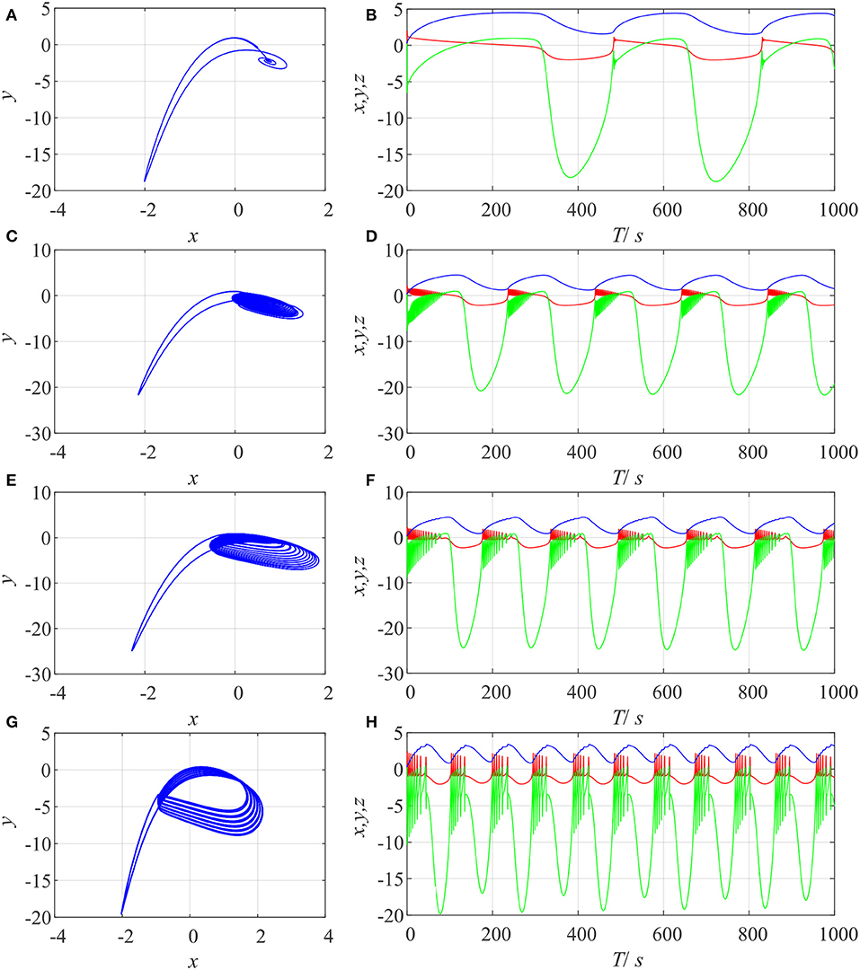
Figure 1. Phase diagrams and time series of the neural system with different values for derivative order q. (A) Phase diagram with q = 0.7; (B) time series with q = 0.7; (C) phase diagram with q = 0.8; (D) time series with q = 0.8; (E) phase diagram with q = 0.9; (F) time series with q = 0.9; (G) phase diagram with q = 1.0; (H) time series with q = 1.0.

When q = 1 and q = 0.99, the parameter I_ext varies from 3.5 to 4.5 with a step size of 0.002. When q = 0.9, I_ext varies from 0.5 to 5.5 with a step size of 0.01. The bifurcation diagrams and corresponding Lyapunov exponents (LEs) are shown in Figure 2. When q < 1, LEs are obtained by means of Danca and Kuznetsov [38], where the function [t, LE] = FO_Lyapunov(ne, ext_fcn, t_start, h_norm, t_end, x_start, h, q, out) is used. However, when q = 1, the LEs of the system are estimated by Wolf et al. [39]'s method, and the function [Texp, Lexp] = lyapunov(n, rhs_ext_fcn, fcn_integrator, tstart, stept, tend, ystart, ioutp) is employed. The function lyapunov.m can be download from the Mathworks website.

FIGURE 2

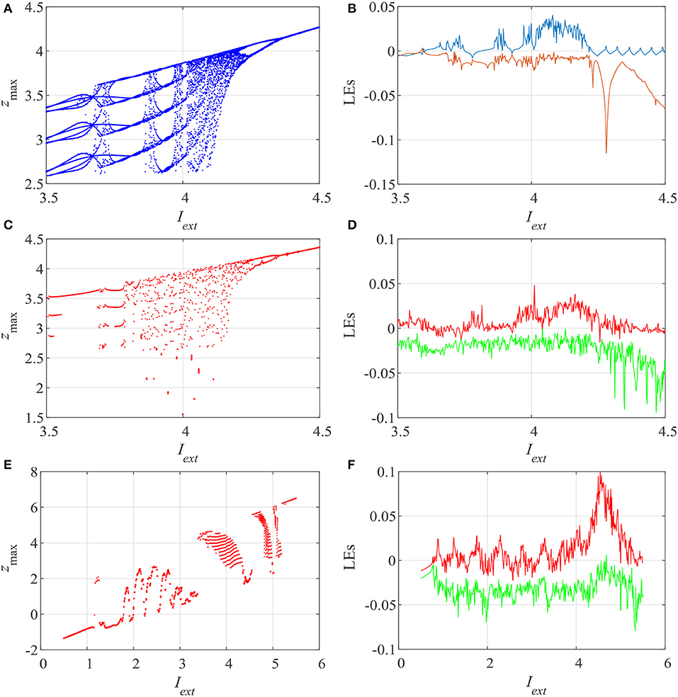
Figure 2. Results of analysis of the dynamics of the system with different values of derivative order q and variation in I_ext. (A) Bifurcation diagram with q = 1.0; (B) LEs with q = 1.0; (C) bifurcation diagram with q = 0.99; (D) LEs with q = 0.99; (E) bifurcation diagram with q = 0.9; (F) LEs with q = 0.9.

The plots in Figure 2 show that the system has rich dynamics with the variation of I_ext. Compared with the integer-order case, the fractional-order system has less periodic windows due to the memory effect of the fractional-order calculus. In fact, the Lyapunov exponents of the fractional-order chaotic system are calculated based on the short memory effect of the fractional-order calculus. Thus, the accuracy of the Lyapunov exponents is not as good as in the integer-order case. Overall, the bifurcation diagrams match well with corresponding the LEs, and the derivative order q has an influence on the system dynamics.

2.4. The Multiscale SE Algorithm

In this section, the spectral entropy (SE) algorithm is employed to analyze the complexity of the proposed SEIR system. For a one-dimensional discrete time series {x(n):n = 0, 1, ⋯ , N − 1}, the normalization entropy is estimated by Staniczenko et al. [32] and He et al. [40]

$\begin{array}{ll}SE(x^L)=\frac{1}{\text{ln }(N/2)}{\displaystyle \sum _{k=0}^{N/2-1}}{P}_k\text{ln }(P_k),\hfill & (11)\end{array}$

where ln(L/2) is the entropy of a completely random signal. The consecutive coarse-grained time series are constructed by Costa et al. [41]

$\begin{array}{ll}{y}^{\tau }(j)=\frac{1}{\tau }{\displaystyle \sum _{(j-1)\tau }^{j\tau -1}}x(j),\hfill & (12)\end{array}$

where 1 ≤ j ≤ [N/τ], τ is the scale factor, which represents the length of the non-overlapping window, and [·] denotes the floor function. As a result, the multiscale complexity is defined as [40]

$\begin{array}{ll}\text{MSE}=\frac{1}{{\tau }_{max}}{\displaystyle \sum _{\tau =1}^{{\tau }_{max}}}\text{SE}(y^{\tau }).\hfill & (13)\end{array}$

In this paper, we set τ_max = 25.

The variation of the complexity of the neural system with I_ext and different derivative order q values is investigated, and the results are shown in Figure 3. Figure 3 shows that the complexity of the system varies with parameter I_ext. When q = 1 and 0.91, the system has higher complexity, while when q = 0.9, the complexity of the system remains at a relatively low level, which means that the system has lower complexity when its derivative order is smaller than one. As shown in Figure 3, the results of the complexity analysis agree well with the corresponding Lyapunov exponents.

FIGURE 3

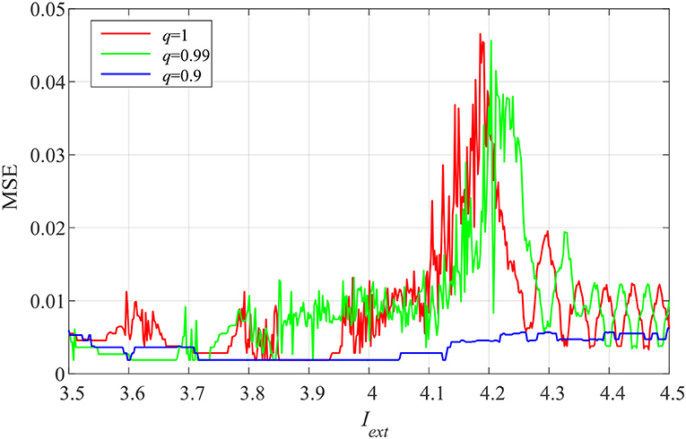
Figure 3. Analytical results for variation in the complexity of the system with I_ext for different values of derivative order q.

3. Formation and Dynamics of the Neural Network

3.1. Formation of the Network

The ring network of neural systems is investigated numerically. He et al. [26] investigated the synchronization of the ring network of a fractional-order simplified Lorenz chaotic system. The convergence of the network is investigated theoretically. In this paper, state variables of the chaotic systems in each node are coupled, and the numerical simulation results show the synchronization of the systems. In this paper, we consider different coupling methods: five different coupling methods are introduced.

The first case is where the coupling item is the variable, and it is defined as

$\begin{array}{ll}\{\begin{array}{c}{D}_{t_0}^q{x}_i=y_i-a{x}_i^3+b{x}_i^2-z+I_{ext}-k_1{x}_i\rho (w_i)\hfill \\ +\frac{D}{2}{\displaystyle \sum _{k=-1}^1}(x_k-x_i)\hfill \\ D_{t_0}^q{y}_i=c-d{x}_i^2-y_i\hfill \\ D_{t_0}^q{z}_i=r\left[s(x_i+1.6)-z_i\right]\hfill \\ D_{t_0}^q{w}_i=x_i-k_2{w}_i\hfill \end{array},\hfill & (14)\end{array}$

where D is the coupling strength.

The second method is to couple the system using the state variable y, and it is defined by

$\begin{array}{ll}\{\begin{array}{c}{D}_{t_0}^q{x}_i=y_i-a{x}_i^3+b{x}_i^2-z+I_{ext}-k_1{x}_i\rho (w_i)\hfill \\ D_{t_0}^q{y}_i=c-d{x}_i^2-y_i+\frac{D}{2}{\displaystyle \sum _{k=-1}^1}\left(y_k-y_i\right)\hfill \\ D_{t_0}^q{z}_i=r\left[s(x_i+1.6)-z_i\right]\hfill \\ D_{t_0}^q{w}_i=x_i-k_2{w}_i\hfill \end{array},\hfill & (15)\end{array}$

where $\frac{D}{2}{\displaystyle \sum _{k=-1}^1}(y_k-y_i)$ is the coupling item.

The third method is to couple the system using the state variable z, and it is defined by

$\begin{array}{ll}\{\begin{array}{c}{D}_{t_0}^q{x}_i=y_i-a{x}_i^3+b{x}_i^2-z+I_{ext}-k_1{x}_i\rho (w_i)\hfill \\ D_{t_0}^q{y}_i=c-d{x}_i^2-y_i\hfill \\ D_{t_0}^q{z}_i=r\left[s(x_i+1.6)-z_i\right]+\frac{D}{2}{\displaystyle \sum _{k=-1}^1}(z_k-z_i)\hfill \\ D_{t_0}^q{w}_i=x_i-k_2{w}_i\hfill \end{array}.\hfill & (16)\end{array}$

Here, D is the coupling strength. The other two cases (Case 4 and Case 5) are given by

$\begin{array}{ll}\{\begin{array}{c}{D}_{t_0}^q{x}_i=y_i-a{x}_i^3+b{x}_i^2-z+I_{ext}-k_1{x}_i\rho (w_i)\hfill \\ D_{t_0}^q{y}_i=c-d{x}_i^2-y_i\hfill \\ D_{t_0}^q{z}_i=r\left[s(x_i+1.6)-z_i\right]\hfill \\ D_{t_0}^q{w}_i=x_i-k_2{w}_i+\frac{D}{2}{\displaystyle \sum _{k=-1}^1}(w_k-w_i)\hfill \end{array},\hfill & (17)\end{array}$

and

$\begin{array}{ll}\{\begin{array}{c}{D}_{t_0}^q{x}_i=y_i-a{x}_i^3+b{x}_i^2-z+I_{ext}-k_1{x}_i\rho (w_i)\hfill \\ +\frac{D}{2}{\displaystyle \sum _{k=-1}^1}(x_k-x_i)\hfill \\ D_{t_0}^q{y}_i=c-d{x}_i^2-y_i+\frac{D}{2}{\displaystyle \sum _{k=-1}^1}\left(y_k-y_i\right)\hfill \\ D_{t_0}^q{z}_i=r\left[s(x_i+1.6)-z_i\right]+\frac{D}{2}{\displaystyle \sum _{k=-1}^1}(z_k-z_i)\hfill \\ D_{t_0}^q{w}_i=x_i-k_2{w}_i+\frac{D}{2}{\displaystyle \sum _{k=-1}^1}(w_k-w_i)\hfill \end{array}.\hfill & (18)\end{array}$

Obviously, in the fifth method, the systems are coupled with all the state variables.

The main difference between the five coupling methods is that the coupling variables are different. In the existing literature, scientists usually perform the coupling by all variables or just the first variable of the non-linear system in each node. In this paper, different coupling methods are considered, and how the coupling method affects the dynamics of the network is investigated.

3.2. Chimera State in the Network

The system parameters are a = 1, b = 2.82, c = 1, d = 5, r = 0.02, s = 4, k₁ = −1, k₂ = 0.5, I_ext = 3.5. The number of nodes is 100, and the initial conditions of the neural systems are set at a random number between 0 and 1.

Firstly, it should be noted that if the derivative order q = 1, the system is solved using the 4th-order Runge-Kutta method, while if q < 1, the network is solved by FDE12.m. The results of the numerical analysis of the five cases with different derivative order q values are illustrated in Figure 4, where the state variable x_i is used to draw the figures. Thus, these figures show the time evolution of the network. When the color is the same in the horizontal direction, it means that the output of each node of the network is the same, and synchronization exists in the network. Otherwise, asynchronization is observed in the network. Moreover, the chimera state means that both synchronization and asynchronization exist between different nodes over time. It can be seen clearly from Figure 4 that chimera states are observed in the network under different conditions. Generally speaking, when all of the state variables are coupled, the network synchronizes more easily. For instance, in Case 5, when q = 0.9, 0.8, and 0.7, the whole network is synchronized, but the chimera state is observed when q = 1. Meanwhile, compared with its integer-order counterpart, the fractional-order network is easier to synchronize. As shown in Figure 1, the dynamics of the neural system changes with the derivative order q. When the derivative order q decreases, the behaviors of the neural system become “simple." This is the main reason that the fractional-order network has less complexity.

FIGURE 4

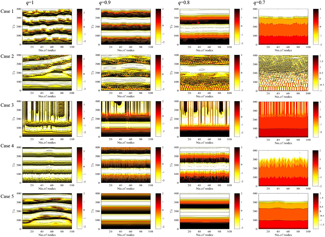
Figure 4. Results of numerical analysis of the neural network with different derivative order q values and different cases.

Whether the coupled network is chaotic or not depends on the state of the original neural system. If the original neural system is chaotic, the network is chaotic. Otherwise, the network is not chaotic. Take Case 5 as an example to show the dynamics of the network; the results are shown in Figure 5, where q = 1 and q = 0.9 for Figures 5A,B, respectively. The plots show that the x_i time series generated by the network are chaotic. When q = 1, the time series from the network do not match each other well, which means that the network is not synchronized. However, Figure 1B shows that the trajectories of each net become the same over time, and thus synchronization is found in the network. This can also be verified in Figures 2, 3.

FIGURE 5

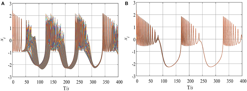
Figure 5. Time series of the network. (A) q = 14; (B) q = 0.9.

3.3. Complexity of the Network

The complexity analysis of networks is a new topic. Since the non-linear systems in the network can also generate time series, measurement of the complexity of the network is possible and necessary. For a given network, if the complexity of each node is different, this means that the states of nodes in the network are different. This provides a novel tool for the analysis of a network from a complexity point of view.

Here, the time series x_i (i = 1, 2, ⋯ , Num) from the network are employed to estimate the complexity of the network. Num is the number of nodes, and Num = 100. When the network has high complexity, the network is chaotic, or at least that the nodes in the network are not periodic or convergent. Meanwhile, if the complexity of each node is different, the state of each node is different. Thus, the chimera state or asynchronization exists in the network.

The steps for complexity measurement of the network are summarized as follows.

Step 1: Set the parameters and the coupling method of the network.

Step 2: Set j = 1, q = 0.7 and suppose that the complexity measure results are saved in matrix Comm.

Step 3: Estimate the complexity of time series x_i, and the complexity measure result is saved in Comm(j, i), where i = 1, 2, ⋯ , Num.

Step 4: Let j = j + 1, q = q + Δq, and repeat step 3 and step 4 until q = 1.

Step 5: Draw the contour plot of Comm.

In this paper, Δq = 0.003.

The complexity of the five cases is analyzed, and the results are shown in Figure 6. When q = 1, the network has higher complexity than in the other cases. According to Figure 6, the network has a chimera state or synchronization. Meanwhile, the complexity of the network in Case 1 is analyzed by varying the derivative order q from 0.7 to 1 with a step size of 0.003, and the results are shown in Figure 7. Figure 7 shows that the complexity of the network decreases with decrease in the derivative order q. In conclusion, when a chimera state exists, the system may have lower complexity measure values, which indicates that the network sacrifices its complexity for this state. Moreover, for this network with memristor, its complexity decreases with the fractional-order derivative order q.

FIGURE 6

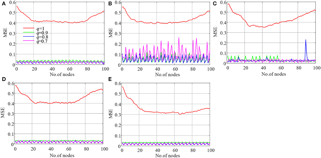
Figure 6. Results of complexity analysis of the network under different cases. (A) Case 1; (B) Case 2; (C) Case 3; (D) Case 4; (E) Case 5.

FIGURE 7

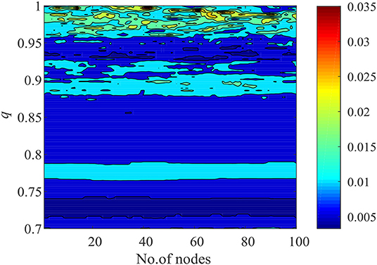
Figure 7. Results of complexity analysis of the network in Case 1 with different derivative order q values.

4. Conclusion

In this paper, the dynamics of an improved memristor neuron system are investigated, and a network of ring-coupled neurons is built with different coupling methods. The dynamics of the neural system are analyzed by means of LEs and bifurcation diagrams, and the network is investigated numerically. The conclusions of this paper are as follows.

1) The improved neural system has rich dynamics with the system parameter I_ext. When the system takes a smaller derivative order, less fluctuation occurs in the generated time series.

2) Five different coupling methods are introduced to connect the network, and numerical analysis results show that the chimera state exists in the network. When the derivative order q takes a smaller value, it is easier to observe a chimera state in the network.

3) Compared with the systems with q = 1, a network with q < 1 has much lower complexity. The fact is that, when there is a chimera state and synchronization, the complexity of the system is low. MSE is effective for estimating the complexity of the network, and it provides a new tool for dynamical analysis of the complex network.

Data Availability Statement

All datasets generated for this study are included in the article/supplementary material.

Author Contributions

The author confirms being the sole contributor of this work and has approved it for publication.

Funding

This work was supported by the Natural Science Foundation of China (Nos. 61901530 and 11747150), the China Postdoctoral Science Foundation (No. 2019M652791), and the Postdoctoral Innovative Talents Support Program (No. BX20180386).

Conflict of Interest

The author declares that the research was conducted in the absence of any commercial or financial relationships that could be construed as a potential conflict of interest.

Acknowledgments

The author would like to thank Dr. Sajad Jafari for his distinguished report regarding the network in our group and also the editor and the referees for their careful reading of this manuscript and valuable suggestions.

References

1. Dakiche N, Tayeb FBS, Slimani Y, Benatchba K. Tracking community evolution in social networks: a survey. Inform Process Manage. (2019) 56:1084–102. doi: 10.1016/j.ipm.2018.03.005

CrossRef Full Text | Google Scholar

2. Saleh M, Esa Y, Mohamed AA. Applications of complex network analysis in electric power systems. Energies. (2018) 11:1381. doi: 10.3390/en11061381

CrossRef Full Text | Google Scholar

3. Sun L, Yang Y, Fu X, Xu H, Liu W. Optimization of subway advertising based on neural networks. Math Probl Eng. (2020) 2020:18711423. doi: 10.1155/2020/1871423

CrossRef Full Text | Google Scholar

4. Xiang T, Wong KW, Liao X. Selective image encryption using a spatiotemporal chaotic system. Chaos. (2007) 17:023115. doi: 10.1063/1.2728112

PubMed Abstract | CrossRef Full Text | Google Scholar

5. Pathak J, Hunt BR, Girvan MK, Lu Z, Ott E. Model-free prediction of large spatiotemporally chaotic systems from data: a reservoir computing approach. Phys Rev Lett. (2018) 2:024102. doi: 10.1103/PhysRevLett.120.024102

PubMed Abstract | CrossRef Full Text | Google Scholar

6. Marre O, Boustani SE, Frégnac Y, Destexhe A. Prediction of spatiotemporal patterns of neural activity from pairwise correlations. Phys Rev Lett. (2009) 102:138101. doi: 10.1103/PhysRevLett.102.138101

PubMed Abstract | CrossRef Full Text | Google Scholar

7. Faghani Z, Arab Z, Parastesh F, Jafari S, Perc M, Slavinec M. Effects of different initial conditions on the emergence of chimera states. Chaos Solitons Fractals. (2018) 114:306–11. doi: 10.1016/j.chaos.2018.07.023

CrossRef Full Text | Google Scholar

8. Parastesh F, Jafari S, Azarnoush H, Hatef B, Bountis A. Imperfect chimeras in a ring of four-dimensional simplified Lorenz systems. Chaos Solitons Fractals. (2018) 110:203–8. doi: 10.1016/j.chaos.2018.03.025

CrossRef Full Text | Google Scholar

9. Rostami Z, Pham VT, Jafari S, Hadaeghi F, Ma J. Taking control of initiated propagating wave in a neuronal network using magnetic radiation. Appl Math Comput. (2018) 338:141–51. doi: 10.1016/j.amc.2018.06.004

CrossRef Full Text | Google Scholar

10. Parastesh F, Jafari S, Azarnoush H, Hatef B, Namazi H, Dudkowski D. Chimera in a network of memristor-based Hopfield neural network. Eur Phys J Spec Top. (2019) 228:2023–33. doi: 10.1140/epjst/e2019-800240-5

CrossRef Full Text | Google Scholar

11. Bera BK, Ghosh D, Lakshmanan M. Chimera states in bursting neurons. Phys Rev E. (2016) 93:012205. doi: 10.1103/PhysRevE.93.012205

PubMed Abstract | CrossRef Full Text | Google Scholar

12. Majhi S, Ghosh D. Alternating chimeras in networks of ephaptically coupled bursting neurons. Chaos. (2018) 28:083113. doi: 10.1063/1.5022612

PubMed Abstract | CrossRef Full Text | Google Scholar

13. Bao H, Zhang Y, Liu W, Bao B. Memristor synapse-coupled memristive neuron network: synchronization transition and occurrence of chimera. Nonlinear Dyn. (2020) 100:937–50. doi: 10.1007/s11071-020-05529-2

CrossRef Full Text | Google Scholar

14. Chen C, Bao H, Chen M, Xu Q, Bao B. Non-ideal memristor synapse-coupled bi-neuron Hopfield neural network: numerical simulations and breadboard experiments. AEU Int J Electron Commun. (2019) 111:152894. doi: 10.1016/j.aeue.2019.152894

CrossRef Full Text | Google Scholar

15. Kundu S, Bera BK, Ghosh D, Lakshmanan M. Chimera patterns in three-dimensional locally coupled systems. Phys Rev E. (2019) 99:022204. doi: 10.1103/PhysRevE.99.022204

PubMed Abstract | CrossRef Full Text | Google Scholar

16. Majhi S, Perc M, Ghosh D. Chimera states in a multilayer network of coupled and uncoupled neurons. Chaos. (2017) 27:073109. doi: 10.1063/1.4993836

PubMed Abstract | CrossRef Full Text | Google Scholar

17. Totz JF, Rode J, Tinsley MR, Showalter K, Engel H. Spiral wave chimera states in large populations of coupled chemical oscillators. Nat Phys. (2017) 14:282–5. doi: 10.1038/s41567-017-0005-8

CrossRef Full Text | Google Scholar

18. Makarov VV, Kundu S, Kirsanov DV, Frolov NS, Maksimenko VA, Ghosh D, et al. Multiscale interaction promotes chimera states in complex networks. Commun Nonlinear Sci Numer Simul. (2019) 71:118–29. doi: 10.1016/j.cnsns.2018.11.015

CrossRef Full Text | Google Scholar

19. Namba T, Rybka P. On viscosity solutions of space-fractional diffusion equations of caputo type. SIAM J Math Anal. (2020) 52:653–81. doi: 10.1137/19M1259316

CrossRef Full Text | Google Scholar

20. Kelly JF, Sankaranarayanan H, Meerschaert MM. Boundary conditions for two-sided fractional diffusion. J Comput Phys. (2019) 376:1089–107. doi: 10.1016/j.jcp.2018.10.010

CrossRef Full Text | Google Scholar

21. Shen L. Fractional derivative models for viscoelastic materials at finite deformations. Int J Solids Struct. (2020) 190:226–37. doi: 10.1016/j.ijsolstr.2019.10.025

CrossRef Full Text | Google Scholar

22. Chen L, Yi C, Wu R, Jian S, Ma T. Cluster synchronization in fractional-order complex dynamical networks. Phys Lett A. (2012) 376:2381–8. doi: 10.1016/j.physleta.2012.05.060

CrossRef Full Text | Google Scholar

23. Zhang S, Yu Y, Yu J. LMI conditions for global stability of fractional-order neural networks. IEEE Trans Neural Netw Learn Syst. (2017) 28:2423–33. doi: 10.1109/TNNLS.2016.2574842

PubMed Abstract | CrossRef Full Text | Google Scholar

24. Wang H, Yu Y, Wen G, Zhang S, Yu J. Global stability analysis of fractional-order Hopfield neural networks with time delay. Neurocomputing. (2015) 154:15–23. doi: 10.1016/j.neucom.2014.12.031

PubMed Abstract | CrossRef Full Text | Google Scholar

25. Farah FH, Grigorovsky V, Bardakjian BL. Coupled oscillators model of hyperexcitable neuroglial networks. Int J Neural Syst. (2019) 29:1850041. doi: 10.1142/S0129065718500417

PubMed Abstract | CrossRef Full Text | Google Scholar

26. He S, Sun K, Wang H. Synchronisation of fractional-order time delayed chaotic systems with ring connection. Eur Phys J Spec Top. (2016) 225:97–106. doi: 10.1140/epjst/e2016-02610-3

CrossRef Full Text | Google Scholar

27. Sommer C, German R, Dressler F. Bidirectionally coupled network and road traffic simulation for improved IVC analysis. IEEE Trans Mobile Comput. (2011) 10:3–15. doi: 10.1109/TMC.2010.133

CrossRef Full Text | Google Scholar

28. Pincus SM. Approximate entropy (ApEn) as a complexity measure. Chaos. (1995) 5:110–7. doi: 10.1063/1.166092

PubMed Abstract | CrossRef Full Text | Google Scholar

29. Chen W, Zhuang J, Yu W, Wang Z. Measuring complexity using FuzzyEn, ApEn, and SampEn. Med Eng Phys. (2009) 31:61–8. doi: 10.1016/j.medengphy.2008.04.005

PubMed Abstract | CrossRef Full Text | Google Scholar

30. Rosso OA, de Micco L, Larrondo HA, Martn MT, Plastino A. Generalized statistical complexity measure. Int J Bifurcation Chaos. (2010) 20:775–85. doi: 10.1142/S021812741002606X

CrossRef Full Text | Google Scholar

31. Enhua S, Zhijie C, Fanji G. Mathematical foundation of a new complexity measure. Appl Math Mech. (2005) 26:1188–196. doi: 10.1007/BF02507729

CrossRef Full Text | Google Scholar

32. Staniczenko PPA, Lee CF, Jones NS. Rapidly detecting disorder in rhythmic biological signals: a spectral entropy measure to identify cardiac arrhythmias. Phys Rev E. (2009) 79:011915. doi: 10.1103/PhysRevE.79.011915

PubMed Abstract | CrossRef Full Text | Google Scholar

33. Wang S, He S, Yousefpour A, Jahanshahi H, Repnik R, Perc M. Chaos and complexity in a fractional-order financial system with time delays. Chaos Solitons Fractals. (2020) 131:109521. doi: 10.1016/j.chaos.2019.109521

CrossRef Full Text | Google Scholar

34. He S, Banerjee S, Yan B. Chaos and Symbol Complexity in a Conformable Fractional-Order Memcapacitor System. Complexity. (2018) 2018:4140762. doi: 10.1155/2018/4140762

CrossRef Full Text | Google Scholar

35. Ma J, Tang J. A review for dynamics of collective behaviors of network of neurons. Sci China Technol Sci. (2015) 58:2038–45. doi: 10.1007/s11431-015-5961-6

CrossRef Full Text | Google Scholar

36. Carpinteri A, Mainardi F. Editors. Fractals and Fractional Calculus in Continuum Mechanics New York, NY: Springer. (1997). p. 291–348.

Google Scholar

37. Sun H, Abdelwahab A, Onaral B. Linear approximation of transfer function with a pole of fractional power. IEEE Trans Autom Control. (1984) 29:441–4.

Google Scholar

38. Danca MF, Kuznetsov NV. Matlab code for lyapunov exponents of fractional-order systems. Int J Bifurcation Chaos. (2018) 28:1850067. doi: 10.1142/S0218127418500670

CrossRef Full Text | Google Scholar

39. Wolf A, Swift JB, Swinney HL, Vastano JA. Determining lyapunov exponents from a time series. Phys D. (1985) 16:285–317.

Google Scholar

40. He S, Sun K, Wang H. Complexity analysis and DSP implementation of the fractional-order lorenz hyperchaotic system. Entropy. (2015) 17:8299–311. doi: 10.3390/e17127882

CrossRef Full Text | Google Scholar

41. Costa M, Goldberger AL, Peng CK. Multiscale entropy analysis of complex physiologic time series. Phys Rev Lett. (2002) 6:068102. doi: 10.1103/PhysRevLett.89.068102

PubMed Abstract | CrossRef Full Text | Google Scholar