Integrating Actin and Myosin II in a Viscous Model for Cell Migration

1. Introduction

Cell migration is fundamental in many biological processes and plays a key role in wound healing, immune response, development of embryos, inflammation, cancer invasion among others [1–6]. According to experimental observations, cell migration in eukaryotic cells is powered by actin-myosin system [7]. The actin cytoskeleton and its corresponding motor proteins play crucial role in cell movement. Actin is a polymer that can exist in two forms: F-actin and G-actin forms [1, 5, 6]. It converts from inactive state (G-actin) to active state (F-actin) through a process called actin polymerization and conversely from active state to inactive state through actin depolymerization [1, 6, 8]. The regulatory proteins are responsible for these actin polymerization-depolymerization processes [1, 8]. Actin polymerization promoting proteins such as nucleator proteins help in creating new actin filaments [8]. On the other hand, actin depolymerization factor such as cofilin is capable of binding to the actin filament causing it to disintegrate and form G-actin monomers [1, 8]. Actin filaments have two distinct ends: a plus end called barbed end which is a fast growing end and a minus end which is a slow growing end [7, 8]. Actin filaments can assemble structures forming networks and bundles through interaction with motor proteins [9, 10]. These structures produce cell protrusions called lamellipodia [6, 7, 11]. Actin cytoskeleton is therefore the main structure that contributes actively to force generation and therefore drives cell movement [6, 12].

Actin filament is responsible for force generations that drive cell migration through two major processes, namely: (i) rapid polymerization of actin network at the cell periphery through the growth of lamellipodia [5, 6, 13–15]. This leads to expansion of the plasma membrane and thus to the development of a contact area with the substrate and (ii) the development of stress fibers and networks that are contractile due to the action of motor proteins that tend to slide actin filaments relative to each other [6, 15]. The most abundant motor proteins is myosin II [9, 16]. Myosin II is known to bind to actin filaments in the cortex, crosslinking and contracting the actin filaments, causing cortical tension and mechanical resistance, which drives the cells' overall behavior. These active forces from polymerization of actin and contraction of stress fibers are eventually transmitted to substrates through adhesion sites, hence providing the necessary forces required for cell propulsion [1, 12]. Similarly, new actin polymerization occurs between the cortex and the membrane, giving rise to outward pressure-driven cell membrane pseudopod formation, while in other regions of the cell, cortical tension pulls along the rest of the cell body (through contractility). All these processes when combined appropriately lead to cell movement and deformation. Cells are however not limited to crawling as a means of migrating. It has been observed that cells can swim while freely suspended in a fluid [17–19]. Infact, neutrophils can migrate with little to no adhesion [20].

For many centuries, experimental biology has occupied the minds of many researchers in the quest to understand the complexity of cell motility. In recent decades, mathematical and computational modeling has rapidly become an essential research technique that has greatly contributed to the understanding of the subject of cell motility [4]. The advantage of computational modeling is that it can overcome intrinsic experimental limitations and therefore allow for virtual experiments which sometimes are impossible to carry out in reality. This allows experimentalists to probe and pause new experimental hypotheses. It is a fact that cell motility involves a large number of proteins that interact together in a complex way [21]. Proposing an accurate model to account for the vast molecular interactions involved in cell motility is therefore a non-trivial activity. It is also largely known that the interaction of actin with its associated proteins is usually a major factor in the derivation of models for cell motility [4]. Many models are built on the concept that cell motility is composed of the following stages: protrusion, adhesion and contraction [1]. The cell pushes out the front, then it assembles tight adhesions to the surface at the leading edge and weakens such adhesions at the rear and finally the cell develops contractions that pull the weakly adherent rear toward the strongly adhered front [4]. Hence, these involve biomechanical interactions which describe the dynamical behavior between intra- and extra-cellular processes to enable the cell to migrate.

There have been different strategies of modeling cell migration in the last several decades. The first modeling efforts were directed at quantifying actin treadmill and using thermodynamics to understand the nature and magnitude of the polymerization force [4]. These early works introduced fundamental ideas that are still used in developing complex models [4]. In [22], “Polymerization Brownian ratchet” model was proposed to describe actin polymerization as rigid mechanism which elongates by rectifying the Brownian motion of the membrane. According to this model, when the end of an actin filament comes into contact with a membrane, the membrane would diffuse away and therefore create a gap sufficient for monomers to be added. These ratchet models used differential-difference equations [4, 22]. Later in [23], an improvement was made to this model to consider the filaments as elastic springs whose behavior is a function of the bending modulus of the filament and the angle it makes with a load at its tip. The thermal fluctuations of actin filaments displaces the actin filaments from the membrane and creates a gap for the elongation of the filament [23]. This model was able to predict an optimal angle between the actin filament and the load for the effective force transmission. In [24], ratchet models underwent further development when it was suggested that some of the actin filaments are attached to the surface they push. This model, the ‘tethered ratchet’ model, explains the mechanism by assuming that the filament attach to the surface transiently, dissociating fast and growing freely until getting capped and losing contact with the surface altogether [24]. In [25–27], actin polymerization and depolymerization were treated as stochastic processes.

In [28], a mathematical model that describes key details of actin dynamics in protrusion associated with cell motility was developed. This model was based on the dendritic-nucleation hypothesis for lamellipodial protrusion in non-muscle cells such as Keratocytes. An output of the model was a relationship between the protrusion velocity and the number of filament barbed ends pushing the membrane. They observed that this relationship has a local maximum: too many barbed ends deplete the available monomer pool and too few are insufficient to generate protrusive force. Their result suggested that to achieve rapid motility, some tuning of parameters affecting actin dynamics must be operating in the cell [28].

Continuum models have also been developed to study cell motility. These models can be classified as moving boundary problems since a motile cell is a typical example of such a class of partial differential equations. In many cases, the models describing the biochemical interactions between the molecular species are coupled to a momentum balance law that accounts for the forces driving the migration of the cell. Examples of moving boundary problems for cell migration include (but are not limited to): a two-phase fluid model for cytosol and the actin network in [29], a one-dimensional viscoelastic model of the cytoplasm and active stress generation in [30], a one-dimensional model for the actin distribution and its reaction in [31], a two-dimensional elastic continuum model in [32] and a cytomechanical model that couples a force balance mechanical equation for actin network to a reaction-diffusion equation for actin [33]. This cytomechanical model was later extended in [34] where they used a cartesian coordinate system.

Another strategy is to use phase-field models as described in these works [35–43]. In [44], a Keratocyte cell was modeled as a two dimensional sheet with fixed area. The shape of the cell membrane was determined by the interactions of various forces including the surface tension, the bending forces and the pressure that constraints the cell area. In [35, 36], a phase-field model was used to simulate vesicles' deformation and tumbling while in [37, 38], the phase-field was used to study the three dimension deformation of a vesicle membrane using an energetic framework. An extension of this model to multi-component vesicles was studied in [39]. In [41], a phase-field model for the Keratocyte cell that couples actin flow and adhesion mechanism during cell migration was presented. In the model, both myosin II contraction and actin polymerization were treated as active stresses. The adhesion sites could switch between the gripping mode and the slipping mode and their dynamics were integrated with actin flow. They also included tension and bending forces at the membrane. The various forces involved in cell migration are then considered and translated into velocity which then evolve the cell shape. Most recently, Moure and Gomez [43] gave a comprehensive review of phase-field models of individual and collective cell migration. They showed individual cell migration in confined and fibrous environments that highlight the mechanochemical interplay between the cell and the extracellular environment. Phase-fields have been adopted as one plausible numerical approach for handling moving boundary problems by embedding the sharp moving interface into a higher space-dimension which is fixed and then defining a phase-field function that describes the location of the cell (typically, 1 inside the cell) and (0 outside). The advantages of employing phase-fields include (i) the reformulation of a moving boundary problem onto a stationary domain and (ii) the method allows for topological changes in cell shape (e.g., cell division). On the other hand, phase-fields have disadvantages in that (i) by embedding the model into a higher dimension, the problem is now solved on a higher space dimension with one further partial differential equation for the phase-field function which is used to track the moving cell within the stationary and rather large space domain, and that extra modeling is required if topological changes are to be prohibited (for example by including a volume constraint term in the momentum balance law for example). Furthermore, refined meshes must be employed to resolve the partial differential equations as the small interface width order parameter is taken small. In this study, we will resort to modeling the sharp interface rather than the diffuse-interface formulation, for the moving boundary problem which is embedded naturally in the two-space dimension where a momentum balance law model is posed.

There exists many other noteworthy studies that have been carried out to model cell motility. Recently, a multiscale computational model coupling fluid mechanics, solid mechanics, and pattern formation was developed to simulate fully 3D, pseudopod-driven motility of amoeboid cells through a fluid filled porous medium [20]. The results and analysis presented showed a strong coupling between cell deformability and ECM properties. In [45], both two and three dimensions (2D and 3D) cell motility models were simulated using an activator-inhibitor system coupled with an evolving surface finite element method. In [46], a phase-field model for a 3D amoeboid cell was studied, including an activator-inhibitor system to describe the cell biochemistry, transport equations to describe cytosolic biochemistry dynamics and hydrodynamic drag to describe adhesive forces. Simulations were performed in 2D for cells navigating around obstacles on a substrate and in 3D for cells in rigid periodic cylindrical fibrous networks. In [47], a 2D model of motile cells was developed using an immersed-boundary method that resolves cell deformation, internal and external fluid flow and a reaction-diffusion system in the entire volume of the cell while in [48], a 2D model also using an immersed-boundary method in which the cytoskeleton is represented as a dynamic network of springs immersed in a fluid was presented. In [49], a deformable cell driven under a prescribed axisymmetric oscillating force in an unbounded medium was considered. A phase field approach to simulate migration of neutrophils in 3D in response to external cues was presented in [50]. In [51], a moving mesh finite element method for the approximate solution of coupled bulk-surface reaction-diffusion equations on an evolving two dimensional domain was studied. They used a moving mesh partial differential equation and generated bulk and surface meshes. They applied the method to model the two-way interaction of a migrating cell with an external chemotactic field. In [52, 53], a Filament Based Lamellipodium Model (FBLM) which is a two-dimensional, anisotropic, two-phase model derived from microscopic description was studied. This model describes the actin network in terms of two transversal families of parallel filaments stabilized by cross-links and substrate adhesion. In [54], the FBLM was extended to investigate the effects of myosin polymers. The basic assumption here being that pairs of crossing actin filaments may be connected by myosin filaments.

Recently, Mackenzie et al. [55] investigated mass conservation property of a fully discrete finite element approximation of an ALE reformulation of a bulk-surface system on an evolving domain applied to a problem on cell polarization and chemotaxis on a moving domain. In this work, moving mesh methods were employed to move the internal mesh given the knowledge of the surface boundary through Dirichlet boundary conditions. In their work, the flow velocity generated by the force balance equation is assumed to be continuous across the boundary, thereby giving rise to global deformation of the mesh. Applications to cell polarization include the recent work by Cusseddu et al. [56] where the bulk-surface finite element method is used to generate numerical simulations over simple and complex geometries for the bulk-surface wave pinning model in 3-dimensions. In [57], a three-dimensional model for chemotactic motion of amoeboid cells was proposed. It accounted for the interactions between the extracellular substances, the membrane-bound proteins and the cytosolic components involved in the signaling pathway that lead to cell motility. Most recently, Moure and Gomez [58] studied the role of the cell nucleus in 2D cell migration where they used a computational model of fish keratocytes.

Our model is highly non-linear and is defined on a continuously evolving domain representing the cell. The non-linearity of the model makes it difficult to obtain analytical solutions. Numerical methods are therefore a good choice in solving these models. Numerical methods for partial differential equations consist of two parts: a space discretization to transform the system of partial differential equations into a system of ordinary differential equations and a time discretization to transform the system of ordinary differential equations into a system of linear or non-linear algebraic equations depending on the time discretisation scheme applied. Finally, techniques from numerical linear algebra can be employed to solve the resulting system of linear equations. For the system of non-linear equations, a linearization for the non-linear terms is required in order to use numerical linear algebra. Space discretization methods include (but are not limited to) finite differences [59, 60], finite elements [61–63], boundary elements [64] among other methods. The finite element method is well-known to handle complex and evolving cellular domains and can be easily generalized into multidimensions. It is a robust method that has been widely used to model cell motility and other problems involving reaction-diffusion equations in both stationary and continuously deforming domains [65–73].

Several time discretization have been used to obtain solutions for partial differential equations on both stationary and evolving domains. Fully explicit methods require very small time steps which result in computations that are expensive especially when it comes to multi-dimensions. Ruuth [74] presented different IMplicit-EXplicit (hence IMEX) schemes for solving reaction-diffusion systems on stationary domains, and their generalizations to growing domains were undertaken in [69]. The key essence of these schemes is that an implicit scheme is applied to approximate the diffusive term and an explicit scheme is used to approximate the reaction kinetics. The IMEX schemes presented in [69, 74] include a first order semi-implicit backward differentiation formula (1-SBDF) which applies a backward differentiation formula to the diffusive term, Crank-Nicolson, Adams-Bashforth (CNAB) which applies Crank-Nicolson to the diffusive term and second order Adams-Bashforth to the reaction terms, Crank-Nicolson Leap Frog (CNLF) which applies something similar to Crank-Nicolson to the diffusive term and a leap frog to the reaction terms, the second order semi-implicit backward differentiation formula (2-SBDF), which applies a second order formula to the diffusive term, the third order semi-implicit backward differentiation formula (3-SBDF) which applies a third order formula to the diffusive term and the first order backward Euler finite difference scheme (1-SBEM) which treats both the diffusive term and linear part of the reaction term implicitly and non-linear part of the reaction semi-implicitly. We note that the 1-SBDF, the 2-SBDF and the 3-SBDF schemes are known to give strong decay of high frequency error components while unfortunately the CNAB and CNLF schemes are known to give a weak damping of high frequency error components [74]. From numerical experiments, the 2-SBDF is recommended as a good scheme to many two dimensional problems [69, 74]. Recently, Madzvamuse and Chung [73] used a fully implicit scheme to solve a system of bulk-surface coupled reaction-diffusion equations. This scheme requires some special linearization techniques as shown in [73]. For this work, it is sufficient to apply the second order semi-implicit backward differentiation formula (2-SBDF) to discretize in time, the system of reaction-diffusion equations on the migrating cell, while a first order forward Euler's formula is used to update the moving mesh.

The focus of this work is to incorporate both actin and myosin II as well as convective terms in a reaction-diffusion model for cell motility where the models are posed on a moving domain with a sharp moving interface boundary. Our model involves a reaction-diffusion equation that considers myosin II activity in driving cell motion. We consider generalized reaction kinetics to model polymerization and depolymerization processes, where the kinetics take into account positive feedback from actin filaments. We formulate a system of reaction-diffusion equations to describe the actomyosin spatiotemporal dynamics during cell migration that in turn drives the actin filament structure here described by a viscous mechanical model in the absence of cell membrane and adhesion forces, hence our model is simpler than its phase-field counterpart [41]. Since the actomyosin system is always contained inside the cell and does not cross the cell boundary, we consider zero-flux boundary conditions. These boundary conditions ensure that biochemical concentrations do not flow across the boundary allowing for self-organization of the molecular species within the cell. The proposed framework is an alternative numerical or computational approach where phase-fields have been employed to offer numerical solutions on stationary domains which embed the migrating cell domain in a higher space-dimension [41, 75]. This entails that we do not need to solve an extra equation for the phase-field function that is used to track the moving boundary. Hence, our main contribution is the development of an evolving finite element method for solving the moving boundary problem posed on its physical domain that is moving. We note that in the literature, different numerical methods have been adopted but the use of evolving finite elements for solving models that couple biomechanics with biochemistry are very few [71, 72]. Furthermore, there is no need to employ refined mesh around the interface to resolve the numerical solution of the moving boundary problem within the small region encompassing the moving interface [76]. Our model is able to show expansion, contraction and deformation of the cell following actomyosin activity, with no substantial changes in shape. Our results are consistent with biological observations involving the migration of Keratocytes which are known to migrate with minimal changes in shape. Our simpler model captures the symmetry breaking process from a unit-circle shape to a polarized shape with a well-defined front and back in the absence of membrane and adhesion forces [56].

Hence, the structure of this article is as follows: in section 2, we present the model equations for cell migration and carry out non-dimensionalization of the model system. In section 3, we present a detailed moving finite element method (also now known as the evolving finite element method) and discretize in time to arrive at fully discrete equations. We also describe how we solve the discrete system of equations. We present various numerical results from our simulations in section 4. Finally, we conclude and outline future research directions in section 5.

2. A Viscous Model for Cell Migration

We model the network of actin filaments in the cell as a viscous gel with active stresses generated from the action of actin and myosin II. The viscous model for cell migration considered in this work comprises of a system of reaction-advection-diffusion equations coupled to a force balance mechanical equation. Our current model does not include cellular adhesion and membrane forces that is brought about by tension and bending, which were considered in [41, 75]. While adhesion plays an important role in cell migration, it has been shown that motility can occur with nearly no adhesion for example during cell swimming. Infact, neutrophils can migrate with little to no adhesion [20].

2.1. Model Formulation

Let ${\Omega }_t\subset {ℝ}^2$ be a simply connected, bounded and continuously deforming domain representing the cell shape at time t ∈ (0, T], T > 0 and ∂Ω_t be the boundary of the cell with normal n = (n₁, n₂) at a point x(t). At any point x(t) = (x(t), y(t)) ∈ Ω_t, let ρ_m = ρ_m(x(t), t) be the myosin II concentration, ρ_a = ρ_a(x(t), t) be the F-actin concentration in Ω_t and β = β(x(t), t) be the actin flow velocity which we assume is identical to the mesh/domain velocity of the cell. It must be noted that other works exist [51, 55] where the flow velocity is different from the mesh velocity. We note that points x(t) move with velocity β(x(t), t), and that this velocity also describes the change of shape as it is also the velocity of the boundary points, through the continuity of boundary conditions. The model we consider is a simpler version of previous models for cell migration [41, 75, 77] and takes into account biochemical and mechanical structure of the cell. It is a viscous model that couples a force balance mechanical equation to reaction-advection-diffusion equations for actin and myosin II as summarized below.

$\begin{array}{ll}\nabla ·\left({\sigma }_{\nu }(\text{x},t)+{\sigma }_{myo}(\text{x},t)+{\sigma }_{poly}(\text{x},t)\right)=0,\text{x}\in {\Omega }_t,t\in (0,T],& (\mathrm{2.1a})\end{array}$

$\begin{array}{ll}\frac{\partial {\rho }_m}{\partial t}+\nabla ·({\rho }_m\beta )=\nabla ·\left(D_m({\rho }_a)\nabla {\rho }_m\right),\text{x}\in {\Omega }_t,t\in (0,T],& (\mathrm{2.1b})\end{array}$

$\begin{array}{ll}\frac{\partial {\rho }_a}{\partial t}+\nabla ·({\rho }_a\beta )=D_a\Delta {\rho }_a+f({\rho }_a,{\rho }_a^{cyt}),\text{x}\in {\Omega }_t,t\in (0,T],& (\mathrm{2.1c})\end{array}$

with initial conditions

$\begin{array}{ll}{\rho }_m(\text{x},0)={\rho }_m^0(\text{x}),\text{x}\in {\Omega }_0,& (\mathrm{2.2a})\end{array}$

$\begin{array}{ll}{\rho }_a(\text{x},0)={\rho }_a^0(\text{x}),\text{x}\in {\Omega }_0.& (\mathrm{2.2b})\end{array}$

To close the system, we apply zero-flux and stress-free boundary conditions given by

$\begin{array}{ll}\frac{\partial {\rho }_m}{\partial \text{n}}=\frac{\partial {\rho }_a}{\partial \text{n}}=0,\text{x}\in \partial {\Omega }_t,t\in (0,T],& (\mathrm{2.3a})\end{array}$

$\begin{array}{ll}{\sigma }_{\nu }·\text{n}=0,\text{x}\in \partial {\Omega }_t,t\in (0,T],& (\mathrm{2.3b})\end{array}$

and the terms in the reaction-diffusion system given by

$\begin{array}{l}f({\rho }_a,{\rho }_a^{cyt})=k_b\left(\frac{{\rho }_a^2}{K_a^2+{\rho }_a^2}+k_a\right){\rho }_a^{cyt}-k_c{\rho }_a,\\ {\rho }_a^{cyt}=\frac{{\rho }_a^{tot}-{\displaystyle {\int }_{{\Omega }_t}}{\rho }_{a}d{\Omega }_t}{{\displaystyle {\int }_{{\Omega }_t}}d{\Omega }_t}\\ \text{and }{D}_m({\rho }_a)=\frac{D_m^0}{1+\frac{{\rho }_a}{K_D}}.\end{array}$

The terms ∇ · (ρ_mβ) and ∇ · (ρ_aβ) denote the convective and dilution processes due to cell movement and growth and these were not considered in some previous studies of this nature, for example [33, 77]. Next, we introduce the quantities $\frac{D{\rho }_m}{Dt}$ and $\frac{D{\rho }_a}{Dt}$, known as the material derivatives of ρ_m and ρ_a and these will be used throughout the sequel. The material derivatives are defined as

$\begin{array}{l}\frac{D{\rho }_m}{Dt}=\frac{\partial {\rho }_m}{\partial t}+\beta ·\nabla {\rho }_m\text{ and }\frac{D{\rho }_a}{Dt}=\frac{\partial {\rho }_a}{\partial t}+\beta ·\nabla {\rho }_a,\end{array}$

respectively [62]. The reaction kinetics for the actin equation, $f({\rho }_a,{\rho }_a^{cyt})$, depends on the F-actin ρ_a and G-actin ${\rho }_a^{cyt}$ concentrations [41, 75] and that G-actin is assumed to be well mixed inside the cell [8]. Diffusion for myosin II D_m(ρ_a) is assumed to depend on the F-actin concentration in such a way that diffusion is reduced when F-actin concentration increases [75]. We note that in the absence of F-actin, myosin II diffuses with the constant rate $D_m^0$. The constant D_a is a positive diffusion coefficient for F-actin [41, 75]. The terms σ_myo(x, t), σ_ν(x, t), and σ_poly(x, t) are the myosin II driven contractile, viscous, and actin generated stresses, respectively, and are given by [41]

$\begin{array}{l}{\sigma }_{myo}(\text{x},t)={\eta }_m^0{\rho }_m(\text{x},t)\text{I},{\eta }_m^0\in {ℝ}^{+},\\ {\sigma }_{\nu }(\text{x},t)=\frac{{\nu }_0}{2}\left(\nabla \beta (\text{x},t)+{(\nabla \beta (\text{x},t))}^T\right),{\nu }_0\in {ℝ}^{+}\\ \text{\hspace{0.17em}and }{\sigma }_{poly}(\text{x},t)=-{\eta }_a^0{\rho }_a(\text{x},t)\delta (l)\text{I},{\eta }_a^0\in {ℝ}^{+},\end{array}$

where $\frac{1}{2}\left(\nabla \beta (\text{x},t)+{(\nabla \beta (\text{x},t))}^T\right)$ represents the rate of strain tensor, I is the identity tensor in two dimensions and δ(l) labels the cell periphery. The constants ν₀, ${\eta }_m^0$, and ${\eta }_a^0$ are the shear viscosity coefficient, myosin II contraction coefficient, and F-actin protrusion coefficient, respectively. Table 1 shows a list of all the model parameters used. We have prescribed zero-flux boundary conditions to model spontaneous random cell migration and set initial conditions for both actin and myosin II. The polymerization stress only acts in the cell periphery. In order to describe this stress, we will assume an initial domain of a disk and specify that σ_poly(x, t) only acts in the region which is some distance l from the centre of the disk domain. With this we define the function δ(l) to be of the form

$\delta (l)=\{\begin{array}{l}1\text{ if the point }\text{x}\text{ is such its distance from the origin of}\hfill \\ \text{ the disk is more than }l,\hfill \\ 0\text{ otherwise}.\hfill \end{array}$

This means that far from the cell periphery, only the contractile stress acts on the cell and close to the cell periphery both the contractile and the actin generated polymerization stresses act on the cell.

TABLE 1

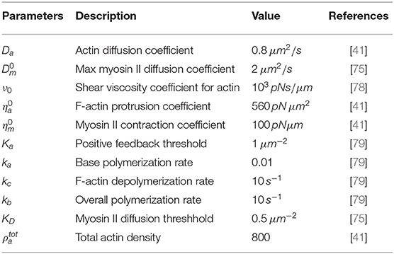
Table 1. Dimensional parameters and their values as used in the model.

Remark

It must be noted that the model system (2.1a-2.1c), although posed on a two-dimensional deforming domain, generalizes immediately to three-dimensional volumes. Similarly, the application of the evolving finite element method to the model system also generalizes to three-dimensional volumes.

2.2. The Non-dimensionalized Model

We introduce non-dimensional rescaled variables as follows:

$\begin{array}{l}\widehat{{\rho }_m}=\frac{{\rho }_m}{K_a},\widehat{{\rho }_a}=\frac{{\rho }_a}{K_a},\widehat{\beta }=\frac{\beta }{k_{b}R},\widehat{t}=t{k}_b,\end{array}$

where R is the scaling factor for length. For notational simplicity, we drop all hats and the resulting non-dimensionalized viscous model for cell migration with non-dimensionalized parameters given in Table 2 therefore reads

$\begin{array}{ll}\nabla ·\left({\sigma }_{\nu }(\text{x},t)+{\sigma }_{myo}(\text{x},t)+{\sigma }_{poly}(\text{x},t)\right)=0,\text{x}\in {\Omega }_t,t\in (0,T],& (\mathrm{2.4a})\end{array}$

$\begin{array}{ll}\frac{\partial {\rho }_m}{\partial t}+\nabla ·({\rho }_m\beta )=\nabla ·\left(\left(\frac{1}{1+a{\rho }_a}\right)\nabla {\rho }_m\right),\text{x}\in {\Omega }_t,t\in (0,T],& (\mathrm{2.4b})\end{array}$

$\begin{array}{l}\frac{\partial {\rho }_a}{\partial t}+\nabla ·({\rho }_a\beta )=d\Delta {\rho }_a+\left(\frac{{\rho }_a^2}{1+{\rho }_a^2}+k_a\right){\rho }_a^{cyt}\\ \begin{array}{l}-e{\rho }_a,\text{x}\in {\Omega }_t,t\in (0,T],\end{array}& (\mathrm{2.4c})\end{array}$

with initial conditions given by

$\begin{array}{ll}{\rho }_m(\text{x},0)={\rho }_m^0(\text{x}),\text{x}\in {\Omega }_0,& (\mathrm{2.5a})\end{array}$

$\begin{array}{ll}{\rho }_a(\text{x},0)={\rho }_a^0(\text{x}),\text{x}\in {\Omega }_0,& (\mathrm{2.5b})\end{array}$

and boundary conditions

$\begin{array}{ll}\frac{\partial {\rho }_a}{\partial \text{n}}=\frac{\partial {\rho }_m}{\partial \text{n}}=0,\text{x}\in {\partial \Omega }_t,t\in (0,T],& (\mathrm{2.6a})\end{array}$

$\begin{array}{ll}{\sigma }_{\nu }·\text{n}=0,\text{x}\in {\partial \Omega }_t,t\in (0,T],& (\mathrm{2.6b})\end{array}$

with

$\begin{array}{l}{\rho }_a^{cyt}(t)=\frac{{\rho }_a^{tot}-{\displaystyle {\int }_{{\Omega }_t}}{\rho }_{a}d{\Omega }_t}{{\displaystyle {\int }_{{\Omega }_t}}d{\Omega }_t},\\ {\sigma }_{myo}(\text{x},t)={\eta }_1{\rho }_m(\text{x},t)\text{I},{\eta }_1\in {ℝ}^{+},\\ {\sigma }_{\nu }(\text{x},t)=\nabla \beta (\text{x},t)+{(\nabla \beta (\text{x},t))}^T,\\ {\sigma }_{poly}(\text{x},t)=-{\eta }_2{\rho }_a(\text{x},t)\delta (l)\text{I},{\eta }_2\in {ℝ}^{+},\end{array}$

where ρ_a, ρ_m, and β are the dependent variables for this model. The initial domain is now a disk with radius r = 1. Since the polymerization force is assumed to work only in the periphery of the cell [8], we let it act only in the region l ≥ 0.8. The delta function δ(l) ensures that polymerization force only act in this region.

TABLE 2

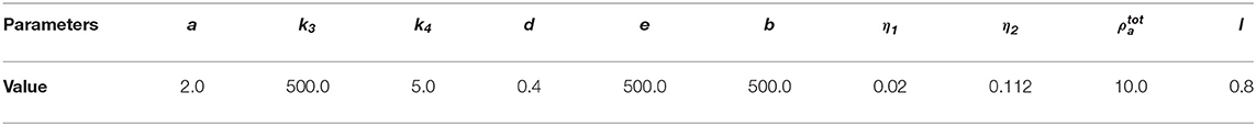
Table 2. Non-dimensional parameter values for the non-dimensionalized viscous model.

3. The Evolving Finite Element Method for Simulating the Viscous Model

We employ the evolving (moving grid) finite element method to derive a numerical scheme for the non-dimensionalized viscous model for cell migration. We use the evolving finite elements [61] to discretize the viscous model in space and apply a second order semi-implicit backward differentiation formula (2-SBDF) [69, 74] to discretise the system of reaction-diffusion equations in time. To update the mesh after solving the equations in each timestep, we apply a first order forward Euler method. Convergence analysis for the reaction-diffusion system was undertaken on stationary domains (in the absence of the viscous model) and second-order convergence was established (results not shown). Demonstrating convergence for the full viscous model is an open problem due to the non-linear coupling between the mechanical and biochemical models. The evolving finite element method is an efficient method that is able to deal with complex and irregular geometries and has been widely used for growing and deforming domains [67–69, 72]. From numerical experiments, the 2-SBDF is recommended as an efficient numerical time integrating scheme for reaction-diffusion equations. For more illustration on these, see for example [74]. Further information on the implementation of the evolving finite element method and time-integration can be found in [80].

The evolving finite element method therefore involves the following steps: derivation of weak formulation of the partial differential equations, the finite element spatial discretization to obtain a system of semi-discrete equations and a temporal discretization to obtain fully discrete system of equations.

3.1. Derivation of the Weak Formulation

3.1.1. Weak Formulation of the Reaction-Advection-Diffusion Equations

Reaction-advection-diffusion equations for myosin II and F-actin are, respectively, given by

$\begin{array}{ll}\frac{\partial {\rho }_m}{\partial t}+\nabla ·({\rho }_m\beta )=\nabla ·\left(\frac{1}{1+a{\rho }_a}\nabla {\rho }_m\right),& (\mathrm{3.1a})\end{array}$

$\begin{array}{ll}\frac{\partial {\rho }_a}{\partial t}+\nabla ·({\rho }_a\beta )=d\Delta {\rho }_a+\left(\frac{k_3{\rho }_a^2}{1+{\rho }_a^2}+k_4\right){\rho }_a^{cyt}-e{\rho }_a,& (\mathrm{3.1b})\end{array}$

where ρ_m = ρ_m(x(t), t) and ρ_a = ρ_a(x(t), t) are the myosin II and F-actin concentrations, respectively, and β = β(x(t), t) = (β₁, β₂) is the flow velocity of the actin network. Here, we note that the reaction kinetics of F-actin only depends on ρ_a variable and no reaction kinetics for the myosin II equation.

In order to obtain the weak formulation, we will rearrange (3.1a) and (3.1b). We apply product rule for gradient to the advection terms and write the equations as

$\begin{array}{ll}\frac{\partial {\rho }_m}{\partial t}+\beta ·\nabla {\rho }_m+{\rho }_m\nabla ·\beta =\nabla ·\left(\frac{1}{1+a{\rho }_a}\nabla {\rho }_m\right),& (\mathrm{3.2a})\end{array}$

$\begin{array}{l}\frac{\partial {\rho }_a}{\partial t}+\beta ·\nabla {\rho }_a+{\rho }_a\nabla ·\beta =d\Delta {\rho }_a\\ \begin{array}{l}+\left(\frac{k_3{\rho }_a^2}{1+{\rho }_a^2}+k_4\right){\rho }_a^{cyt}-e{\rho }_a.\end{array}& (\mathrm{3.2b})\end{array}$

We recall that the quantities $\frac{\partial {\rho }_m}{\partial t}+\beta ·\nabla {\rho }_m$ and $\frac{\partial {\rho }_a}{\partial t}+\beta ·\nabla {\rho }_a$ are called material derivatives of ρ_m and ρ_a and are written as $\frac{D{\rho }_m}{Dt}=\frac{\partial {\rho }_m}{\partial t}+\beta ·\nabla {\rho }_m$ and $\frac{D{\rho }_a}{Dt}=\frac{\partial {\rho }_a}{\partial t}+\beta ·\nabla {\rho }_a$. Now, using this definition for material derivatives above, we write (3.2a) and (3.2b) as

$\begin{array}{ll}\frac{D{\rho }_m}{Dt}+{\rho }_m\nabla ·\beta =\nabla ·\left(\frac{1}{1+a\rho }\nabla {\rho }_m\right),& (\mathrm{3.3a})\end{array}$

$\begin{array}{ll}\frac{D{\rho }_a}{Dt}+{\rho }_a\nabla ·\beta =d\Delta {\rho }_a+\left(\frac{k_3{\rho }_a^2}{1+{\rho }_a^2}+k_4\right){\rho }_a^{cyt}-e{\rho }_a,& (\mathrm{3.3b})\end{array}$

respectively. In order to obtain the weak formulations, we multiply (3.3a) and (3.3b) by sufficiently smooth functions ψ₁(x, t), ψ₂(x, t) and integrate using Green's formula [81, 82] in the domain Ω_t and use the boundary conditions $\frac{\partial {\rho }_a}{\partial \text{n}}=\frac{\partial {\rho }_m}{\partial \text{n}}=0$. This yields

$\begin{array}{l}{\displaystyle {\int }_{{\Omega }_t}}\left({\psi }_1\frac{D{\rho }_m}{Dt}+{\psi }_1{\rho }_m\nabla ·\beta \right)d{\Omega }_t\\ \begin{array}{l}=-{\displaystyle {\int }_{{\Omega }_t}}\frac{1}{1+a{\rho }_a}\nabla {\psi }_1·\nabla {\rho }_{m}d{\Omega }_t,\end{array}& (\mathrm{3.4a})\end{array}$

$\begin{array}{l}{\displaystyle {\int }_{{\Omega }_t}}\left({\psi }_2\frac{D{\rho }_a}{Dt}+{\psi }_2{\rho }_a\nabla ·\beta \right)d{\Omega }_t\\ =-{\displaystyle {\int }_{{\Omega }_t}}d\nabla {\psi }_2·\nabla {\rho }_{a}d{\Omega }_t\\ \begin{array}{l}+{\displaystyle {\int }_{{\Omega }_t}}{\psi }_2\left(\left(\frac{k_3{\rho }_a^2}{1+{\rho }_a^2}+k_4\right){\rho }_a^{cyt}-e{\rho }_a\right)d{\Omega }_t.\end{array}& (\mathrm{3.4b})\end{array}$

We further use the product rule for the time derivatives in the Equations (3.4a) and (3.4b) and write

$\begin{array}{l}{\displaystyle {\int }_{{\Omega }_t}}\left(\frac{D({\psi }_1{\rho }_m)}{Dt}-{\rho }_m\frac{D{\psi }_1}{Dt}+{\psi }_1{\rho }_m\nabla ·\beta \right)d{\Omega }_t\\ \begin{array}{l}=-{\displaystyle {\int }_{{\Omega }_t}}\frac{1}{1+a{\rho }_a}\nabla {\psi }_1·\nabla {\rho }_{m}d{\Omega }_t,\end{array}& (\mathrm{3.5a})\end{array}$

$\begin{array}{l}{\displaystyle {\int }_{{\Omega }_t}}\left(\frac{D({\psi }_2{\rho }_a)}{Dt}-{\rho }_a\frac{D{\psi }_2}{Dt}+{\psi }_2{\rho }_a\nabla ·\beta \right)d{\Omega }_t\\ =-{\displaystyle {\int }_{{\Omega }_t}}d\nabla {\psi }_2·\nabla {\rho }_{a}d{\Omega }_t\\ \begin{array}{l}+{\displaystyle {\int }_{{\Omega }_t}}{\psi }_2\left(\left(\frac{k_3{\rho }_a^2}{1+{\rho }_a^2}+k_4\right){\rho }_a^{cyt}-e{\rho }_a\right)d{\Omega }_t.\end{array}& (\mathrm{3.5b})\end{array}$

Finally Reynold's transport theorem [83] gives

$\begin{array}{l}\frac{d}{dt}{\displaystyle {\int }_{{\Omega }_t}}{\psi }_1{\rho }_{m}d{\Omega }_t-{\displaystyle {\int }_{{\Omega }_t}}{\rho }_m\frac{D{\psi }_1}{Dt}d{\Omega }_t\\ \begin{array}{l}=-{\displaystyle {\int }_{{\Omega }_t}}\frac{1}{1+a{\rho }_a}\nabla {\psi }_1·\nabla {\rho }_{m}d{\Omega }_t,\end{array}& (\mathrm{3.6a})\end{array}$

$\begin{array}{l}\frac{d}{dt}{\displaystyle {\int }_{{\Omega }_t}}{\psi }_2{\rho }_{a}d{\Omega }_t-{\displaystyle {\int }_{{\Omega }_t}}{\rho }_a\frac{D{\psi }_2}{Dt}d{\Omega }_t\\ =-{\displaystyle {\int }_{{\Omega }_t}}d\nabla {\psi }_2·\nabla {\rho }_{a}d{\Omega }_t\\ \begin{array}{l}+{\displaystyle {\int }_{{\Omega }_t}}{\psi }_2\left(\left(\frac{k_3{\rho }_a^2}{1+{\rho }_a^2}+k_4\right){\rho }_a^{cyt}-e{\rho }_a\right)d{\Omega }_t.\end{array}& (\mathrm{3.6b})\end{array}$

3.1.2. Weak Formulation of the Force Balance Equation

The force balance equation on an evolving domain Ω_t representing the cell is given by

$\begin{array}{ll}\{\begin{array}{l}\nabla ·\left({\sigma }_{\nu }(\text{x},t)+{\sigma }_{myo}(\text{x},t)+{\sigma }_{poly}(\text{x},t)\right)=0,\text{x}\in {\Omega }_t,t\in (0,T],\hfill \\ {\sigma }_{\nu }·\text{n}=0,\text{x}\in \partial {\Omega }_t,t\in (0,T],\hfill \end{array}& (3.7)\end{array}$

where σ_ν(x, t), σ_myo(x, t), and σ_poly(x, t) are the viscous, myosin II driven, and F-actin generated stresses, respectively. In order to write the weak formulation of the force balance above, we first decouple the stresses into x and y directions as follows.

$\begin{array}{ll}\{\begin{array}{l}\begin{array}{l}{\sigma }_{\nu }(\text{x},t)=\left(\begin{array}{cc}2\frac{\partial {\beta }_1}{\partial x}& \left(\frac{\partial {\beta }_2}{\partial x}+\frac{\partial {\beta }_1}{\partial y}\right)\\ \left(\frac{\partial {\beta }_2}{\partial x}+\frac{\partial {\beta }_1}{\partial y}\right)& 2\frac{\partial {\beta }_2}{\partial y}\end{array}\right),\hfill \\ {\sigma }_{myo}(\text{x},t)=\left(\begin{array}{cc}{\eta }_1{\rho }_m& 0\\ 0& {\eta }_1{\rho }_m\end{array}\right),\hfill \\ {\sigma }_{poly}(\text{x},t)=\left(\begin{array}{cc}-{\eta }_2{\rho }_a\delta (l)& 0\\ 0& -{\eta }_2{\rho }_a\delta (l)\end{array}\right).\hfill \end{array}\hfill \end{array}& (3.8)\end{array}$

The force balance equation in x and y directions is therefore

$\begin{array}{l}\frac{\partial }{\partial x}\left(2\frac{\partial {\beta }_1}{\partial x}\right)+\frac{\partial }{\partial y}\left(\frac{\partial {\beta }_2}{\partial x}+\frac{\partial {\beta }_1}{\partial y}\right)+\frac{\partial ({\eta }_1{\rho }_m)}{\partial x}\\ \begin{array}{l}-\frac{\partial }{\partial x}\left({\eta }_2{\rho }_a\delta (l)\right)=0,\end{array}& (\mathrm{3.9a})\end{array}$

$\begin{array}{l}\frac{\partial }{\partial x}\left(\frac{\partial {\beta }_2}{\partial x}+\frac{\partial {\beta }_1}{\partial y}\right)+\frac{\partial }{\partial y}\left(2\frac{\partial {\beta }_2}{\partial y}\right)+\frac{\partial ({\eta }_1{\rho }_m)}{\partial y}\\ \begin{array}{l}-\frac{\partial }{\partial y}\left({\eta }_2{\rho }_a\delta (l)\right)=0.\end{array}& (\mathrm{3.9b})\end{array}$

We then multiply the decoupled equations (3.9a) and (3.9b) by sufficiently smooth functions ψ₃, ψ₄, respectively, use Green's formula to integrate in the domain and apply the stress free boundary condition given. The boundary terms will vanish and the weak formulation thus reads: find ${\beta }_1(\text{x}(t),t),{\beta }_2(\text{x}(t),t)\in {\text{H}}^1({\Omega }_t)$ such that

$\begin{array}{l}{\displaystyle {\int }_{{\Omega }_t}}\left(2\frac{\partial {\psi }_3}{\partial x}\left(\frac{\partial {\beta }_1}{\partial x}\right)+\frac{\partial {\psi }_3}{\partial y}\left(\frac{\partial {\beta }_2}{\partial x}+\frac{\partial {\beta }_1}{\partial y}\right)\right)d{\Omega }_t\\ \begin{array}{l}={\displaystyle {\int }_{{\Omega }_t}}{\psi }_3\left(\frac{\partial f}{\partial x}\right)d{\Omega }_t,\end{array}& (\mathrm{3.10a})\end{array}$

$\begin{array}{l}{\displaystyle {\int }_{{\Omega }_t}}\left(\frac{\partial {\psi }_4}{\partial x}\left(\frac{\partial {\beta }_2}{\partial x}+\frac{\partial {\beta }_1}{\partial y}\right)+2\frac{\partial {\psi }_4}{\partial y}\left(\frac{\partial {\beta }_2}{\partial y}\right)\right)d{\Omega }_t\\ \begin{array}{l}={\displaystyle {\int }_{{\Omega }_t}}{\psi }_4\left(\frac{\partial f}{\partial y}\right)d{\Omega }_t,\end{array}& (\mathrm{3.10b})\end{array}$

for sufficiently smooth functions ρ₃, ρ₄, where f = δ(l)η₂ρ_a − η₁ρ_m.

We find it convenient to rewrite the right hand sides of equations (3.10a) and (3.10b) such that we have the derivatives of the shape function ρ₃ and ρ₄ instead of function f which depends on the solution values. Applying Green's Theorem [82] to equations (3.10a) and (3.10b) gives

$\begin{array}{l}{\displaystyle {\int }_{{\Omega }_t}}\left(2\frac{\partial {\psi }_3}{\partial x}\left(\frac{\partial {\beta }_1}{\partial x}\right)+\frac{\partial {\psi }_3}{\partial y}\left(\frac{\partial {\beta }_2}{\partial x}+\frac{\partial {\beta }_1}{\partial y}\right)\right)d{\Omega }_t=\\ \begin{array}{l}-{\displaystyle {\int }_{{\Omega }_t}}f\frac{\partial {\psi }_3}{\partial x}d{\Omega }_t+{\displaystyle {\int }_{\partial {\Omega }_t}}\left(n_{1}f{\psi }_3\right)dS,\end{array}& (\mathrm{3.11a})\end{array}$

$\begin{array}{l}{\displaystyle {\int }_{{\Omega }_t}}\left(\frac{\partial {\psi }_4}{\partial x}\left(\frac{\partial {\beta }_2}{\partial x}+\frac{\partial {\beta }_1}{\partial y}\right)+2\frac{\partial {\psi }_4}{\partial y}\left(\frac{\partial {\beta }_2}{\partial y}\right)\right)d{\Omega }_t=\\ \begin{array}{l}-{\displaystyle {\int }_{{\Omega }_t}}f\frac{\partial {\psi }_4}{\partial y}d{\Omega }_t+{\displaystyle {\int }_{\partial {\Omega }_t}}\left(n_{2}f{\psi }_4\right)dS,\end{array}& (\mathrm{3.11b})\end{array}$

where dS is the surface element and n = (n₁, n₂) is the outward unit normal to the boundary.

3.1.3. Weak Formulation of the Coupled Problem

The weak formulation for the coupled problem is summarized as follows:

find ${\rho }_m(\text{x}(t),t),{\rho }_a(\text{x}(t),t),{\beta }_1(\text{x}(t),t),{\beta }_2(\text{x}(t),t)\in {\text{H}}^1({\Omega }_t)$ such that

$\begin{array}{l}\frac{d}{dt}{\displaystyle {\int }_{{\Omega }_t}}{\psi }_1{\rho }_{m}d{\Omega }_t-{\displaystyle {\int }_{{\Omega }_t}}{\rho }_m\frac{D{\psi }_1}{Dt}d{\Omega }_t\\ \begin{array}{l}=-{\displaystyle {\int }_{{\Omega }_t}}\frac{1}{1+a{\rho }_a}\nabla {\psi }_1·\nabla {\rho }_{m}d{\Omega }_t,\end{array}& (3.12)\end{array}$

$\begin{array}{l}\frac{d}{dt}{\displaystyle {\int }_{{\Omega }_t}}{\psi }_2{\rho }_{a}d{\Omega }_t-{\displaystyle {\int }_{{\Omega }_t}}{\rho }_a\frac{D{\psi }_2}{Dt}d{\Omega }_t\\ =-{\displaystyle {\int }_{{\Omega }_t}}d\nabla {\psi }_2·\nabla {\rho }_{a}d{\Omega }_t\\ \begin{array}{l}+{\displaystyle {\int }_{{\Omega }_t}}{\psi }_2\left(\left(\frac{k_3{\rho }_a^2}{1+{\rho }_a^2}+k_4\right){\rho }_a^{cyt}-e{\rho }_a\right)d{\Omega }_t,\end{array}& (3.13)\end{array}$

and similarly for the force balance equation, we have

$\begin{array}{l}{\displaystyle {\int }_{{\Omega }_t}}\left(2\frac{\partial {\psi }_3}{\partial x}\left(\frac{\partial {\beta }_1}{\partial x}\right)+\frac{\partial {\psi }_3}{\partial y}\left(\frac{\partial {\beta }_2}{\partial x}+\frac{\partial {\beta }_1}{\partial y}\right)\right)d{\Omega }_t\\ \begin{array}{l}=-{\displaystyle {\int }_{{\Omega }_t}}f\frac{\partial {\psi }_3}{\partial x}d{\Omega }_t+{\displaystyle {\int }_{\partial {\Omega }_t}}\left(n_{1}f{\psi }_3\right)dS,\end{array}& (3.14)\end{array}$

$\begin{array}{l}{\displaystyle {\int }_{{\Omega }_t}}\left(\frac{\partial {\psi }_4}{\partial x}\left(\frac{\partial {\beta }_2}{\partial x}+\frac{\partial {\beta }_1}{\partial y}\right)+2\frac{\partial {\psi }_4}{\partial y}\left(\frac{\partial {\beta }_2}{\partial y}\right)\right)d{\Omega }_t\\ \begin{array}{l}=-{\displaystyle {\int }_{{\Omega }_t}}f\frac{\partial {\psi }_4}{\partial y}d{\Omega }_t+{\displaystyle {\int }_{\partial {\Omega }_t}}\left(n_{2}f{\psi }_4\right)dS,\end{array}& (3.15)\end{array}$

for all sufficiently smooth functions ${\left\{{\psi }_k\right\}}_{k=1}^4\in {\text{H}}^1({\Omega }_t)$, where f = δ(l)η₂ρ_a − η₁ρ_m.

3.2. Finite Element Discretisation

Numerical solutions for the weak formulations are defined in an infinite dimensional space ${\text{H}}^1({\Omega }_t)$. The essence of the finite element method is to seek solutions in a finite dimensional space.

We let Ω_h,t be the computational domain which is a polyhedral approximation to Ω_t. We define T_h(t) to be a triangulation of Ω_h,t made up of non-degerate rectangular elements K_i such that $T_h(t)={\displaystyle {\cup }_i{K}_i}$. We call each K_i an element of the mesh T_h(t) where h is the diameter of the largest element. For the mesh T_h(t), we require that it is made up of a finite number of elements and the elements must intersect along a complete edge, or at a vertex or not at all. The space discretisation is carried out using quadrilateral elements and we seek piece-wise linear approximation of the solution. We note that points in Ω_h,t now move with velocity ${\beta }^h=({\beta }_1^h,{\beta }_2^h)$ and that $\frac{D}{Dt}$ now stands for the material derivative with respect to the discrete flow velocity β^h. We define the finite element space V_h(t) by

$\begin{array}{ll}{\text{V}}_h(t)=\left\{v_h(t)\in C^0(\Omega ):v_h(t){|}_K\text{is linear}\right\}.& (3.16)\end{array}$

We will seek finite element solutions of the viscous model in this space. The discretised version of (3.12–3.15) therefore reads: find

$\begin{array}{l}{\rho }_m^h(\text{x}(t),t),{\rho }_a^h(\text{x}(t),t),{\beta }_1^h(\text{x}(t),t),{\beta }_2^h(\text{x}(t),t)\in {\text{V}}_h(t)\end{array}$

such that

$\begin{array}{l}\frac{d}{dt}{\displaystyle {\int }_{{\Omega }_{h,t}}}{\psi }_1^h{\rho }_m^{h}d{\Omega }_{h,t}-{\displaystyle {\int }_{{\Omega }_{h,t}}}{\rho }_m^h\frac{D{\psi }_1^h}{Dt}d{\Omega }_{h,t}\\ \begin{array}{l}=-{\displaystyle {\int }_{{\Omega }_{h,t}}}\frac{1}{1+a{\rho }_a^h}\nabla {\psi }_1^h·\nabla {\rho }_m^{h}d{\Omega }_{h,t},\end{array}& (3.17)\end{array}$

$\begin{array}{l}\frac{d}{dt}{\displaystyle {\int }_{{\Omega }_{h,t}}}{\psi }_2^h{\rho }_a^{h}d{\Omega }_{h,t}-{\displaystyle {\int }_{{\Omega }_{h,t}}}{\rho }_a^h\frac{D{\psi }_2^h}{Dt}d{\Omega }_{h,t}\\ ={\displaystyle {\int }_{{\Omega }_{h,t}}}{\psi }_2^h\left(\left(\frac{k_3{({\rho }_a^h)}^2}{1+{({\rho }_a^h)}^2}+k_4\right){\rho }_a^{cyt,h}-e{\rho }_a^h\right)d{\Omega }_{h,t}\\ \begin{array}{l}-{\displaystyle {\int }_{{\Omega }_{h,t}}}d\nabla {\psi }_2^h·\nabla {\rho }_a^{h}d{\Omega }_{h,t},\end{array}& (3.18)\end{array}$

and similarly for the force balance equation, we have

$\begin{array}{l}{\displaystyle {\int }_{{\Omega }_{h,t}}}\left(2\frac{\partial {\psi }_3^h}{\partial x}\left(\frac{\partial {\beta }_1^h}{\partial x}\right)+\frac{\partial {\psi }_3^h}{\partial y}\left(\frac{\partial {\beta }_2^h}{\partial x}+\frac{\partial {\beta }_1^h}{\partial y}\right)\right)d{\Omega }_{h,t}\\ \begin{array}{l}=-{\displaystyle {\int }_{{\Omega }_{h,t}}}{f}^h\frac{\partial {\psi }_3^h}{\partial x}d{\Omega }_{h,t}+{\displaystyle {\int }_{\partial {\Omega }_{h,t}}}{n}_1{f}^h{\psi }_3^{h}dS,\end{array}& (3.19)\end{array}$

$\begin{array}{l}{\displaystyle {\int }_{{\Omega }_{h,t}}}\left(\frac{\partial {\psi }_4^h}{\partial x}\left(\frac{\partial {\beta }_2^h}{\partial x}+\frac{\partial {\beta }_1^h}{\partial y}\right)+2\frac{\partial {\psi }_4^h}{\partial y}\left(\frac{\partial {\beta }_2^h}{\partial y}\right)\right)d{\Omega }_{h,t}\\ \begin{array}{l}=-{\displaystyle {\int }_{{\Omega }_{h,t}}}{f}^h\frac{\partial {\psi }_4^h}{\partial y}d{\Omega }_{h,t}+{\displaystyle {\int }_{\partial {\Omega }_{h,t}}}{n}_2{f}^h{\psi }_4^{h}dS,\end{array}& (3.20)\end{array}$

for all ${\left\{{\psi }_k^h\right\}}_{k=1}^4\in {\text{V}}_h(t)$, where

$\begin{array}{ll}{f}^h=\delta (l){\eta }_2{\rho }_a^h-{\eta }_1{\rho }_m^h.& (3.21)\end{array}$

We define a basis function for the space V_h(t) by ϕ_i(x, t) ∈ V_h(t) for i = 1, 2, …, N_h such that

$\begin{array}{ll}{\varphi }_i({\text{x}}_j,t)=\{\begin{array}{cc}1& \text{if }i=j,\\ 0& \text{if }i\ne j,\end{array}& (3.22)\end{array}$

where x_j(t) is the jth nodal point of the mesh and N_h is the total number of degrees of freedom of the nodes. We seek finite element approximations of the form

$\begin{array}{l}{\rho }_m^h(\text{x},t)={\displaystyle \sum _{j=1}^{N_h}}{\omega }_j(t){\varphi }_j(\text{x},t),{\rho }_a^h(\text{x},t)={\displaystyle \sum _{j=1}^{N_h}}{\rho }_j(t){\varphi }_j(\text{x},t),\end{array}$

$\begin{array}{l}{\beta }_1^h(\text{x},t)={\displaystyle \sum _{j=1}^{N_h}}{U}_j(t){\varphi }_j(\text{x},t),{\beta }_2^h(\text{x},t)={\displaystyle \sum _{j=1}^{N_h}}{V}_j(t){\varphi }_j(\text{x},t).\end{array}$

We note that the shape function ϕ_j is a function of time t. We will make use of the following Lemma:

Lemma: Transport property of the basis functions: The finite element space on the discretized domain is a space of continuous piece-wise linear functions whose nodal basis functions have the remarkable property

$\begin{array}{ll}\frac{D{\varphi }_i(\text{x},t)}{Dt}{|}_K=0& (3.23)\end{array}$

on element K for all ϕ_i where the derivative denotes the material derivative [84].

3.2.1. Semi-discrete Equations for the Reaction-Advection-Diffusion Equations

In equations (3.17) and (3.18), we substitute ${\left\{{\psi }_l^h(\text{x},t)\right\}}_{l=1}^2$ by ϕ_i(x, t), i = 1, 2, …, N_h and ${\rho }_m^h,{\rho }_a^h$ by their corresponding finite element approximations and use (3.23).

This gives

$\begin{array}{l}\frac{d}{dt}\left({\displaystyle \sum _{j=1}^{N_h}}{\displaystyle {\int }_{{\Omega }_{h,t}}}{\varphi }_i(\text{x},t)·{\varphi }_j(\text{x},t){\omega }_j(t)d{\Omega }_{h,t}\right)\\ =-{\displaystyle \sum _{j=1}^{N_h}}{\displaystyle {\int }_{{\Omega }_{h,t}}}\frac{\nabla {\varphi }_i(\text{x},t)·\nabla {\varphi }_j(\text{x},t){\omega }_j(t)}{1+a{\displaystyle {\sum }_{k=1}^{N_h}}{\rho }_k(t){\varphi }_k(\text{x},t)}d{\Omega }_{h,t},\end{array}$

and

$\begin{array}{l}\frac{d}{dt}\left({\displaystyle \sum _{j=1}^{N_h}}{\displaystyle {\int }_{{\Omega }_{h,t}}}{\varphi }_i(\text{x},t)·{\varphi }_j(\text{x},t){\rho }_j(t)d{\Omega }_{h,t}\right)\\ =-d{\displaystyle \sum _{j=1}^{N_h}}{\displaystyle {\int }_{{\Omega }_{h,t}}}\nabla {\varphi }_i(\text{x},t)·\nabla {\varphi }_j(\text{x},t){\rho }_j(t)d{\Omega }_{h,t}\\ -e{\displaystyle \sum _{j=1}^{N_h}}{\displaystyle {\int }_{{\Omega }_{h,t}}}{\varphi }_i(\text{x},t)·{\varphi }_j(\text{x},t){\rho }_j(t)d{\Omega }_{h,t}\\ +k_4{a}_{mon}(t){\displaystyle {\int }_{{\Omega }_{h,t}}}{\varphi }_i(\text{x},t)d{\Omega }_{h,t}\\ +k_3{a}_{mon}(t){\displaystyle {\int }_{{\Omega }_{h,t}}}\frac{{\varphi }_i(\text{x},t){\left({\displaystyle {\sum }_{j=1}^{N_h}}{\rho }_j(t){\varphi }_j(\text{x},t)\right)}^2}{1+({\displaystyle {\sum }_{j=1}^{N_h}}{\rho }_j(t){\varphi }_j(\text{x},t){)}^2}d{\Omega }_{h,t},\end{array}$

respectively, for all i = 1, 2, …, N_h. The parameter a_mon(t) represents the well mixed actin monomers concentration at time t and corresponds to the integral ${\int }_{{\Omega }_{h,t}}{\rho }_a^{cyt,h}d{\Omega }_{h,t}$. Now, integrating over Ω_h,t yields the semi-discrete equations for the reaction-advection-diffusion equations as

$\begin{array}{ll}\frac{d}{dt}\left(\text{M}(t)\omega (t)\right)=-\text{S}(\rho (t))\omega (t),& (3.24)\end{array}$

$\begin{array}{l}\frac{d}{dt}\left(\text{M}(t)\rho (t)\right)=-(d\text{K}(t)+e\text{M}(t))\rho (t)+a_{mon}(t)k_4\text{H}(t)\\ \begin{array}{l}+k_3{a}_{mon}(t)\text{L}(\rho (t)),\end{array}& (3.25)\end{array}$

where $\omega (t)={({\omega }_1(t),{\omega }_2(t),...,{\omega }_{N_h}(t))}^T$ and $\rho (t)={({\rho }_1(t),{\rho }_2(t),...,{\rho }_{N_h}(t))}^T$ are the solution vectors and a_mon(t) is actin monomers concentration at time t. M(t) is the time-dependent global mass matrix, K(t) is the time-dependent global stiffness matrix, H(t) is the time-dependent global force vector and S(ρ(t)) and L(ρ(t)) are the time-dependent matrix and vector, respectively, which are functions of the solution vectors. These are given by.

$\begin{array}{l}\text{M}(t)=\{m_{ij}(t)\}:m_{ij}(t)={\displaystyle {\int }_{{\Omega }_{h,t}}}{\varphi }_i(\text{x},t)·{\varphi }_j(\text{x},t)d{\Omega }_{h,t},\\ \text{K}(t)=\{k_{ij}(t)\}:k_{ij}(t)={\displaystyle {\int }_{{\Omega }_{h,t}}}\nabla {\varphi }_i(\text{x},t)·\nabla {\varphi }_j(\text{x},t)d{\Omega }_{h,t},\\ \text{S}(\rho (t))=\{s_{ij}(t)\}:s_{ij}(t)={\displaystyle {\int }_{{\Omega }_{h,t}}}\frac{\nabla {\varphi }_i(\text{x},t)·\nabla {\varphi }_j(\text{x},t)}{1+a{\displaystyle {\sum }_{k=1}^{N_h}}{\rho }_k(t){\varphi }_j(\text{x},t)}d{\Omega }_{h,t},\\ \text{L}(\rho (t))=\{l_i(t)\}:l_i(t)={\displaystyle {\int }_{{\Omega }_{h,t}}}\frac{{\varphi }_i(\text{x},t){\left({\displaystyle {\sum }_{k=1}^{N_h}}{\rho }_k(t){\varphi }_k(\text{x},t)\right)}^2}{1+{({\displaystyle {\sum }_{k=1}^{N_h}}{\rho }_k(t){\varphi }_j(\text{x},t))}^2}d{\Omega }_{h,t},\\ \text{H}(t)=\{h_i(t)\}:h_i(t)={\displaystyle {\int }_{{\Omega }_{h,t}}}{\varphi }_i(\text{x},t)d{\Omega }_{h,t}.\end{array}$

3.2.2. Semi-discrete Equations for the Force Balance Equation

In (3.19) and (3.20), we substitute ${\left\{{\psi }_l^h(\text{x},t)\right\}}_{l=3}^4$ by ϕ_i(x(t), t), i = 1, 2, …, N_h and ${\beta }_1^h,{\beta }_2^h,{\rho }_m^h,{\rho }_a^h$ by their corresponding finite element approximations and integrate over Ω_h,t. The semi-discrete equation in x-direction will be

$\begin{array}{l}{\displaystyle \sum _{j=1}^{N_h}{\displaystyle {\int }_{{\Omega }_{h,t}}(2\frac{\partial {\varphi }_i}{\partial x}\left(\frac{\partial {\varphi }_j}{\partial x}{U}_j(t)\right)}}\\ +\frac{\partial {\varphi }_i}{\partial y}\left(\frac{\partial {\varphi }_j}{\partial x}{V}_j(t)+\frac{\partial {\varphi }_j}{\partial y}{U}_j(t)\right))d{\Omega }_{h,t}=\\ -{\displaystyle {\int }_{{\Omega }_{h,t}}\left(f^h(\text{x}(t))\frac{\partial {\varphi }_i}{\partial x}\right)}d{\Omega }_{h,t}+{\displaystyle {\int }_{\partial {\Omega }_{h,t}}\left(n_1{f}^h(\text{x}(t)){\varphi }_i\right)}dS,& (3.26)\end{array}$

for all i = 1, 2, …, N_h and can be rearranged as

$\begin{array}{l}{\displaystyle \sum _{j=1}^{N_h}}{\displaystyle {\int }_{{\Omega }_{h,t}}}\left(2\frac{\partial {\varphi }_i}{\partial x}\frac{\partial {\varphi }_j}{\partial x}+\frac{\partial {\varphi }_i}{\partial y}\frac{\partial {\varphi }_j}{\partial y}\right)U_j(t)d{\Omega }_{h,t}\\ +{\displaystyle \sum _{j=1}^{N_h}}{\displaystyle {\int }_{{\Omega }_{h,t}}}\frac{\partial {\varphi }_i}{\partial y}\frac{\partial {\varphi }_j}{\partial x}{V}_j(t)d{\Omega }_{h,t}=\\ -{\displaystyle {\int }_{{\Omega }_{h,t}}}\left(f^h(\text{x}(t))\frac{\partial {\varphi }_i}{\partial x}\right)d{\Omega }_{h,t}+{\displaystyle {\int }_{\partial {\Omega }_{h,t}}}\left(n_1{f}^h(\text{x}(t)){\varphi }_i\right)dS,& (3.27)\end{array}$

for all i = 1, 2, …, N_h. We note that (3.27) can be written as

$\begin{array}{l}{a}_{11}(t)U_1(t)+a_{12}(t)U_2(t)+\cdots +a_{1N_h}(t)U_{N_h}(t)+b_{11}(t)V_1(t)\\ +\cdots +b_{1N_h}(t)V_{N_h}(t)=F_1^1(t),\\ a_{21}(t)U_1(t)+a_{22}(t)U_2(t)+\cdots +a_{2N_h}(t)U_{N_h}(t)+b_{21}(t)V_1(t)\\ +\cdots +b_{2N_h}(t)V_{N_h}(t)=F_2^1(t),\\ ⋮\\ a_{N_{h}1}(t)U_1(t)+\cdots +a_{N_h{N}_h}(t)U_{N_h}(t)+b_{N_{h}1}(t)V_1(t)\\ +\cdots +b_{N_h{N}_h}(t)V_{N_h}(t)=F_{N_h}^1(t),\end{array}$

where a_ij(t), b_ij(t), and $F_i^1(t)$ are integrals over Ω_h,t given by

$\begin{array}{l}\text{A}(t)=\left\{a_{ij}(t)\right\}:a_{ij}(t)={\displaystyle {\int }_{{\Omega }_{h,t}}}\left(2\frac{\partial {\varphi }_i}{\partial x}\frac{\partial {\varphi }_j}{\partial x}+\frac{\partial {\varphi }_i}{\partial y}\frac{\partial {\varphi }_j}{\partial y}\right)d{\Omega }_{h,t},\\ \text{B}(t)=\left\{b_{ij}(t)\right\}:b_{ij}(t)={\displaystyle {\int }_{{\Omega }_{h,t}}}\frac{\partial {\varphi }_i}{\partial y}\frac{\partial {\varphi }_j}{\partial x}d{\Omega }_{h,t},\\ {\text{F}}^1(\rho (t),\omega (t))=\left\{F_i^1(t)\right\}:F_i^1(t)=-{\displaystyle {\int }_{{\Omega }_{h,t}}}\left(f^h(\text{x}(t))\frac{\partial {\varphi }_i}{\partial x}\right)d{\Omega }_{h,t}\\ +{\displaystyle {\int }_{\partial {\Omega }_{h,t}}}\left(n_1{f}^h(\text{x}(t)){\varphi }_i\right)d\partial {\Omega }_{h,t}.\end{array}$

This means we can split the left hand side of the above system of equations into two parts: one with U_j(t) and the other with V_j(t). Similarly, the y-direction of the force balance equation is

$\begin{array}{l}{\displaystyle \sum _{j=1}^{N_h}}{\displaystyle {\int }_{{\Omega }_{h,t}}}\frac{\partial {\varphi }_i}{\partial x}\frac{\partial {\varphi }_j}{\partial y}{U}_j(t)d{\Omega }_{h,t}\\ +{\displaystyle \sum _{j=1}^{N_h}}{\displaystyle {\int }_{{\Omega }_{h,t}}}\left(\frac{\partial {\varphi }_i}{\partial x}\frac{\partial {\varphi }_j}{\partial x}+2\frac{\partial {\varphi }_i}{\partial y}\frac{\partial {\varphi }_j}{\partial y}\right)V_j(t)d{\Omega }_{h,t}=\\ -{\displaystyle {\int }_{{\Omega }_{h,t}}}\left(f^h(\text{x}(t))\frac{\partial {\varphi }_i}{\partial y}\right)d{\Omega }_{h,t}+{\displaystyle {\int }_{\partial {\Omega }_{h,t}}}\left(n_2{f}^h(\text{x}(t)){\varphi }_i\right)dS,& (3.28)\end{array}$

for all i = 1, 2, …, N_h, and expanded as

$\begin{array}{l}{c}_{11}(t)U_1(t)+c_{12}(t)U_2(t)+\cdots +c_{1N_h}(t)U_{N_h}(t)+d_{11}(t)V_1(t)\\ +\cdots +d_{1N_h}(t)V_{N_h}(t)=F_1^2(t),\\ c_{21}(t)U_1(t)+c_{22}(t)U_2(t)+\cdots +c_{2N_h}(t)U_{N_h}(t)+d_{21}(t)V_1(t)\\ +\cdots +d_{2N_h}(t)V_{N_h}(t)=F_2^2(t),\\ ⋮\\ c_{N_{h}1}(t)U_1(t)+\cdots +c_{N_h{N}_h}(t)U_{N_h}(t)+d_{N_{h}1}(t)V_1(t)\\ +\cdots +d_{N_h{N}_h}(t)V_{N_h}(t)=F_{N_h}^2(t),\end{array}$

with c_ij(t), d_ij(t), and $F_i^2(t)$ integrals over Ω_h,t given by

$\begin{array}{l}\text{C}(t)=\left\{c_{ij}(t)\right\}:c_{ij}(t)={\displaystyle {\int }_{{\Omega }_{h,t}}}\frac{\partial {\varphi }_i}{\partial x}\frac{\partial {\varphi }_j}{\partial y}d{\Omega }_{h,t},\\ \text{D}(t)=\left\{d_{ij}(t)\right\}:d_{ij}(t)={\displaystyle {\int }_{{\Omega }_{h,t}}}\left(\frac{\partial {\varphi }_i}{\partial x}\frac{\partial {\varphi }_j}{\partial x}+2\frac{\partial {\varphi }_i}{\partial y}\frac{\partial {\varphi }_j}{\partial y}\right)d{\Omega }_{h,t}.\\ {\text{F}}^2(\rho (t),\omega (t))=\left\{F_i^2(t)\right\}:F_i^2(t)=-{\displaystyle {\int }_{{\Omega }_{h,t}}}\left(f^h(\text{x}(t))\frac{\partial {\varphi }_i}{\partial y}\right)d{\Omega }_{h,t}\\ +{\displaystyle {\int }_{\partial {\Omega }_{h,t}}}\left(n_2{f}^h(\text{x}(t)){\varphi }_i\right)d\partial {\Omega }_{h,t}.\end{array}$

These systems of equations can be written more compactly in matrix-vector form as follows

$\begin{array}{l}\left(\begin{array}{cccccccc}{a}_{11}& a_{12}& \cdots & a_{1N_h}& b_{11}& b_{12}& \cdots & b_{1N_h}\\ a_{21}& a_{22}& \cdots & a_{2N_h}& b_{21}& b_{22}& \cdots & b_{2N_h}\\ ⋮& ⋮& \ddots & ⋮& ⋮& ⋮& \ddots & ⋮\\ a_{N_{h}1}& a_{N_{h}2}& \cdots & a_{N_h{N}_h}& b_{N_{h}1}& b_{N_{h}2}& \cdots & b_{N_h{N}_h}\\ c_{11}& c_{12}& \cdots & c_{1N_h}& d_{11}& d_{12}& \cdots & d_{1N_h}\\ c_{21}& c_{22}& \cdots & c_{2N_h}& d_{21}& d_{22}& \cdots & d_{2N_h}\\ ⋮& ⋮& \ddots & ⋮& ⋮& ⋮& \ddots & ⋮\\ c_{N_{h}1}& c_{N_{h}2}& \cdots & c_{N_h{N}_h}& d_{N_{h}1}& d_{N_{h}2}& \cdots & d_{N_h{N}_h}\end{array}\right)\left(\begin{array}{c}{U}_1(t)\\ U_2(t)\\ ⋮\\ U_{N_h}(t)\\ V_1(t)\\ V_2(t)\\ ⋮\\ V_{N_h}(t)\end{array}\right)\\ \begin{array}{l}=\left(\begin{array}{c}{F}_1^1(\rho (t),\omega (t))\\ F_2^1(\rho (t),\omega (t))\\ ⋮\\ F_{N_h}^1(\rho (t),\omega (t))\\ F_1^2(\rho (t),\omega (t))\\ F_2^2(\rho (t),\omega (t))\\ ⋮\\ F_{N_h}^2(\rho (t),\omega (t))\end{array}\right),\end{array}& (3.29)\end{array}$

where a_ij, b_ij, c_ij and d_ij are functions of time t. The vectors ${(U_1(t),U_2(t),\cdots ,U_{N_h}(t))}^T$ and ${(V_1(t),V_2(t),\cdots ,V_{N_h}(t))}^T$ are the solution vectors. We let

$\begin{array}{l}\text{A}=\left(\begin{array}{cccc}{a}_{11}& a_{12}& \cdots & a_{1N_h}\\ a_{21}& a_{22}& \cdots & a_{2N_h}\\ ⋮& ⋮& \ddots & ⋮\\ a_{N_{h}1}& a_{N_{h}2}& \cdots & a_{N_h{N}_h}\end{array}\right),\text{B}=\left(\begin{array}{cccc}{b}_{11}& b_{12}& \cdots & b_{1N_h}\\ b_{21}& b_{22}& \cdots & b_{2N_h}\\ ⋮& ⋮& \ddots & ⋮\\ b_{N_{h}1}& b_{N_{h}2}& \cdots & b_{N_h{N}_h}\end{array}\right),\end{array}$

$\begin{array}{l}\text{C}=\left(\begin{array}{cccc}{c}_{11}& c_{12}& \cdots & c_{1N_h}\\ c_{21}& c_{22}& \cdots & c_{2N_h}\\ ⋮& ⋮& \ddots & ⋮\\ c_{N_{h}1}& c_{N_{h}2}& \cdots & c_{N_h{N}_h}\end{array}\right),\text{D}=\left(\begin{array}{cccc}{d}_{11}& d_{12}& \cdots & d_{1N_h}\\ d_{21}& d_{22}& \cdots & d_{2N_h}\\ ⋮& ⋮& \ddots & ⋮\\ d_{N_{h}1}& d_{N_{h}2}& \cdots & d_{N_h{N}_h}\end{array}\right),\end{array}$

$\{\begin{array}{l}\text{U}(t)={(U_1(t),U_2(t),\cdots U_{N_h}(t))}^T,\hfill \\ \text{V}(t)={(V_1(t),V_2(t),\cdots V_{N_h}(t))}^T,\hfill \\ {\text{F}}^1(t)={(F_1^1(\rho (t),\omega (t)),F_2^1(\rho (t),\omega (t)),\cdots ,F_{N_h}^1(\rho (t),\omega (t)))}^T,\hfill \\ {\text{F}}^2(t)={(F_1^2(\rho (t),\omega (t)),F_2^2(\rho (t),\omega (t)),\cdots ,F_{N_h}^2(\rho (t),\omega (t)))}^T,\hfill \end{array}$

and write (3.29) in block-vector form as

$\begin{array}{ll}\left(\begin{array}{cc}\text{A}(t)& \text{B}(t)\\ \text{C}(t)& \text{D}(t)\end{array}\right)\left(\begin{array}{c}\text{U}(t)\\ \text{V}(t)\end{array}\right)=\left(\begin{array}{c}{\text{F}}^1(\rho (t),\omega (t))\\ {\text{F}}^2(\rho (t),\omega (t))\end{array}\right).& (3.30)\end{array}$

We also note from (3.27) and (3.28) that C(t) = (B(t))^T and write (3.30) as

$\begin{array}{ll}\left(\begin{array}{cc}\text{A}(t)& \text{B}(t)\\ {(\text{B}(t))}^T& \text{D}(t)\end{array}\right)\left(\begin{array}{c}\text{U}(t)\\ \text{V}(t)\end{array}\right)=\left(\begin{array}{c}{\text{F}}^1(\rho (t),\omega (t))\\ {\text{F}}^2(\rho (t),\omega (t))\end{array}\right).& (3.31)\end{array}$

We let

$\begin{array}{l}{A}(t)=\left(\begin{array}{cc}\text{A}(t)& \text{B}(t)\\ {(\text{B}(t))}^T& \text{D}(t)\end{array}\right),\xi (t)=\left(\begin{array}{c}\text{U}(t)\\ \text{V}(t)\end{array}\right),\text{F}=\left(\begin{array}{c}{\text{F}}^1(\rho (t),\omega (t))\\ {\text{F}}^2(\rho (t),\omega (t))\end{array}\right),\end{array}$

and have the following semi-discrete equation for the force balance equation.

$\begin{array}{ll}{A}(t)\xi (t)=\text{F}(\rho (t),\omega (t)).& (3.32)\end{array}$

3.2.3. Semi-discrete Equations for the Coupled Problem

The semi-discrete equations for the reaction-advection-diffusion and the force balance equation are of the form.

$\begin{array}{ll}\frac{d}{dt}\left(\text{M}(t)\omega (t)\right)=-\text{S}(\rho (t))\omega (t),& (3.33)\end{array}$

$\begin{array}{l}\frac{d}{dt}\left(\text{M}(t)\rho (t)\right)=-(d\text{K}(t)+e\text{M}(t))\rho (t)+a_{mon}(t)k_4\text{H}(t)\\ \begin{array}{l}+k_3{a}_{mon}(t)\text{L}(\rho (t)),\end{array}& (3.34)\end{array}$

$\begin{array}{ll}{A}(t)\xi (t)=\text{F}(\rho (t),\omega (t)).& (3.35)\end{array}$

3.3. Fully Discrete Model

To obtain fully discrete equations for the coupled problem, we discretise the time interval (0, T] into a finite number N of uniform sub-intervals with sub-interval size τ = tⁿ⁺¹ − tⁿ and write tⁿ = τn. From the semi-discrete equations

$\begin{array}{ll}\frac{d}{dt}\left(\text{M}(t)\omega (t)\right)=-\text{S}(\rho (t))\omega (t),& (3.36)\end{array}$

$\begin{array}{l}\frac{d}{dt}\left(\text{M}(t)\rho (t)\right)=-(d\text{K}(t)+e\text{M}(t))\rho (t)+a_{mon}(t)k_4\text{H}(t)\\ \begin{array}{l}+k_3{a}_{mon}(t)\text{L}(\rho (t)),\end{array}& (3.37)\end{array}$

we employ the 2-SBDF as follows

$\begin{array}{l}\frac{3\text{M}(t^{n+1})\omega (t^{n+1})-4\text{M}(t^n)\omega (t^n)+\text{M}(t^{n-1})\omega (t^{n-1})}{2\tau }\\ =-\text{S}(\rho (t^n))\omega (t^{n+1}),\end{array}$

and

$\begin{array}{l}\frac{3\text{M}(t^{n+1})\rho (t^{n+1})-4\text{M}(t^n)\rho (t^n)+\text{M}(t^{n-1})\rho (t^{n-1})}{2\tau }\\ =-d\text{K}(t^{n+1})\rho (t^{n+1})\\ +2\left(-e\text{M}(t^n)\rho (t^n)+k_4{a}_{mon}(t^n)\text{H}(t^n)+k_3{a}_{mon}(t^n)\text{L}(\rho (t^n))\right)\\ -(-e\text{M}(t^{n-1})\rho (t^{n-1})+k_4{a}_{mon}(t^{n-1})\text{H}(t^{n-1})\\ +k_3{a}_{mon}(t^{n-1})\text{L}(\rho (t^{n-1}))).\end{array}$

For (3.35), we compute A(t) and F(ρ(t), ω(t)) at time step tⁿ as follows

$\begin{array}{l}{A}(t^n){\xi }^{n+1}=\text{F}(\rho (t^n),\omega (t^n)).\end{array}$

The above equations yield the following fully discrete equations

$\begin{array}{l}\left(3\text{M}(t^{n+1})+2\tau \text{S}(\rho (t^n))\right)\omega (t^{n+1})=4\text{M}(t^n)\omega (t^n)\\ -\text{M}(t^{n-1})\omega (t^{n-1}),& (\mathrm{3.38a})\end{array}$

$\begin{array}{l}\left(3\text{M}(t^{n+1})+2d\tau \text{K}(t^{n+1})\right)\rho (t^{n+1})=4\text{M}(t^n)\rho (t^n)\\ -\text{M}(t^{n-1})\rho (t^{n-1})\\ +4\tau \left(-e\text{M}(t^n)\rho (t^n)+k_4{a}_{mon}(t^n)\text{H}(t^n)+k_3{a}_{mon}(t^n)\text{L}(\rho (t^n))\right)\\ -2\tau (-e\text{M}(t^{n-1})\rho (t^{n-1})+k_4{a}_{mon}(t^{n-1})\text{H}(t^{n-1})\\ +k_3{a}_{mon}(t^{n-1})\text{L}(\rho (t^{n-1}))),& (\mathrm{3.38b})\end{array}$

$\begin{array}{ll}{A}(t^n){\xi }^{n+1}=\text{F}(\rho (t^n),\omega (t^n)),& (\mathrm{3.38c})\end{array}$

with τ as the time-step size, ρ(tⁿ⁺¹) and ω(tⁿ⁺¹) are the actin filaments and myosin II solutions at time tⁿ⁺¹ and ξⁿ⁺¹ is the velocity solutions at time tⁿ⁺¹.

3.3.1. One-Step Backward Euler Scheme

We will need solutions at the last two time steps in order to implement the 2-SBDF. We therefore implement a one-step backward Euler method to solve for ρ(t¹) and ω(t¹) and then proceed with 2-SBDF scheme. A one-step backward Euler scheme for (3.33) and (3.34) is given by.

$\begin{array}{ll}\left(\text{M}(t^1)+\tau \text{S}(\rho (t^0))\right)\omega (t^1)=\text{M}(t^0)\omega (t^0),& (3.39)\end{array}$

$\begin{array}{l}\left(\text{M}(t^1)+d\tau \text{K}(t^1)\right)\rho (t^1)=(1-e\tau )\text{M}(t^0)\rho (t^0)\\ \begin{array}{l}+\tau k_4{a}_{mon}(t^0)\text{H}(t^0)+\tau k_3{a}_{mon}(t^0)\text{L}(\rho (t^0)).\end{array}& (3.40)\end{array}$

3.3.2. Displacements of the Nodes

We now describe how the nodes of the mesh will be displaced to obtain a new nodal location. The position of any new node will be a function of its current position and the amount of displacement it has achieved. Let tⁿ⁺¹ = tⁿ + τ and consider the points $\text{x}(t^n)\in {\Omega }_{h,t^n}$ and $\text{x}(t^{n+1})\in {\Omega }_{h,t^{n+1}}$ in the respective domains. We can define a first order linear approximation of the flow velocity as follows:

$\begin{array}{ll}\xi (\text{x}(t^n),t^n)=\frac{\text{x}(t^{n+1})-\text{x}(t^n)}{\tau }.& (3.41)\end{array}$

This means that the new domain can be approximated by

$\begin{array}{ll}\text{x}(t^{n+1})=\text{x}(t^n)+\tau \xi (\text{x}(t^n)),& (3.42)\end{array}$

where ξ(x(tⁿ)) is the solution of the force balance equation at time tⁿ. We note that the mesh is updated at each time step and that τξ(x(tⁿ)) is the displacement from point x(tⁿ) to x(tⁿ⁺¹). Thus, the new nodal position will be given as the sum of the current node and its displacement. It must be observed that (3.42) is simply an update of the mesh from one time level to the other, hence a first order forward Euler scheme is sufficient.

4. Numerical Results

The resulting numerical scheme is a coupled system of linear equations. To implement the discretization, we use deal.II library which is an open source and efficient finite element library written in C++ [85]. The coupled systems of linear equations are solved using a preconditioned conjugate gradient (PCG) and generalized minimal residual (GMRES) methods [86–88].

Let t = nτ, where τ denotes the time-step size and n the number of time-steps. We consider the unit disk Ω₀ as the initial domain and subdivide this domain using quadrilateral elements. We would like to make a note that our numerical method was validated for convergence and stability for the case of a stationary non-migrating cell (results not shown). We showed that the 2-SBDF method used to solve the system of reaction-diffusion equations is a second order.

We only exhibit simulations of an evolving cell. We used a finite element mesh with 5185 quadrilateral elements and applied a 2-SBDF scheme with time-step τ = 10⁻³ to compute solutions to final time t = 4. The parameters used for the simulations are displayed in Table 2. The solution for this model is in the form of F-actin and myosin II concentrations and the speed of the cell $|({\beta }_1^h,{\beta }_2^h)|$. F-actin and myosin II solutions are the solution of the reaction-advection-diffusion equations (2.4b) and (2.4c) while speeds of the cell come from solution of the force balance equation (2.4a). We begin simulations on a unit disk to represent the cell at initial time with zero initial speed. Initial conditions are random perturbations about ρ_a = ρ_m = 1.0 as shown in Figure 1.

FIGURE 1

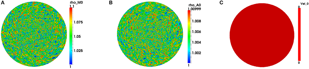
Figure 1. Initial conditions for the variables. We begin simulations by considering initial concentrations of the variables, respectively, as random perturbations about (A) ρ_m = 1.0, (B) ρ_a = 1.0, and (C) stationary cell at initial time. Blue signifies lowest values while red highest values.

We observe that the initial conditions chosen determine the dynamics of F-actin and cell shape. Choosing a perturbation about ρ_a = 1.0 as the initial condition for ρ_a variable leads to a uniform expansion of the cell. Figure 2 shows one set of solution set with initial data for the concentrations as random perturbation about ρ_m = 1 and ρ_a = 1 and all other parameters as in Table 2. In Figure 2C, we observe that the solution β^h has its highest value around the points where x² + y² = 0.8. These correspond to the points where δ(l) is discontinuous. Figure 2D shows change in area with time of the evolving cell. We varied the initial condition for ρ_a variable. Choosing a non-zero concentrations of ρ_a = 1.0 only in one half of the cell leads to symmetry breaking where the cell identifies its front and rear. This leads to an irregular expansion of the cell and hence in a directed migration of the cell toward the direction with high F-actin concentrations. Figures 3A–E is a solution set when considering initial data for myosin II as random perturbation about ρ_m = 1, initial condition for ρ_a non-zero only in one half of the cell and all other parameters as in Table 2. Figures 3E,F show the initial mesh and mesh at the end of the simulation, respectively.

FIGURE 2

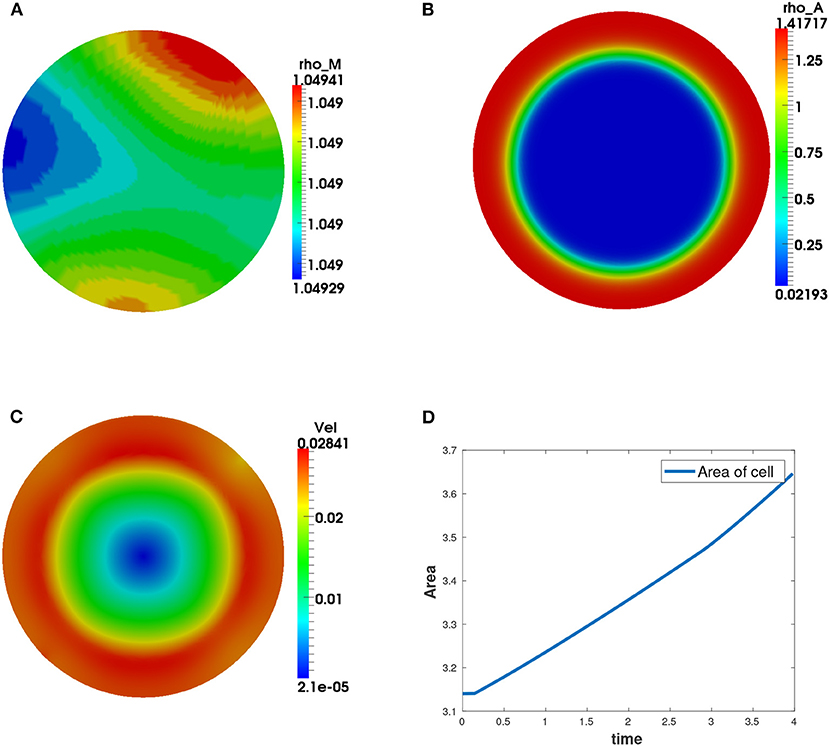
Figure 2. Graphical display of numerical solution illustrating a growing cell at time t = 4. This is a case when considering initial condition as random perturbations about ρ_a = ρ_m = 1.0. Blue signifies lowest values while red signifies highest values. (A) solution for ρ_m variable, (B) solution for ρ_a variable, (C) cell speed at final time showing higher speeds as the concentration of F-actin increases, and (D) area of the growing cell as a function of time showing increase in area of the cell with time.

FIGURE 3

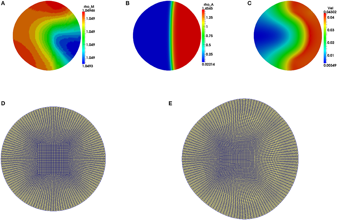
Figure 3. Graphical display of numerical solution illustrating a migrating cell at time t = 4 when considering a non-zero initial condition of ρ_a = 1 only in one half of the cell. Blue signifies lowest values while red signifies highest values. (A) Solution for ρ_m variable, (B) solution for ρ_a variable and (C) cell speed at final time. Polymerization of actin leads to cell deformation where the cell expands more in the regions with higher actin filament concentrations. (D,E) are the finite element meshes of the simulations at initial and final times, respectively, which have been enlarged for clarity.

Actin changes from its active state (F-actin) to inactive state (G-actin) and vice-versa through polymerization and depolymerization processes and hence the total amount of actin is conserved at all time as shown in Figure 4A. F-actin assembles together causing expansive stress on the cell. We varied the parameter for total amount of actin, ${\rho }_a^{tot}$, in the cell by considering three cases: ${\rho }_a^{tot}=10$, increasing the parameter to ${\rho }_a^{tot}=16$ and decreasing the parameter to ${\rho }_a^{tot}=5$. We observed that the more the total amount of actin, the more the expansion of the cell. Figures 4B–D show change in the area of the evolving cell with time as a result of varying the parameter ${\rho }_a^{tot}$. In our model, myosin II only diffuses inside the cell and therefore no reaction kinetics involving myosin II variable.

FIGURE 4

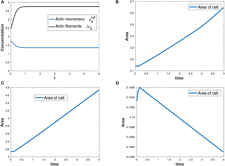
Figure 4. (A) Conservation of mass for actin with total amount of actin as ${\rho }_a^{tot}=10$, (B) area of the growing cell as a function of time for the case ${\rho }_a^{tot}=10$ as shown in Table 2, (C) area of the cell with an increased total amount of actin ${\rho }_a^{tot}=16$ while all other parameters in Table 2 held constant and (D) decreasing area of the cell with a reduced total amount of actin ${\rho }_a^{tot}=5$ while all other parameters in Table 2 held constant.

5. Conclusion and Future Directions

In this work, we considered an alternative approach to classical phase-fields approach by formulating the model equations on a sharp interface moving boundary problem for a single cell migrating on a two-dimensional moving domain. The problem involves a system of reaction-diffusion equations posed on a growing domain, where the velocity of the moving actin filaments is identical to the flow velocity of the domain and this velocity is modeled by a momentum balance equation within a viscous framework. In this approach the flow of the actin network is treated as a Newtonian fluid. We then employed the evolving finite element method to provide numerical approximate solutions of the model equations on the physical Lagrangian moving domain. This method does not allow for topological changes in cell shape unlike the phase-field model and also does not require a sufficiently refined mesh close to the sharp moving boundary interface. Furthermore, the method renders itself naturally to three-dimensional extensions.

Actin filaments and myosin II are the main sources of stresses in the cell and are responsible for driving cell migration. We varied the parameter for total actin and observed a linear relationship between the cell expansion and total amount of actin. The more the total amount of actin, the more the expansion. A decrease in the total amount of actin beyond a certain threshold leads to cell shrinking. Myosin II is responsible for cell contraction. By varying the contraction coefficient for myosin II, we observed contraction of the cell. The initial condition also played a role in the dynamics of cell migration. We considered two sets of initial conditions for the F-actin and myosin II variables. A random perturbation about ρ_a = 1 led to uniform expansion of the cell where the periphery of the cell expanded or contracted uniformly. By considering a non-zero initial concentration of F-actin only in one half of the cell, we observed a directed growth of the cell where the cell expanded in the direction with more actin concentration and began to migrate in that direction. The findings and conclusion from our work is therefore as follows: in the absence of advection of actin and myosin II and domain evolution, the biochemical model for F-actin and myosin II will reach steady state and that the actomyosin system is responsible for driving cell migration. Some of the parameters and variables that are important in the dynamics of cell migration are: the initial conditions for F-actin, the total amount of actin inside the cell, the contraction and polymerization coefficients.

In this paper, no rigorous numerical convergent analysis has been undertaken due to the complex nature of the coupling between mechanics and biochemistry during domain growth and this aspect forms part of our current studies. Furthermore, extensions of this work include the introduction of a mechanism for volume constraint or conservation, incorporation of cell adhesion and membrane forces, cell-to-cell interactions, extensions to many cells, cell migration through obstacles and formulating experimentally driven actomyosin reaction dynamics, just to mention a few.

Data Availability Statement

All datasets generated for this study are included in the article.

Author Contributions

All authors listed have made a substantial, direct and intellectual contribution to the work, and approved it for publication.

Funding

This work (AM) was partly supported by the EPSRC grant number EP/J016780/1, the European Union Horizon 2020 research and innovation programme under the Marie Sklodowska-Curie grant agreement no. 642866, the Commission for Developing Countries, and the Simons Foundation. AM is a Royal Society Wolfson Research Merit Award Holder funded generously by the Wolfson Foundation. AM is also a Distinguished Visiting Scholar to the University of Johannesburg, Department of Mathematics, South Africa. This work (BK) was carried out when BK was a graduate researcher at University of Sussex supported by University of Sussex Chancellor's International Research Scholarship.

Conflict of Interest

The authors declare that the research was conducted in the absence of any commercial or financial relationships that could be construed as a potential conflict of interest.

References

1. Ananthakrishnan R, Ehrlicher A. The forces behind cell movement. Int J Biol Sci. (2007) 3:303–17. doi: 10.7150/ijbs.3.303

PubMed Abstract | CrossRef Full Text | Google Scholar

2. Fidler IJ. The pathogenesis of cancer metastasis: the ‘seed and soil’ hypothesis revisited. Nat Rev Cancer. (2003) 3:453. doi: 10.1038/nrc1098

PubMed Abstract | CrossRef Full Text | Google Scholar

3. Gupta V. Rupture of multiple receptor-ligand bonds: bimodal distribution of bond rupture force. Eur Phys J E. (2012) 35:1–8. doi: 10.1140/epje/i2012-12094-9

PubMed Abstract | CrossRef Full Text | Google Scholar

4. Mogilner A. Mathematics of cell motility: have we got its number? J Math Biol. (2009) 58:105. doi: 10.1007/s00285-008-0182-2

PubMed Abstract | CrossRef Full Text | Google Scholar

5. Ridley AJ. Life at the leading edge. Cell. (2011) 145:1012–022. doi: 10.1016/j.cell.2011.06.010

PubMed Abstract | CrossRef Full Text | Google Scholar

6. Schwarz US, Safran SA. Physics of adherent cells. Rev Modern Phys. (2013) 85:1327. doi: 10.1103/RevModPhys.85.1327

PubMed Abstract | CrossRef Full Text | Google Scholar

7. Pollard TD, Borisy GG. Cellular motility driven by assembly and disassembly of actin filaments. Cell. (2003) 112:453–465. doi: 10.1016/S0092-8674(03)00120-X

PubMed Abstract | CrossRef Full Text | Google Scholar

8. Pollard TD. Regulation of actin filament assembly by Arp2/3 complex and formins. Annu Rev Biophys Biomol Struct. (2007) 36:451–77. doi: 10.1146/annurev.biophys.35.040405.101936

PubMed Abstract | CrossRef Full Text | Google Scholar

9. Pellegrin S, Mellor H. Actin stress fibres. J Cell Sci. (2007) 120:3491–9. doi: 10.1242/jcs.018473

PubMed Abstract | CrossRef Full Text | Google Scholar

10. Pollard TD, Blanchoin L, Mullins RD. Molecular mechanisms controlling actin filament dynamics in nonmuscle cells. Annu Rev Biophys Biomol Struct. (2000) 29:545–76. doi: 10.1146/annurev.biophys.29.1.545

PubMed Abstract | CrossRef Full Text | Google Scholar

11. Anderson KI, Cross R. Contact dynamics during keratocyte motility. Curr Biol. (2000) 10:253–60. doi: 10.1016/S0960-9822(00)00357-2

PubMed Abstract | CrossRef Full Text | Google Scholar

12. Zhu C, Bao G, Wang N. Cell mechanics: mechanical response, cell adhesion, and molecular deformation. Annu Rev Biomed Eng. (2000) 2:189–226. doi: 10.1146/annurev.bioeng.2.1.189

PubMed Abstract | CrossRef Full Text | Google Scholar

13. Cavalcanti-Adam EA, Volberg T, Micoulet A, Kessler H, Geiger B, Spatz JP. Cell spreading and focal adhesion dynamics are regulated by spacing of integrin ligands. Biophys J. (2007) 92:2964–74. doi: 10.1529/biophysj.106.089730

PubMed Abstract | CrossRef Full Text | Google Scholar

14. Cuvelier D, Théry M, Chu YS, Dufour S, Thiéry JP, Bornens M, et al. The universal dynamics of cell spreading. Curr Biol. (2007) 17:694–9. doi: 10.1016/j.cub.2007.02.058

PubMed Abstract | CrossRef Full Text | Google Scholar

15. Shemesh T, Bershadsky AD, Kozlov MM. Physical model for self-organization of actin cytoskeleton and adhesion complexes at the cell front. Biophys J. (2012) 102:1746–56. doi: 10.1016/j.bpj.2012.03.006

PubMed Abstract | CrossRef Full Text | Google Scholar

16. Burridge K, Wittchen ES. The tension mounts: stress fibers as force-generating mechanotransducers. J Cell Biol. (2013) 200:9–19. doi: 10.1083/jcb.201210090

PubMed Abstract | CrossRef Full Text | Google Scholar

17. Barry NP, Bretscher MS. Dictyostelium amoebae and neutrophils can swim. Proc Natl. Acad Sci USA. (2010) 107:11376–80. doi: 10.1073/pnas.1006327107

PubMed Abstract | CrossRef Full Text | Google Scholar

18. Campbell EJ, Bagchi P. A computational model of amoeboid cell swimming. Phys Fluids. (2017) 29:101902. doi: 10.1063/1.4990543

CrossRef Full Text | Google Scholar

19. Van Haastert PJ. Amoeboid cells use protrusions for walking, gliding and swimming. PLoS ONE. (2011) 6:e27532. doi: 10.1371/journal.pone.0027532

PubMed Abstract | CrossRef Full Text | Google Scholar

20. Campbell EJ, Bagchi P. A computational model of amoeboid cell motility in the presence of obstacles. Soft Matter. (2018) 14:5741–63. doi: 10.1039/C8SM00457A

PubMed Abstract | CrossRef Full Text | Google Scholar

21. Pullarkat PA, Fernández PA, Ott A. Rheological properties of the eukaryotic cell cytoskeleton. Phys Rep. (2007) 449:29–53. doi: 10.1016/j.physrep.2007.03.002

CrossRef Full Text | Google Scholar

22. Peskin CS, Odell GM, Oster GF. Cellular motions and thermal fluctuations: the Brownian ratchet. Biophys J. (1993) 65:316–24. doi: 10.1016/S0006-3495(93)81035-X

PubMed Abstract | CrossRef Full Text | Google Scholar

23. Mogilner A, Oster G. Cell motility driven by actin polymerization. Biophys J. (1996) 71:3030–45. doi: 10.1016/S0006-3495(96)79496-1

PubMed Abstract | CrossRef Full Text | Google Scholar

24. Mogilner A, Oster G. Force generation by actin polymerization II: the elastic ratchet and tethered filaments. Biophys J. (2003) 84:1591–605. doi: 10.1016/S0006-3495(03)74969-8

PubMed Abstract | CrossRef Full Text | Google Scholar

25. Marée AF, Jilkine A, Dawes A, Grieneisen VA, Edelstein-Keshet L. Polarization and movement of keratocytes: a multiscale modelling approach. Bull. Math. Biol. (2006) 68:1169–211. doi: 10.1007/s11538-006-9131-7

PubMed Abstract | CrossRef Full Text | Google Scholar

26. Satyanarayana S, Baumgaertner A. Shape and motility of a model cell: a computational study. J. Chem. Phys. (2004) 121:4255–65. doi: 10.1063/1.1778151

PubMed Abstract | CrossRef Full Text | Google Scholar

27. Satulovsky J, Lui R, Wang YL. Exploring the control circuit of cell migration by mathematical modeling. Biophys J. (2008) 94:3671–83. doi: 10.1529/biophysj.107.117002

PubMed Abstract | CrossRef Full Text | Google Scholar

28. Mogilner A, Edelstein-Keshet L. Regulation of actin dynamics in rapidly moving cells: a quantitative analysis. Biophys J. (2002) 83:1237–58. doi: 10.1016/S0006-3495(02)73897-6

PubMed Abstract | CrossRef Full Text | Google Scholar

29. Alt W, Dembo M. Cytoplasm dynamics and cell motion: two-phase flow models. Math Biosci. (1999) 156:207–28. doi: 10.1016/S0025-5564(98)10067-6

PubMed Abstract | CrossRef Full Text | Google Scholar

30. Gracheva ME, Othmer HG. A continuum model of motility in ameboid cells. Bull. Math. Biol. (2004) 66:167–93. doi: 10.1016/j.bulm.2003.08.007

PubMed Abstract | CrossRef Full Text | Google Scholar

31. Mogilner A, Marland E, Bottino D. A minimal model of locomotion applied to the steady gliding movement of fish keratocyte cells. In: Maini PK, and Othmer HG, editor. Mathematical Models for Biological Pattern Formation. New York, NY: Springer (2001). p. 269–93. doi: 10.1007/978-1-4613-0133-2_12

CrossRef Full Text | Google Scholar

32. Rubinstein B, Jacobson K, Mogilner A. Multiscale two-dimensional modeling of a motile simple-shaped cell. Multiscale Model Simul. (2005) 3:413–39. doi: 10.1137/04060370X

PubMed Abstract | CrossRef Full Text | Google Scholar

33. Stephanou A, Chaplain M, Tracqui P. A mathematical model for the dynamics of large membrane deformations of isolated fibroblasts. Bull Math Biol. (2004) 66:1119. doi: 10.1016/j.bulm.2003.11.004

PubMed Abstract | CrossRef Full Text | Google Scholar

34. George UZ. A numerical approach to studying cell dynamics (2012). PhD thesis, University of Sussex.

PubMed Abstract | Google Scholar

35. Biben T, Misbah C. Tumbling of vesicles under shear flow within an advected-field approach. Phys Rev E. (2003) 67:031908. doi: 10.1103/PhysRevE.67.031908

PubMed Abstract | CrossRef Full Text | Google Scholar

36. Biben T, Kassner K, Misbah C. Phase-field approach to three-dimensional vesicle dynamics. Phys Rev E. (2005) 72:041921. doi: 10.1103/PhysRevE.72.041921

PubMed Abstract | CrossRef Full Text | Google Scholar

37. Liu P, Zhang Y, Cheng Q, Lu C. Simulations of the spreading of a vesicle on a substrate surface mediated by receptor-ligand binding. J Mech Phys Solids. (2007) 55:1166–81. doi: 10.1016/j.jmps.2006.12.001

CrossRef Full Text | Google Scholar

38. Zhang J, Das S, Du Q. A phase field model for vesicle-substrate adhesion. J Comput Phys. (2009) 228:7837–49. doi: 10.1016/j.jcp.2009.07.027

CrossRef Full Text | Google Scholar

39. Lowengrub JS, Rätz A, Voigt A. Phase-field modeling of the dynamics of multicomponent vesicles: Spinodal decomposition, coarsening, budding, and fission. Phys Rev E. (2009) 79:031926. doi: 10.1103/PhysRevE.79.031926

PubMed Abstract | CrossRef Full Text | Google Scholar

40. Shao D. Computational Models on Cell Migration. PhD thesis. UC San Diego (2011).

Google Scholar

41. Shao D, Levine H, Rappel WJ. Coupling actin flow, adhesion, and morphology in a computational cell motility model. Proc Natl Acad Sci USA. (2012) 109:6851–6856. doi: 10.1073/pnas.1203252109

PubMed Abstract | CrossRef Full Text | Google Scholar

42. Camley BA, Zhao Y, Li B, Levine H, Rappel WJ. Crawling and turning in a minimal reaction-diffusion cell motility model: coupling cell shape and biochemistry. Phys Rev E. (2017) 95:012401. doi: 10.1103/PhysRevE.95.012401

PubMed Abstract | CrossRef Full Text | Google Scholar

43. Moure A, Gomez H. Phase-field modeling of individual and collective cell migration. Arch Comput Methods Eng. (2019). doi: 10.1007/s11831-019-09377-1. [Epub ahead of print].

CrossRef Full Text | Google Scholar

44. Shao D, Rappel WJ, Levine H. Computational model for cell morphodynamics. Phys Rev Lett. (2010) 105:108104. doi: 10.1103/PhysRevLett.105.108104

PubMed Abstract | CrossRef Full Text | Google Scholar

45. Elliott CM, Stinner B, Venkataraman C. Modelling cell motility and chemotaxis with evolving surface finite elements. J R Soc Interface. (2012) 9:3027–44. doi: 10.1098/rsif.2012.0276

PubMed Abstract | CrossRef Full Text | Google Scholar

46. Moure A, Gomez H. Phase-field model of cellular migration: three-dimensional simulations in fibrous networks. Comput Methods Appl Mech Eng. (2017) 320:162–97. doi: 10.1016/j.cma.2017.03.025

CrossRef Full Text | Google Scholar

47. Vanderlei B, Feng JJ, Edelstein-Keshet L. A computational model of cell polarization and motility coupling mechanics and biochemistry. Multiscale Model Simul. (2011) 9:1420–43. doi: 10.1137/100815335

PubMed Abstract | CrossRef Full Text | Google Scholar

48. Bottino DC, Fauci LJ. A computational model of ameboid deformation and locomotion. Eur Biophys J. (1998) 27:532–9. doi: 10.1007/s002490050163

PubMed Abstract | CrossRef Full Text | Google Scholar

49. Farutin A, Rafaï S, Dysthe DK, Duperray A, Peyla P, Misbah C. Amoeboid swimming: a generic self-propulsion of cells in fluids by means of membrane deformations. Phys Rev Lett. (2013) 111:228102. doi: 10.1103/PhysRevLett.111.228102

PubMed Abstract | CrossRef Full Text | Google Scholar

50. Najem S, Grant M. Phase-field approach to chemotactic driving of neutrophil morphodynamics. Phys Rev E. (2013) 88:034702. doi: 10.1103/PhysRevE.88.034702

PubMed Abstract | CrossRef Full Text | Google Scholar

51. MacDonald G, Mackenzie JA, Nolan M, Insall R. A computational method for the coupled solution of reaction-diffusion equations on evolving domains and manifolds: application to a model of cell migration and chemotaxis. J Comput Phys. (2016) 309:207–6. doi: 10.1016/j.jcp.2015.12.038

PubMed Abstract | CrossRef Full Text | Google Scholar

52. Ölz D, Schmeiser C. How do cells move? Mathematical Modeling of Cytoskeleton Dynamics and Cell Migration. Cell Mechanics: From Single Scale-Based Models to Multiscale Modelling. Boca Raton: Chapman and Hall/CRC (2010). doi: 10.1201/9781420094558-c5

CrossRef Full Text | Google Scholar

53. Manhart A, Oelz D, Schmeiser C, Sfakianakis N. An extended Filament Based Lamellipodium Model produces various moving cell shapes in the presence of chemotactic signals. J Theor Biol. (2015) 382:244–58. doi: 10.1016/j.jtbi.2015.06.044

PubMed Abstract | CrossRef Full Text | Google Scholar

54. Hirsch S, Manhart A, Schmeiser C. Mathematical modeling of Myosin induced bistability of Lamellipodial fragments. J Math Biol. (2017) 74:1–22. doi: 10.1007/s00285-016-1008-2

PubMed Abstract | CrossRef Full Text | Google Scholar

55. Mackenzie JA, Rowlatt CF, Insall RH. A conservative finite element ALE scheme for mass-conserving reaction-diffusion equations on evolving two-dimensional domains. (2019). arXiv[Preprint]. arXiv:191002282.

Google Scholar

56. Cusseddu D, Edelstein-Keshet L, Mackenzie JA, Portet S, Madzvamuse A. A coupled bulk-surface model for cell polarisation. J Theor Biol. (2019) 481:119–35. doi: 10.1016/j.jtbi.2018.09.008

PubMed Abstract | CrossRef Full Text | Google Scholar

57. Moure A, Gomez H. Three-dimensional simulation of obstacle-mediated chemotaxis. Biomech Model Mechanobiol. (2018) 17:1243–68. doi: 10.1007/s10237-018-1023-x

PubMed Abstract | CrossRef Full Text | Google Scholar

58. Moure A, Gomez H. Dual role of the nucleus in cell migration on planar substrates. Biomech Model Mechanobiol. (2020). doi: 10.1007/s10237-019-01283-6. [Epub ahead of print].

PubMed Abstract | CrossRef Full Text | Google Scholar

59. Morton KW, Mayers DF. Numerical Solution of Partial Differential Equations: An Introduction. Cambridge: Cambridge University Press (2005). doi: 10.1017/CBO9780511812248

CrossRef Full Text | Google Scholar

60. Mitchell AR, Griffiths DF. The Finite Difference Method in Partial Differential Equations. Chichester; New York, NY: John Wiley (1980).

Google Scholar

61. Süli E. Finite Element Methods for Partial Differential Equations. Oxford: Oxford University Computing Laboratory (2002).

Google Scholar

62. Reddy JN. An Introduction to the Finite Element Method. Vol. 27. New York, NY: McGraw-Hill (1993).

Google Scholar

63. Houston P, Schwab C, Süli E. Discontinuous hp-finite element methods for advection-diffusion-reaction problems. SIAM J Num Anal. (2002) 39:2133–63. doi: 10.1137/S0036142900374111

CrossRef Full Text | Google Scholar

64. Brebbia CA. The Boundary Element Method for Engineers. London: Pentech Press (1980). doi: 10.1007/978-3-662-11270-0

CrossRef Full Text | Google Scholar

65. Beskok A, Warburton TC. An unstructured hp finite-element scheme for fluid flow and heat transfer in moving domains. J Comput Phys. (2001) 174:492–509. doi: 10.1006/jcph.2001.6885

CrossRef Full Text | Google Scholar

66. Masud A, Hughes TJ. A space-time Galerkin/least-squares finite element formulation of the Navier-Stokes equations for moving domain problems. Comput Methods Appl Mech Eng. (1997) 146:91–126. doi: 10.1016/S0045-7825(96)01222-4

CrossRef Full Text | Google Scholar

67. Madzvamuse A, Wathen AJ, Maini PK. A moving grid finite element method applied to a model biological pattern generator. J Comput Phys. (2003) 190:478–500. doi: 10.1016/S0021-9991(03)00294-8

CrossRef Full Text | Google Scholar

68. Madzvamuse A, Maini PK, Wathen AJ. A moving grid finite element method for the simulation of pattern generation by Turing models on growing domains. J Sci Comput. (2005) 24:247–62. doi: 10.1007/s10915-004-4617-7

CrossRef Full Text | Google Scholar

69. Madzvamuse A. Time-stepping schemes for moving grid finite elements applied to reaction-diffusion systems on fixed and growing domains. J Comput Phys. (2006) 214:239–63. doi: 10.1016/j.jcp.2005.09.012

CrossRef Full Text | Google Scholar

70. Manhart A, Oelz D, Schmeiser C, Sfakianakis N. Numerical treatment of the filament-based lamellipodium model (FBLM). In: Graw F, Pahle J, Matthaus F, editors. Modeling Cellular Systems Cham: Springer (2017).

Google Scholar

71. Murphy L, Madzvamuse A. A moving grid finite element method applied to a mechanobiochemical model for 3D cell migration. (2019). arXiv[Preprint].arXiv:190309535.

Google Scholar

72. Madzvamuse A, George UZ. The moving grid finite element method applied to cell movement and deformation. Finite Elem Anal Design. (2013) 74:76–92. doi: 10.1016/j.finel.2013.06.002

CrossRef Full Text | Google Scholar

73. Madzvamuse A, Chung AH. Fully implicit time-stepping schemes and non-linear solvers for systems of reaction-diffusion equations. Appl Math Comput. (2014) 244:361–74. doi: 10.1016/j.amc.2014.07.004

CrossRef Full Text | Google Scholar

74. Ruuth SJ. Implicit-explicit methods for reaction-diffusion problems in pattern formation. J Math Biol. (1995) 34:148–76. doi: 10.1007/BF00178771

CrossRef Full Text | Google Scholar

75. Camley BA, Zhao Y, Li B, Levine H, Rappel WJ. Periodic migration in a physical model of cells on micropatterns. Phys Rev Lett. (2013) 111:158102. doi: 10.1103/PhysRevLett.111.158102

PubMed Abstract | CrossRef Full Text | Google Scholar

76. Yang FW, Venkataraman C, Styles V, Madzvamuse A. A robust and efficient adaptive multigrid solver for the optimal control of phase field formulations of geometric evolution laws. Commun Comput Phys. (2017) 21:65–92. doi: 10.4208/cicp.240715.080716a

CrossRef Full Text | Google Scholar

77. Lewis M, Murray J. Analysis of stable two-dimensional patterns in contractile cytogel. J Nonlinear Sci. (1991) 1:289–311. doi: 10.1007/BF01238816

CrossRef Full Text | Google Scholar

78. Rubinstein B, Fournier MF, Jacobson K, Verkhovsky AB, Mogilner A. Actin-myosin viscoelastic flow in the keratocyte lamellipod. Biophys J. (2009) 97:1853–63. doi: 10.1016/j.bpj.2009.07.020

PubMed Abstract | CrossRef Full Text | Google Scholar

79. Mori Y, Jilkine A, Edelstein-Keshet L. Wave-pinning and cell polarity from a bistable reaction-diffusion system. Biophys J. (2008) 94:3684–3697. doi: 10.1529/biophysj.107.120824

PubMed Abstract | CrossRef Full Text | Google Scholar

80. Kiplangat BK. Modelling and Simulations of a Viscous Model for Cell Migration. PhD thesis, University of Sussex (2019).

Google Scholar

81. Gilbarg D, Trudinger NS. Elliptic Partial Differential Equations of Second Order. Berlin; Heidelberg; New York, NY: Springer (2015).

Google Scholar

82. Larsson S, Thomée V. Partial Differential Equations with Numerical Methods. Berlin; Heidelberg: Springer (2003).

Google Scholar

83. Acheson DJ. Elementary Fluid Dynamics. Oxford: Oxford University Press (1990).

Google Scholar

84. Dziuk G, Elliott CM. Finite elements on evolving surfaces. IMA J Num Anal. (2007) 27:262–92. doi: 10.1093/imanum/drl023

CrossRef Full Text | Google Scholar

85. Bangerth W, Hartmann R, Kanschat G. deal.II-a general-purpose object-oriented finite element library. ACM Trans Math Softw. (2007) 33:24. doi: 10.1145/1268776.1268779

CrossRef Full Text | Google Scholar

86. Barrett R, Berry MW, Chan TF, Demmel J, Donato J, Dongarra J, et al. Templates for the Solution of Linear Systems: Building Blocks for Iterative Methods. Vol. 43. Philadelphia, PA: SIAM (1994) doi: 10.1137/1.9781611971538

CrossRef Full Text | Google Scholar

87. Freund RW, Golub GH, Nachtigal NM. Iterative solution of linear systems. Acta Num. (1992) 1:57–100. doi: 10.1017/S0962492900002245

CrossRef Full Text | Google Scholar

88. Saad Y. Iterative Methods for Sparse Linear Systems. Vol. 82. Philadelphia, PA: SIAM (2003) doi: 10.1137/1.9780898718003

CrossRef Full Text | Google Scholar