Topological Data Analysis of Vascular Disease: A Theoretical Framework

1. Introduction

Vascular disease is the primary cause of human mortality in the United States and worldwide^1,2. Accurate diagnosis for the prediction and treatment of vascular disease is crucial. Increasing the diagnosis success rate even by a few percent would result in saving a significant number of human lives. For this reason, a great deal of manpower and funding are used up for vascular research each year worldwide. Developing high precision diagnosis methodology is crucial for proper medial treatment and saving human lives. In this paper, we propose a new method of diagnosis using topological data analysis (TDA).

TDA has been proven to provide a new perspective and a new analysis tool in data analysis, inspiring researchers in various applications [1–3]. The analysis with TDA is based on persistent homology driven by the given topological space. Various forms of data from various applications are actively being used by researchers via TDA for possibly finding new knowledge out of the given data such as those in computational biology [4–8]. The work described in this paper is motivated by the clinical problem of the diagnosis of vascular disease. In this paper we explored how TDA could be used to understand the complexity of vascular flows, and proposed a theoretical framework of the new method that could characterize and classify the vascular flow conditions.

1.1. Existing Methodologies

1.1.1. Anatomical Approach

The most intuitive diagnosis method is the geometric approach. This approach is easy to practice and minimally invasive. As an anatomical approach, in angioplasty and stenting, the interventional cardiologist usually acquires multiple angiographic sequences, in an attempt to have one or more with the vessel in a minimally foreshortened presentation with minimal overlap. The interventional cardiologist then attempts to determine the extent of the disease involvement, using percent stenosis and length of the stenotic region from these angiograms. The degree of deformation is measured by the percent stenosis. The established estimates are frequently made by naked eyes, with potential errors being introduced, e.g., incorrect lengths due to foreshortening of the vessel, sizing errors due to improper estimates, improper calibration of the vessel magnification and/or inaccurate estimates of the extent of the plaque. These errors result in stents being incorrectly sized and/or too short, such that additional stents are required increasing cost, procedure time, and risk to the patient [9].

1.1.2. Functional Approach

Hemodynamics analysis and functional measurements combined as a functional approach, though, yield a better approach than the angiographic analysis. In the assessment and treatment of vascular disease, interventional clinicians evaluate the status of a patient vascular system via an angiography, intravascular ultrasound and, more recently, flow wires. While vessel geometry relates to functional status [10], flow rates are more closely related to the functional significance of the vascular abnormality [11]. For this reason, a flow wire has been widely used to assess the functional significance of a stenosis via the fractional flow reserve (FFR) [12–15]. Functional measurements of FFR using a flow wire yield a direct evaluation of the pressure gradient, providing a way of clinical judgment with accuracy. Despite the extra cost and risk [16, 17], the FFR combined with the angiography serves as a more accurate functional index for the pre-intervention than the geometric factors determined by the angiography alone.

The FFR is defined as the ratio of the maximum attainable flow in the presence of a stenosis to the normal maximum flow, which is uniquely given by the measure of the pressure gradient around the single lesion. The FFR as a functional index is then defined by the ratio of the proximal pressure to the distal pressure at maximum coronary vasodilation:

$\begin{array}{ll}FFR=\frac{P_p-P_v}{P_d-P_v},& (1)\end{array}$

where P_p, P_d, P_v are the proximal, distal and vasodilation pressures, respectively. In most cases, P_v is not elevated and considered P_v ~ 0. Thus, the FFR becomes $FFR=\frac{P_p}{P_d}.$

The FFR analysis of today is based on the following assumptions: (1) the pressures P_p and P_d used for the evaluation of the FFR are evaluated simultaneously by the flow wire, (2) the obtained FFR value represents the functional index for a single stenosis, and (3) the interaction of the flow wire device with the local flow movements is negligible in the measurements of P_p and P_d. The clinical norm with the FFR is roughly as follows: FFR <~ 0.75(0.8) implies that the lesion is functionally significant requiring intervention and FFR ≥~ 0.85(0.9) implies that the lesion is functionally not significant. Measurement of the FFR is not required for a stenosis of emergent severity (> 70% stenosis). However, for the lesion of intermediate severity the FFR plays a critical role because the geometry of the stenosis alone does not deliver enough information of the functional significance. The main advantage of using the FFR is its ability to measure the pressure gradient inside the stenotic region directly. Despite such an advantage, it requires additional costs and risk because it is more invasive. Furthermore, the functional analysis using FFR does not fully utilize the functional information of vascular flows because it measures the pressure drop only throughout the stenotic vessel. For this reason not every value of FFR provides a direct interpretation of the vasculature. Alternatively there have been investigations that use computational fluid dynamics (CFD) solutions to measure the FFR using the patient-specific CFD solutions [18] (also see recent reviews [19, 20]). Even with this approach, the FFR is only derived while other functional variables computed by CFD are not used. Thus, the CFD approach also has the same degree of ambiguity in interpreting the obtained value of FFR. We briefly mention that there are also various in vivo approach to the problem such as the recent experimental model [21].

1.2. Proposed Method

The anatomical analysis and the functional analysis yet may carry debatable diagnosis results for some vascular situations, particularly for the intermediate situations. Thus, more refined analysis is still demanded that could deliver more functional measures, and predict the future development of stenosis. The ideal method is to use the complete knowledge of all the hemodynamic variables. However, it is not even possible to relate every variable into a single numeric measure. Our primary approach to this problem is to attempt to use the relatively recent concept of TDA based on persistent homology. In this paper we explore the applications of persistent homology to the problem of stenotic blood vessels based on the preliminary work of Nicponski [22]. We first apply 1-dimensional persistent homology to a geometric model of a stenosed vessel's boundary, the vascular wall, to estimate the stenosed radius of the vessel using what we call the critical failure value of the vessel. We show that this critical failure has a close relationship with the disease level of the vessel. While the homology of a topological space is unaffected by how the space is stretched and deformed, we see that the persistent homology captures size information about an underlying space, as well as homology data. We then use velocity data projected onto the unit 2-dimensional sphere, S². The velocity data was generated by the 3D CFD using the spectral method. This approach is based on the 2-dimensional persistent homology. We show numerically that this spherical projection yields different topological properties for differing levels of stenosis. In our preliminary research, we found that it is possible to reveal the topological difference between the two vasculatures, and that the difference can be measured in a single numeric index through TDA. This new functional analysis for the stenotic vascular flows will significantly improve the existing analysis. Here we mention that the proposed method is highly related to the machine learning approaches that are recently investigated [23–25]. TDA analysis of vascular disease should be considered as a feature training in the context of machine learning, which will be investigated in our future research.

2. Simplicial Homology

In this section, we briefly explain simplicial homology and refer readers to [1, 26, 27] for more details. To understand persistent homology we must understand homology. In this paper we will be mainly concerned with the simplicial homology of a simplicial complex. This concept of a simplicial complex is fundamentally tied to the concept of persistent homology and thus we must first understand what a simplicial complex is.

2.1. Simplicial Complexes

Definition 2.1. A Simplicial Complex is a set of simplices S such that:

1. If s is an element of S, then all faces of s are also in S.

2. If s₁ and s₂ are in S, then s₁ ⋂ s₂ is either the empty set or a face of both.

Speaking informally, a simplicial complex is topological space made of vertices (0-simplex), edges (1-simplex), triangles (2-simplex), tetrahedrons (3-simplex), and higher dimensional equivalents attached to one another by their edges, vertices, faces, and so on. Generally speaking, simplicial complexes are a tool for building simple topologies. As we shall see later, a simplicial complex is simple enough that certain important topological features can be calculated numerically, namely the homology.

2.2. Simplicial Homology

The basic idea of homology is that homology describes the holes in a topological space. We shall see this clearly after we give a precise definition.

Definition 2.2. Let S be a simplicial complex, k, N ≥ 0 be integers and R be a ring with unit. A simplicial k-chain is a formal sum

${\displaystyle \sum _{i=1}^N}{c}_i{s}_i,$

where the c_i are elements of R and the s_i are k-simplices of S.

When referring to a simplex, one specifies the simplex and an orientation of that simplex. This is done by specifying the vertices and an ordering of those vertices. Permuting the vertices represents the same simplex multiplied by the sign of that permutation.

Definition 2.3. The free R-module C_k(S, R) is the set of all k-chains.

For technical reasons, we take C₋₁(S, R) to be the trivial module. We will write C_k(S, R) as simply C_k for this paper out of convenience. There is a natural map between these R-modules called the boundary map. Speaking imprecisely, the boundary map takes a simplex to its boundary. The precise definition follows:

Definition 2.4. The boundary map

${\delta }_k:C_k\to C_{k-1}$

is the homomorphism defined by

$\delta (v_0,\dots ,v_k)={\displaystyle \sum _{i=0}^k}{(-1)}^i(v_0,\dots ,v_{i-1},v_{i+1},\dots ,v_k).$

We take δ₀ to be the trivial map. It is not difficult to verify that δ_k−1 ○ δ_k = 0 for all k. Therefore, the kernel of δ_k−1 contains the image of δ_k. This leads to the definition of homology.

Definition 2.5. The kth homology module H_k(S, R) with coefficients in R is ker(δ_k)/Im(δ_k+1) [28].

While it is true that H_k is a module, we will simply refer to them as groups for convenience. As an example, let us take the simplicial complex X with the vertices labeled from left to right v₁, v₂, and v₃. We shall take our ring R to be the rational numbers, ℚ. The module C₀ is the set:

$C_0=\{a{v}_1+b{v}_2+c{v}_3|a,b,c\in \mathbb{Q}\}.$

For C₁ we must choose an orientation for our edges and will therefore orient them according to the index of their vertices. Thus, we have that C₁ is given by

$C_1=\{a(v_1,v_2)+b(v_1,v_3)+c(v_2,v_3)|a,b,c\in \mathbb{Q}\}.$

We have no higher dimensional simplices and thus C_k = 0 for k ≥ 2. The boundary map δ_k is necessarily the zero map for k ≠ 1. The boundary map δ₁ is defined by

${\delta }_1(v_i,v_j)=v_j-v_i,1\le i<j\le 3.$

Thus, we have that

$\begin{array}{l}{H}_0=C_0/<v_2-v_1,v_3-v_1,v_3-v_2>\\ \cong \{a{v}_1+b{v}_2+c{v}_3|a,b,c\in \mathbb{Q}\}/<v_j-v_i>.\end{array}$

Here the symbol < > means the vector space spanned by inside elements with ℚ. Simple algebra reveals that

$H_0=\{(a+b+c)v_1|a,b,c\in \mathbb{Q}\}\cong \mathbb{Q}.$

It is easy to see that the kernel of δ₁ is the submodule generated by (v₁, v₂) − (v₁, v₃) + (v₂, v₃) and the image of δ₂ is trivial. Thus,

$H_1=<a((v_1,v_2)-(v_1,v_3)+(v_2,v_3))|a\in \mathbb{Q}>\cong \mathbb{Q}.$

Finally it is easy to see that all other homology modules are trivial.

We need to understand what homology represents. As mentioned earlier, the homology groups represent holes. If our ring R is not a field, then the homology groups may have torsion. In this work, we will always calculate homology relative to a field, namely the rational numbers, ℚ. Therefore, the homology groups will be isomorphic to the product of some number of copies of R.

Let us determine the homology of the complex shown in the left of Figure 1 with coefficients in ℚ. The zeroth dimensional homology group describes the number of connected components. In the figure, we have two; the top component and the bottom component. Each connected component gives the zeroth homology a copy of the ring R, in our case, ℚ. Thus, H₀(X, ℚ) = ℚ². The first dimensional homology group describes the number of one dimensional holes, i.e., holes like the center of a circle. This figure has three. Each hole will give the homology group a copy of our ring R. Thus, H₁(X, ℚ) = ℚ³. There are no higher dimensional simplices and thus the higher homology groups are trivial. If we fill in one of the holes with a triangle shown in the right of Figure 1, then we now have only two holes. This new space, Y, has H₁(Y, ℚ) = ℚ². We can also think of the first dimensional homology as representing the number of loops that can be drawn in the topological space that cannot be pulled closed. The torus has two. Thus, the first homology group of the torus would be ℚ². The second dimensional homology group describes the number of two dimensional holes, i.e., holes like the interior of a sphere. Each hollow of a topological space gives the second homology group a copy of our ring R. This torus has one hollow, thus its second homology group is ℚ. In general, the nth homology group measures n dimensional holes, i.e., holes similar to the interior of the n dimensional sphere. In this work we will not go higher than second dimensional homology because our analysis in this paper does not require higher dimensions.

FIGURE 1

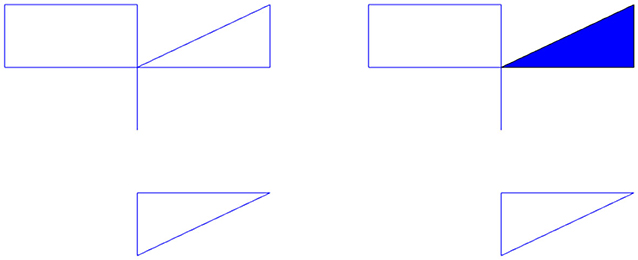
Figure 1. (Left) Example topological space, X. (Right) The space X with a hole filled in is the space Y.

Definition 2.6. The kth Betti number for a topological space X, β_k, is the rank of the kth homology group.

As we have seen above, for each n dimensional topological space there is a copy of the ring R in our homology group. The Betti numbers therefore represent the number of holes in each dimension.

3. Persistent Homology

The primary topological feature we explore is that of persistent homology [1]. We will first give a brief overview of this concept. Given some point data, called a point cloud, that are points on some surface or other manifold, we generate a complex that is hopefully a reasonable approximation of the original manifold. Given the points, we will assign edges and triangles (and higher order simplices) to pairs, triples, etc. of the point cloud. Roughly speaking, if a pair of points are close to each other, we add an edge between them and similarly for faces. To assign edges and higher order simplices, we introduce a parameter t, called the filtration value. This t is the length of the largest edge that may be included in our simplex. We will let t vary and at each value we will create the complex, calculating the homology of the complex at each t value.

There are, generally, at least three strategies to make use of this parameter to assign simplices. The Vietoris-Rips strategy [29] places an edge between two points if their distance is less than t and a face between three points if their pairwise distance is less than t, and so on. This strategy is fine, but computationally expensive. The next strategy is the witness strategy [30] which takes two subsets of the points, called landmark points and witness points. The landmark points serve as vertices of our complex. We will place an edge between two landmark points if there is a witness point within distance t of both points, a face if there is a witness point within t of all three points, and so on. Usually all of the points in the point cloud are used as witnesses. The last strategy is the lazy-witness strategy [30], where edges are assigned identically to the witness strategy, however faces and higher simplices are assigned anywhere there are n points that are all pairwise connected with edges. We will be using the lazy-witness streams for our computation due to the reduced complexity of the calculation. It is also worth noting that in the witness and lazy witness methods, there is sometimes an extra mechanism used to help decrease noise. For this mechanism, rather than compare distances to t, we compare distances to t + η_n(p) where η_n(p) is the distance from p to its nth nearest neighbor and p is the witness point being considered. This tends to remove some noise for low t values.

Let us see an example. Consider the following point cloud (the left figure of Figure 2): Let us construct the Vietoris complex for this point cloud at various values of t. At time t = 0 there are no edges to add (the left figure of Figure 2). We see the same point cloud at t = 0.25 (the right figure of Figure 2). It is important to understand that although the points all lie on a plane, the edges and triangles should be considered to pass through higher dimensions so as to not intersect, except at their common faces. In this figure, we have added arrows to indicate the five obvious holes that are present. It is conceivable that there may be more holes hidden, but we will see that this is not the case. In Figure 3, we see that the point cloud now is topologically the same as an annulus, with only the middle hole present. It is also worth observing that as t increases, the central hole is gradually becoming smaller and will eventually be closed with a large enough value of t.

FIGURE 2

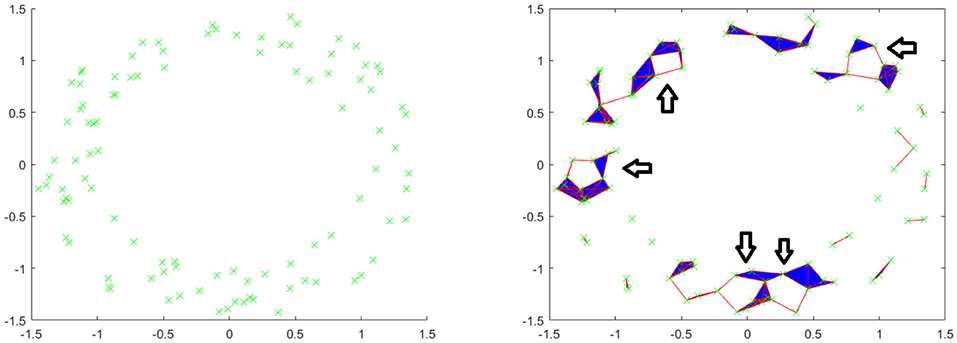
Figure 2. (Left) Example point cloud with 100 points. (Right) Vietoris complex at t = 0.25. Five arrows are included to point out five holes.

FIGURE 3

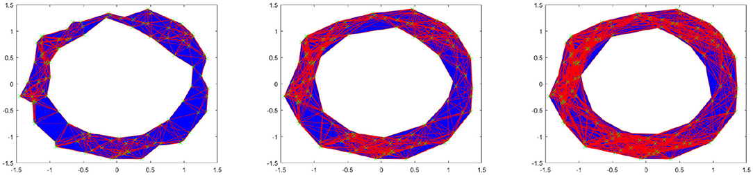
Figure 3. Vietoris complex at t = 0.5, 0.75, 1 from left to right.

Of interest to us in the context of persistent homology are the Betti numbers. We saw previously that the zeroth Betti number is the number of connected components, the first is the number of one dimensional holes, the second is the number of two dimensional holes, and so on. Because we are looking at homology relative to this parameter t, we have Betti numbers for each individual value of t. Thus, instead of simple Betti numbers, we will have Betti intervals. The graphs of these intervals will make up what is called a barcode. For these calculations, we have used the Javaplex software package from [31].

The left figure of Figure 4 shows the barcode by the Vietoris-Rips method. In the figure, the horizontal axis is the filtration value t. Vertically we have multiple stacked intervals graphed that correspond to individual generators of the homology groups. In the zeroth dimension we see many generators that correspond to many disconnected components when t is small, which eventually are connected into a single component when t is larger. In the first dimension we see a number of small circles that are quickly closed up and one circle that lasts a long time corresponding to the one large hole in the center of the annulus. We have placed rectangles about the five intervals that are present at t = 0.25 that correspond to the five holes seen in the right figure of Figure 2. We have only generated barcodes for the zeroth and first dimensions. It is conceivable that there may be interesting topology in higher dimensions, but because this example is meant to illustrate, we see no reason to include the higher dimensions. While there may be higher dimensional homology occurring, such homology would only be noise, because we have started with a two dimensional topological space.

FIGURE 4

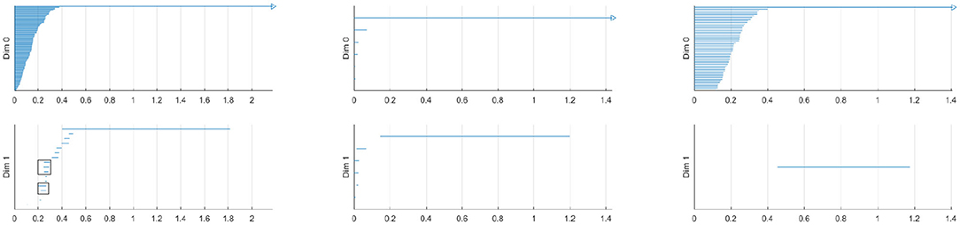
Figure 4. (Left) Barcode for point cloud using Vietoris-Rips method. The five intervals in dimension one present at t = 0.25 are boxed. (Middle) Barcode for point cloud using witness method with 50 landmark points. (Right) Barcode for point cloud using lazy witness method with 50 landmark points.

Comparing this barcode to our Figures 2, 3, we can see how the barcode compares with our intuition. At t = 0, we had no edges and only vertices, thus we had many different connected components. We can count the Betti numbers at a particular time t from the barcode by counting the number of intervals that overlap that value of t. Because the zeroth dimension corresponds to connected components, if we look at t = 0 in the dimension zero portion of the barcode we see many intervals, one for each point. At t = 0.25, we saw about 17 connected components and about 5 holes. If we look at our barcode at t = 0.25, in the first dimension we see about 5 intervals and in the zeroth dimension we see about 17. For t = 0.5 and greater, we saw only the center of the annulus for a hole and only one connected component. If we look at the barcode at these t values, we see only one interval in both the first and second dimensions. Finally, note that at about t = 1.8, the last interval in the first dimension is gone. This represents the center of the annulus being filled up and thus there are no more one dimensional holes.

The middle and right figures of Figure 4 show the barcode by the witness and lazy witness methods, respectively. Because there is a choice inherent in the witness and lazy witness methods, choosing the landmark points, these are not unique. Performing these calculations a second time will generate a different barcode. It is also worth pointing out that if an interval is shorter than the minimum t step, then those intervals are not shown. In the middle figure, we have several connected components at t = 0, which quickly become a single connected component at approximately t = 0.1. We also see a number of one dimensional holes when t is small, but by t = 0.2 there is exactly one hole left, the annulus center. In the right figure, we see a number of intervals in the zeroth dimension, but again we see that eventually we only have one connected component. In the first dimension we only see one hole, which lasts for a wide interval. This again corresponds to the central hole of the annulus.

All of these barcodes give essentially the same information. The individual points are quickly connected and we eventually have a single connected component. There are some small circles that quickly disappear and we are quickly left with one persistent circle which lasts for a while and then is filled.

3.1. Calculating Persistent Homology

The complete algorithm for calculating persistent homology can be found in [3]. We will briefly summarize the algorithm here. To compute the homology of a simplicial complex, one must understand the boundary operator δ. Since we are looking at homology relative to a field, the chain groups and homology groups, C_k and H_k, are vector spaces. Therefore, one can consider δ_k to a linear map between vector spaces. Because we are interested in homology, we are interested in the kernel of this map, as well as the image. We may use the standard basis of the chain groups, specifically the k-chains, as our basis. Let us use as an example the complex in Figure 5. The basis for C₀ is {a, b, c, d} and the basis for C₁ is {bc, cd}. Here we are referring to the edges by their endpoints. If we write the standard matrix for δ₀, it would simply be the zero matrix. If we write the matrix for δ₁, relative to the bases in the order given above, then we would get

$\begin{array}{l}{\delta }_1=\left(\begin{array}{cc}0& 0\\ 1& 0\\ -1& 1\\ 0& -1\end{array}\right).\end{array}$

To compute the kernel of our matrix, we will transform the matrix into Smith normal form. To do this, we use elementary row and column operations. Specifically, we may swap two columns, add a multiple of one column to another and multiply one column by a non zero constant. The row operations are similar. Each of these operations correspond to a change of basis in either C₁ or C₀. If we add row two to row three and then row three to row four, our new matrix will be

$\begin{array}{l}{\delta }_1=\left(\begin{array}{cc}0& 0\\ 1& 0\\ 0& 1\\ 0& 0\end{array}\right).\end{array}$

Our new basis for C₀ will be {a, b-c, c-d, d}. The basis for C₁ is unchanged because we used no column operations.

FIGURE 5

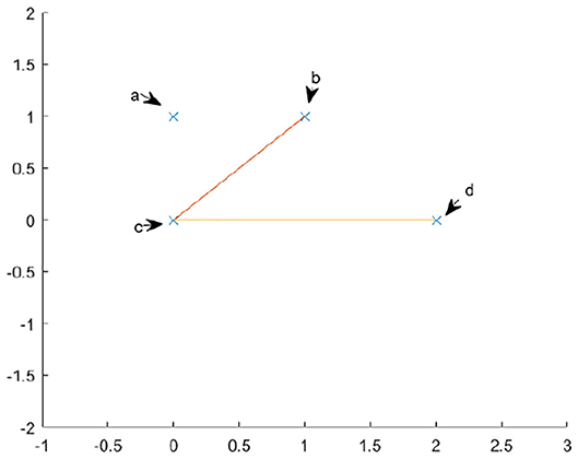
Figure 5. An example topological space.

From this calculation, we see that the map δ₁ has trivial kernel and a two dimensional image. The image is the subspace generated by {b−c, c−d}. Because the kernel of δ₀ is {a, b−c, c−d, d} and the image of δ₁ is {b−c, c−d}, we have that H₀ is just the vector space spanned by {a, d}. We know our H_n is a vector space, because we are calculating homology with coefficients over a field, thus the only important piece of information is the dimension. We can simply read off the dimension by looking at the number of pivot positions in δ₁ and the number of non pivot columns in δ₀. There are four non pivot columns in δ₀ and two pivot positions in δ₁, therefore the first homology group is $H_0\cong {\mathbb{Q}}^2$. Therefore, by simply transforming the matrix into Smith normal form, we may simply read off the dimensions of kernels and images of the δ_k and simply take their difference to find the dimensions of our homology group.

To calculate persistent homology is a harder task. For this we must have the definition of a persistence module. In our case, we will receive as input a number of complexes, all representing the same point cloud for different values of our filtration variable t. Let us call the chain complex at the kth timestep $C_n^k$. We will similarly call the kernels and boundary groups $Z_n^k$ and $B_n^k$, respectively. For each $C_n^k$, there is a natural inclusion map

$i:C_n^k\to C_n^{k+1}.$

Definition 3.1. The persistence module associated to $\{C_n^k\}$ is the R[t] module

${\displaystyle \underset{k=1}{\overset{\infty }{\oplus }}}{C}_n^k,$

where

$t(x_1,x_2,\dots )=(0,i(x_1),i(x_2),\dots ).$

Here, R is our field.

It is shown in the same paper that calculating the homology of this persistence module is equivalent to calculating the intervals that appear in the barcode. Due to the structure theorem [2], that every graded module M over a graded PID (principal ideal domain), R[t], decomposes uniquely into the form

$\left({\displaystyle \underset{i=1}{\overset{n}{\oplus }}}{\Sigma }^{{\alpha }_i}R\left[t\right]\right)\oplus \left({\displaystyle \underset{j=1}{\overset{m}{\oplus }}}{\Sigma }^{{\gamma }_j}R\left[t\right]/t^{n_j}\right),$

where Σ^α represents an upward shift in grading. Thus, our persistence modules $C_n^k$, will give rise to persistent homology groups $H_n^k$, which will decompose in the above manner.

It was shown in [2], that factors of the form ΣⁱR[t]/t^j−i correspond to persistent intervals of the form (i, j) in our barcode. Similarly, each free factor, ΣⁱR[t] corresponds to an interval of the form (i, ∞). Thus, the crux of the problem comes down to finding and decomposing the homology of our persistence modules. To accomplish this, we may simply use row and column reduction as in the example above. The finer details, along with some simplifications, are laid out in the original paper.

3.2. Persistence

One central idea of persistent homology is the concept of persistence. Referring to Figure 4, we had only one interval in the zeroth dimension that was rather long and many shorter intervals. Similarly, in the first dimension we again had one long interval and many shorter ones. By making use of our prior knowledge that the point cloud was coming from an annulus, we see that the “real" features, namely one connected component and one circle, correspond to the long intervals and the shorter intervals are noise. It is reasonable to assume that this holds frequently (though not certainly) in general data sets. Usually longer intervals will correspond to "real" features and shorter intervals correspond to noise. How one interprets what is “real" depends on one's a priori knowledge of the underlying data structure. This leads us readily to our next definition.

Definition 3.2. The persistence of an interval [a, b] is the length of the interval, b − a.

While we have not given any proof that longer intervals tend to be more important than shorter intervals, in [1], there is an argument given that solidifies this mindset. Speaking imprecisely, the various methods of building simplicial complexes out of point clouds fall inside a hierarchy under inclusion. The lower methods (lazy witness and witness) are easier to compute but less accurate. The higher methods (Vietoris-Rips and other methods not discussed in this paper) are more complex to calculate, but more accurate. If a barcode has an interval with sufficient length, then this guarantees a corresponding interval in the higher complexity methods. We refer the reader to [1, 26, 29] for more details.

For more details on computing persistent homology with matrix analysis, we refer readers to a recent review by Carlsson et al. [32].

4. Critical Failure Value

First we will use a simple model of a stenosed vessel to explore the topological structure of a vessel. We will initially only consider the exterior of a vessel, which topologically speaking is a cylinder. A stenosed blood vessel is characterized by a narrowing of that vessel. We shall consider the typical radius of our vessel to be r₀ = r_healthy and will assume that the stenosis takes the shape of a Gaussian distribution for simplicity. We will also assume a small amount of noise, in the form of a uniform random variable ϵ ∈ [0, 0.1]. We will take r_st to be the difference between the normal radius and the stenosed radius. Therefore, our model will be, in cylindrical coordinates

$r=r_0+ϵ(z,\theta )-r_{st}{e}^{-z^2},-a\le z\le a,0\le \theta \le 2\pi$

where the stenosis is at z = 0 and r₀ − r_st is the radius of the cylinder at the stenosis. Thus, r_st is a measure of how stenosed the vessel is, specifically the vessel has a stenosis percentage of $100\left(1-\frac{r_{st}}{r_0}\right).$ When working with real data we will not have any equation that represents the surface of the vessel, rather we will have point data approximating the surface. Therefore, for our model we will use some discrete points on the surface. To have an accurate picture, the number of points should be high. In the left figure of Figure 6 we have an example of the above model. The figure clearly shows the vessel narrowing near the origin, which is the stenosed portion of the vessel. The points are colored according to their y-coordinate to give depth.

FIGURE 6

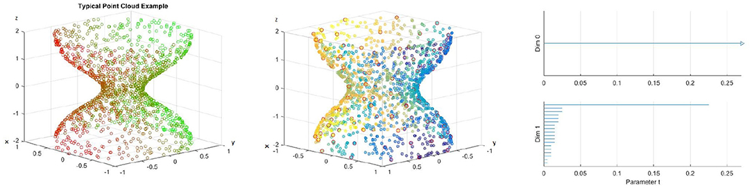
Figure 6. (Left) Example of a point cloud representing a 70% stenotic vessel. (Middle) A point cloud with landmark points highlighted in red. (Right) Barcode.

4.1. A First Example

For our first application example, we will use 1, 500 points for our blood vessel model above, with 100 landmark points. We use the lazy witness method described above. The points are selected randomly on our surface and the landmark points are selected using an algorithm that selects points uniformly according to pointwise distance. An image of the point cloud with the landmark points circled in red is included in the middle figure of Figure 6, and points are colored to give depth. We use the lazy witness strategy and get the barcode for those in the left and middle of Figure 6. As we saw above, each interval corresponds to a generator of homology in the corresponding dimension. We can see that the homology is for the most part the homology of a cylinder. Initially there is some noise when t is small, but until about t = 2.3 we have exactly one connected component and a single one dimensional hole. This t value where the last one dimensional generator becomes trivial is what we call the critical failure value below.

4.2. Critical Failure Value

We saw above that for large t values our complex no longer has any one dimensional holes. The exact value where this occurs will be of particular importance to us.

Definition 4.1. Let B be a barcode, with intervals {(a_i, b_i)} in the first dimension. We call the critical failure value (CFV) of B to be max(b_i).

This definition should be fairly straightforward. For example, in the right figure of Figure 6 the critical failure value would be the largest right endpoint of an interval in the first dimension. Thus, the critical failure value for that barcode would be CFV = 0.23. This critical failure value is of particular importance to us because we shall see that it approximates the stenosis of the vessel. The critical failure value is a generalization of percent stenosis. The exterior of the blood vessel is a cylinder. The ends of the cylinder are open and thus we have a one dimensional hole, the hollow center of the cylinder. If the ends were capped then we would have a two dimensional hole instead. We are using persistent homology and thus we are approximating the point cloud with simplicial complexes as described above. As t increases we add more and more edges and triangles to our complex. Eventually, as we saw in the annulus example above, we will have triangles that span the hollow of our cylinder. When this occurs, our simplicial complex no longer is a hollow cylinder and thus has different homology.

Definition 4.2. Suppose P is a point cloud with points chosen from the topological space S. The principal critical failure value of P is the critical failure value of S.

Speaking generally, suppose we have a point cloud of data that is contained in a 2D shape (or 3D solid, etc.) S with n points. We call this point cloud S_n. If n is very large, and the points are more or less evenly spread out, then it is reasonable to expect that CFV(S_n) ≈ CFV(S), assuming some reasonable conditions regarding S. In fact, it is reasonable to write that ${\text{lim}}_{n\to \infty }CFV(S_n)$ = CFV(S), again assuming some reasonable conditions about S and the method under which the points are chosen. The critical failure value and principal critical failure values will depend heavily on which method one uses to calculate the persistent homology. We will use subscripts to indicate which method is being referred to. We mentioned that when calculating persistent homology using the lazy witness method, sometimes one may choose to include the complexity of considering the nth nearest neighbor for points when constructing our simplexes. When one is constructing the persistent homology of a topological space, rather than a point cloud, there will not usually be an nth nearest neighbor, as any point will usually have infinitely many points arbitrarily near it. Thus, when constructing the persistent homology of such a set, we will not include the nearest neighbor complexity.

Theorem 1. For S a circle of radius R, CFV_w(S) = CFV_lw(S) = R. Here the subscripts w and lw denote the witness and lazy witness methods, respectively.

Proof: First, observe that in the zeroth and first dimensions, the complexes created using the witness and lazy witness methods are identical, and therefore the principal critical values for these two methods will be identical.

Let us consider a circle of radius R centered at the origin and an inscribed regular hexagon, as pictured in Figure 7A. The reader can verify that the distance between neighboring vertices of the hexagon is R. Let us suppose that our parameter τ = t < R. We will consider a two simplex on the circle that may be generated using the witness and lazy witness methods under this setup. We will show that such a simplex does not contain the center of the circle and therefore the first dimensional homology of our complex is nontrivial. This will imply that the critical failure value of our circle is greater than t.

FIGURE 7

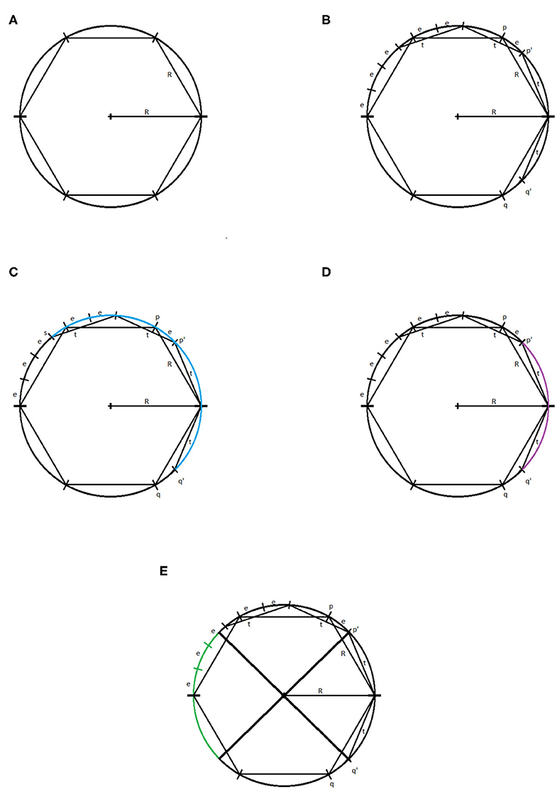
Figure 7. (A) Circle of radius R with inscribed hexagon. (B) The points p, q, p′, q′, and (R, 0). (C) The arc connecting the point s to the point q′ highlighted in blue. (D) The arc connecting the point p′ to the point q′ highlighted in purple. (E) The reflection of the arc connecting p′ and q′, in green.

Let p and q be the vertices of the inscribed hexagon adjacent to (R, 0). We suppose that we have a one simplex with vertices p′ and q′. We assume, without loss of generality, that the witness point for p′ and q′ is (R, 0). If not, we may rotate the circle until these two vertices straddle (R, 0) and then necessarily can take (R, 0) to be our witness. Because τ < R, it must be the case that p′ and q′ lie between p and (R, 0), and q and (R, 0), respectively. For the moment, we assume that the distance between p′ and (R, 0), and q′ and (R, 0) is exactly t, as pictured in Figure 7B.

We will label the distance between p and p′ as e > 0. Now, observe that, if one starts at the point (R, 0) and steps around the circle counterclockwise in steps of size R, one will reach the point (−R, 0) in exactly three steps. If one repeats this process but now stepping in steps of size t, one will not reach as far as the point (−R, 0) in three steps. Speaking precisely, one will be exactly three steps of length e away from the point (−R, 0), call this point s.

If one starts at the point p′ and steps clockwise about the circle twice in steps of length t, then one exactly reaches the point q′. We recall that any witness point connecting p′ to another point must be within t distance of p′, and any landmark point connected to p′ must be within t distance of that witness point. Thus, the set of points that may be connected to p′ to form a simplex under the witness and lazy witness methods is precisely the arc connecting the point s to the point q′ containing the point p′, as shown in Figure 7C.

Similarly, any point that may be connected to q′ to form a simplex would be contained in a similar arc around q′. Any point that may be connected to both p′ and q′ must be contained within both arcs. The intersection of these two arcs is precisely the arc from p′ to q′, as pictured in Figure 7D. However, any simplex with vertices p′, q′, and a third vertex within this arc does not contain the origin.

Now suppose that the points p′ and q′ have distance to (R, 0) less than t. Repeating the above construction, the arc that surrounds p′ of points that may be connected to p′ is simply rotated clockwise by the same amount that p′ has been rotated. Similarly the arc about q′ is rotated counterclockwise the same amount that q′ has been rotated. This rotation of these two arcs can widen their intersection, but still cannot generate a simplex containing the origin. To see that this is true, notice that for a simplex to contain the origin, the third vertex would need to be contained in the reflection of the arc connecting p′ and q′ across the origin on the other side of the circle, pictured in Figure 7E. While the arcs of points that may be connected to p′ and q′ may intersect this region, they do not intersect inside this region. Further, moving p′ and q′ closer to the point (R, 0) does not cause these two arcs to intersect within this region.

In any case, we have shown that if τ < R, then there is no one-simplex that contains the origin and therefore the homology in the first dimension of our complex contains at least one generator.

To see that the critical failure value is at most R, observe that if τ = R, then we may construct a simplex with landmark points and witness points at alternating vertices of the inscribed hexagon. This simplex includes the origin, and all other points can easily be covered. Thus, the critical failure value of a circle of radius R is R. □

Corollary 2. Let $S=\{(r\text{cos}(\theta ),r\text{sin}(\theta ),z),r=r_0-r_{st}{e}^{-z^2},-a\le z\le a\}$. Then CFV_w(S) = CFV_lw(S)= r₀ − r_st.

To prove this, we will need two brief lemmas.

Lemma 3. Let C₁ and C₂ be two circles centered at the origin, with the radius of C₁ = r₁ < r₂ = radius of C₂. Let p be the point (r₁, θ₁) and q be the point (r₂, θ₂) in polar coordinates. Also let q′ be the point (r₁, θ₂). Then the distance from p to q is greater than the distance from p to q′.

Proof: (Left figure of Figure 8) Let us calculate the distance between p and q using the law of cosines and the triangle with vertices at p, q, and the origin. By the law of cosines, if d₁ is the distance between p and q, then

$d_1^2=r_1^2+r_2^2-2r_1{r}_2\text{ cos}(\gamma )$

where γ is the angle ∠poq. If we rearrange slightly, we get

$d_1^2={(r_2-r_1)}^2+2r_1{r}_2(1-\text{cos}(\gamma )).$

If we replace r₂ with r₁, we get d₂, the distance between p and q′.

$d_2^2={(r_1-r_1)}^2+2r_1^2(1-\text{cos}(\gamma )).$

Observing that we have made one positive term zero and the second non-negative term becomes either strictly smaller or remains zero, thus we have the lemma proven. □

FIGURE 8

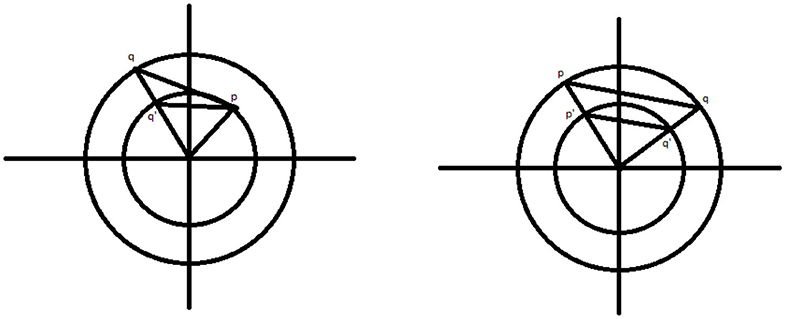
Figure 8. (Left) The points p, q, and q′. (Right) The points p, q, p′, and q′.

Lemma 4. Let C₁ and C₂ be two circles as above. Let p = (r₂, θ₁) and q = (r₂, θ₂). Also let p′ = (r₁, θ₁) and q′ = (r₁, θ₂). Then the distance between p and q is larger than the distance between p′ and q′.

Proof: (Right figure of Figure 8) Observe that the triangles △poq and △p′oq′ are similar and the result is clear. □

Proof of Corollary: To prove this, first observe that, due to Theorem 1, the circle at z = 0 is filled in exactly when τ = r₀ − r_st. Thus, the critical failure value of our set is at most r₀ − r_st. Next we show that our critical failure value is at least r₀ − r_st.

First, suppose that τ = t and that our first homology group is trivial. It must be the case that some simplex of our complex intersects the z axis. Let p_i = (r_i, θ_i, z_i), i = 1…6, be the landmark points and witness points of such a simplex. It is a relatively simple exercise to show that replacing these six points with $p_i^{\prime }$ = (r_i, θ_i, 0) does not increase any pairwise distance (though now these projections may not be contained within S). Further, observe that the simplex with vertices given by these projected vertices still intersects the z axis at the origin.

Next, notice that the closest our set S to the z axis is on the circle made up of the intersection of S with the plane z = 0. We will call this circle C. Observe that, we simply moved our original points vertically and therefore did not change their distance from the z axis. Thus, our projected points are at least as far from the z axis as the radius of C. Therefore, we see that r_i ≥ r₀ − r_st. Now, using our two lemmas repeatedly, we see that replacing our points $p_i^{\prime }$ with $p_i^{″}=(r_0-r_{st},{\theta }_i,0)$ does not increase any pairwise distance. Further, the new simplex still intersects the z axis. Thus, we see that these new points give us a simplex that fills in the center of C, with landmark and witness points given by the p_i”. By the theorem, it is not possible for such a simplex to exist if τ < r₀ − r_st, and therefore τ = t ≥ r₀ − r_st. □

The above corollary demonstrates that, without noise, if we have enough points on the surface of our model, we expect that the critical failure value will give us our stenosis radius almost exactly. To see empirically how well our estimate works with noise, we will generate a point cloud on our model of a stenotic vessel, with noise, and calculate the persistent homology as outlined above, many times. We will take r₀ = 1, and r_st a random variable taking values from [0, 1] and will plot the critical values against r_st. For this experiment, in each iteration, we use a total of 1, 500 randomly chosen points and 400 landmark points, approximately evenly spaced. We performed this experiment a total of 80 times. The results of the experiment are pictured in Figure 9.

FIGURE 9

Figure 9. Critical failure value against the stenosis radius r_st.

From Figure 9, we can see, as expected, that the relationship between the critical value and r₀ − r_st is approximately linear. There is some nonlinearity for large values of r_st. This is due to the minimal radius being approximately the same size as the noise, which is caused by gaps in the model due to too few points. Our expectation is that as the number of points and landmark points are increased the relationship between the critical value and r_st will be approximately

$\text{CFV}=1-r_{st}.$

This is due to our blood vessel having a normalized healthy radius of 1. For a general vessel, we expect the critical value to be approximately

$\text{CFV}=r_{healthy}-r_{st}.$

For different shapes of stenosis, we conjecture that this critical failure value would still be a measure of stenosis, though the exact relationship between stenosis and CFV would depend on the shape of the vessel.

We see from our above calculations that the critical failure value is related to the minimal radius of the vessel, thus giving us an idea of the stenosis of the vessel that is determined entirely by the point data of the vessel. This stenosis level can potentially be calculated directly from the vessel without the use of this critical failure value in some cases, and therefore the question of the usefulness of this critical failure value must be considered in our future work. The critical failure value will be defined for practically any shape of vessel, whether or not the stenosis is shaped like a Gaussian or any number of other symmetric or asymmetric shapes. Further, this critical value does not require exact knowledge of the location of the stenosis. In our model above, the stenosis was at z = 0, but if we instead had it at z = 1, or any other height, these calculations would generate the same results. This suggests that the critical value may be useful in automating the diagnosis of stenosis. We also expect that the critical value method may act as a sort of universal measurement for all different types of stenosis.

We have demonstrated that size data is encapsulated within the barcodes. Not only do the barcodes give the homology of a topological space, but also measurement data as well. It is therefore reasonable to suggest that in this problem as well as many others, reading off this size information may be critical. For example, we speculate that a similar method may be used to measure the widening of vessels, aneurysms.

If we replaced our model above with a model that had Gaussian widening instead of narrowing, thus modeling an aneurysm, then we would be interested in how wide the widest portion of the vessel is. This could potentially be estimated by looking for the largest t value where there is a second dimensional generator. To understand this geometrically, we realize that at a relatively small time step the two ends of the vessel will be capped off by triangles spanning their diameter, due to having a smaller radius than the aneurysm. When these ends are capped, we will have a large hollow, namely the interior of the vessel. This hollow will eventually be filled with tetrahedrons, and therefore become trivial. The t value where this happens will depend on how wide the vessel has become, and therefore that t value would be a measure of the wideness of the vessel.

Because the definition of persistent homology depends on the distances between points, the fact that persistent homology encapsulates not only homology information but size and diameter information is reasonable. Taking radius and size data from persistent homology can potentially have significant applications in many different real world problems, not just in the context of stenotic vessels.

5. 3D CFD and Spherical Projection

5.1. Hemodynamic Modeling

For modeling stenotic vascular flows, we use the incompressible Navier-Stokes equations with the no-slip boundary conditions at the blood vessel walls. A more precise description should consider the compressibility and more general types of boundary conditions such as Navier boundary conditions and boundary conditions based on the molecular model. However, as the main focus of this paper is on the global behavior of stenotic vascular flows, the incompressible Navier-Stokes equations with no-slip boundary conditions suffice to consider.

Let ρ = ρ(x, t) be the density, P = P(x, t) the pressure, u = (u, v, w)^T the velocity vector for the position vector x = (x, y, z)^T ∈ Ω, and time t ∈ ℝ⁺. Here Ω is the closed domain in ℝ³. We assume that the blood flow we consider is Newtonian. From the mass conservation we have the following equations

$\begin{array}{l}\rho {\text{u}}_t+(\text{u}·\nabla )\text{u}-\mu \nabla \text{u}-(3\lambda +\mu )\nabla (\nabla ·\text{u})+\nabla P=f\\ \begin{array}{l}{\rho }_t+\nabla ·(\rho \text{u})=0,\end{array}& (2)\end{array}$

where μ ∈ ℝ⁺ is the kinematic viscosity, λ ∈ ℝ is the bulk viscosity constant, and f is the external force. Further we assume that the density is homogeneous in x and t. Then the above equations are reduced to

$\begin{array}{l}\rho {\text{u}}_t+\rho \text{u}·\nabla \text{u}-\mu \nabla \text{u}+\nabla P=0\\ \begin{array}{l}\nabla ·\text{u}=0,\end{array}& (3)\end{array}$

where we also assume that there is no external force term f. For the actual numerical simulation we use the normalized equations. For example, the length scale is x_o = 0.26, the baseline velocity is u_o = 30, the time scale $t_o=6.7\times 10^{-3}$, the unit pressure P_o = 900, the unit density ρ_o = 1, and the unit kinematic viscosity μ = 0.0377 (all in cgs units) [33]. For the incompressible Navier-Stokes equations, we need to find the unknown pressure P. In this paper, we used the Chorin's method, i.e., the artificial compressibility method [34, 35]. For the Chorin's approach, we seek a steady-state solution at each time such that

${\text{u}}_t\to 0,P_t\to 0,t>t_s$

for ∇·u → 0. Then for the artificial compressibility, we introduce an auxiliary equation for p such that

$p_{\tau }+c\nabla ·\text{u}=0$

where τ is the pseudo-time. The pseudo-time is the time for which we solve the above equation for the given value of t until ∇·u → 0 at each t.

To solve the governing equations numerically, we adopt the spectral method based on the Chebyshev spectral method. We use N_t elements. Each element is a linear deformation of the unit cube, ${\Omega }_c={\left[-1,1\right]}^3$. We expand the solution in each domain as a Chebyshev polynomial of degree at most N. Let ξ be ξ ∈ [−1, 1] and T_l(ξ) be the Chebyshev polynomial of degree ℓ. Then in each element, the solution u is given by the tensor product of T_l(ξ).

To explain this further, we consider the 1D Chebyshev expansion. The 3D is simply a tensor product of the 1D expansion. The 1D Chebyshev expansion is given by

$u_N(\xi ,t)={\displaystyle \sum _{\ell =0}^N}{\widehat{u}}_{\ell }(t)T_{\ell }(\xi ),$

where $\widehat{u}$_ℓ are the expansion coefficients. Once the expansion coefficients are found, the solution is obtained as a linear combination of the Chebyshev polynomials with the expansion coefficients. For the spectral methods, we adopt the spectral collocation method so that the expansion coefficients are computed by the individual solutions at the collocation points. For the collocation points, we use the Gauss-Lobatto collocation points,

${\xi }_i=-\text{cos}(i\pi /N),i=0,1,\cdots ,N.$

We solve the incompressible Navier-Stokes equations on x(ξ_i) and the expansion coefficients are given by the quadrature rule based on the Gauss-Lobatto quadrature

${\widehat{u}}_{\ell }(t)=\frac{2}{c_{\ell }N}{\displaystyle \sum _{i=0}^N}\frac{1}{c_i}u(x({\xi }_i),t)T_{\ell }(x({\xi }_i)),$

where c_n = 2 if n = 0 and c_n = 1 otherwise [36].

The 3D Chebyshev approximation is given by a tensor product of the 1D Chebyshev expansion. Figure 10 shows some vessels we use for the numerical simulation. Figure 11 shows some spectral solutions of the stenotic vessel (left) and vessels with stent installed (right).

FIGURE 10

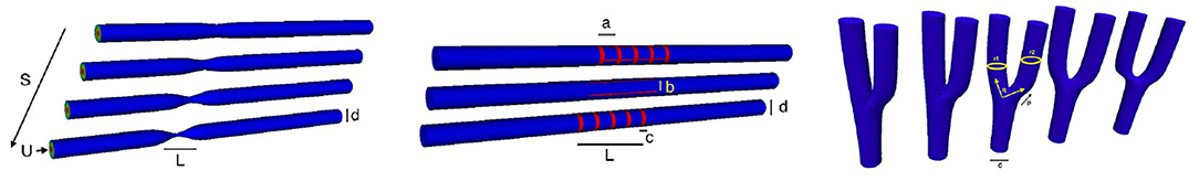
Figure 10. Parameterization: A simple illustration of variation of symmetric straight stenotic vessels (left) and the vessel configuration after the insertion of stent (middle) and variation of the bifurcating vessels (right).

FIGURE 11

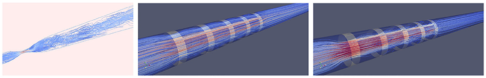
Figure 11. High-order spectral simulations of stenotic vessels. (Left) Stenotic vessel (70%). (Right) Numerical simulation with stent installed.

5.2. Spherical Projection

In this section we propose the spherical projection and TDA with the spherical projection based on the two dimensional homology. We will use vascular data calculated by solving the incompressible Navier-Stokes equations with the spectral method as outlined in section 5.1. Of particular interest to us are the velocity fields of blood flows in the vessel. When the vessel is healthy one has essentially laminar flow. When the vessel is diseased, we may see flow circulations. We first investigate the data in the phase space with the three velocity components.

In the left figure of Figure 12 the data is visualized in the phase space. The left figure shows the data for 10% stenosis and the right for 70%. Each axis is corresponding to each velocity component. The long axis is the y-axis, which is the flow direction. There is not a huge topological difference between those two stenosis, at least in terms of homology. There are no hollow portions or apparent significant circles that would give interesting homology. Thus, both would be topologically trivial.

FIGURE 12

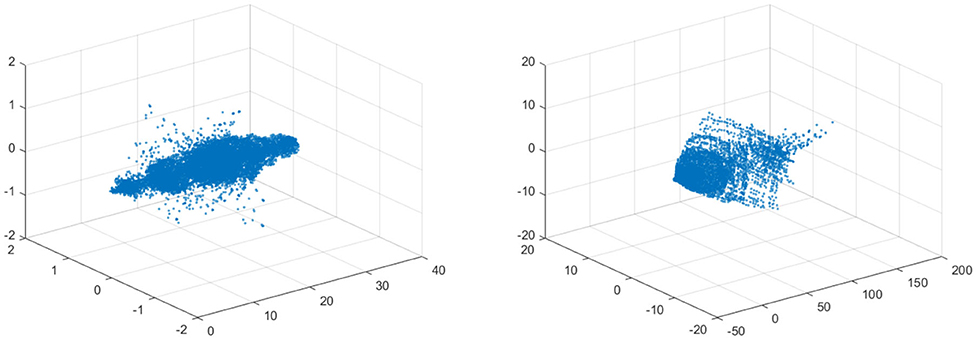
Figure 12. (Left) Velocity fields of 10% stenosis. Units are centimeters per second. (Right) Velocity fields of 70% stenosis. Units are centimeters per second.

To construct a meaningful topological space, we found that the projection of the raw data onto the n-unit sphere, which we call an n-spherical projection, is the key element of TDA of vascular disease [22]. To understand why the projection approach works, we consider the case of random fields where the 3D velocity and pressure are all randomly generated. The left figure of Figure 13 shows the spherical projection of the random velocity fields on S². The right figure of Figure 13 shows the spherical projection of the random velocity and pressure fields on S³. It is not plausible to visualize S³. Instead, in the right figure, the pressure contour is shown on top of velocity fields data. The color represents the pressure distribution. Notice that the sphere S² in the left figure is hollow but the sphere in the right is not. Figure 14 shows the corresponding barcodes to the spherical projection of the random velocity fields on S² (left) and the spherical projection of the random velocity and pressure fields on S³ (right). As shown in the figures, a hole appears at t ≈ 0.4 and disappears at t ≈ 0.9 in the second dimension (left figure for S²) and in the third dimension (right figure for S³). The interval where hole is existent in S² (left) and in S³ (right) in the barcodes is significant and it represents the underlying topology well. We define the persistence of an n-dimension interval, Π_n as

${\Pi }_n=b-a,$

where a is the value of t when the hole starts to appear and b is t when the hole disappears. In Figure 14, Π₂ ≈ 0.5 for the left figure and Π₃ ≈ 0.4 for the right. The parameter, Π_n serves as a measure of the complexity and we hypothesize that Π_n is directly related to the level of disease.

FIGURE 13

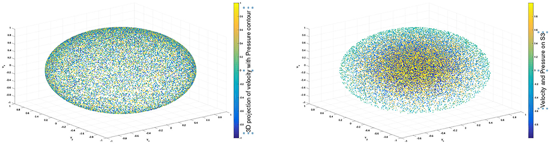
Figure 13. n spherical projection. (Left) Random velocity fields on S². (Right) Random velocity and pressure fields on S³.

FIGURE 14

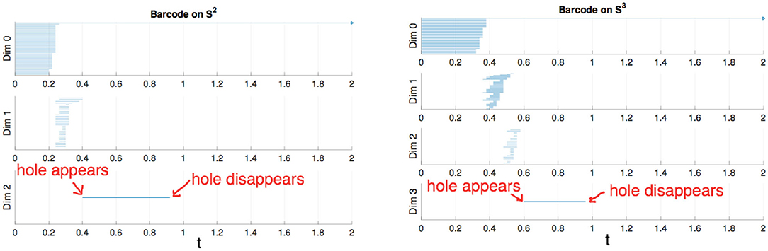
Figure 14. (Left) Barcode for data on S². (Right) Barcode for data on S³.

Definition 5.1. Fundamental projection: Let $\overrightarrow{v}$ = (v_x, v_y, v_z) be a non-zero velocity vector. We first normalize $\overrightarrow{v}$. The fundamental projection is the projection of the normalized velocity fields onto the unit sphere,

$<v_x,v_y,v_z>\to (v_x,v_y,v_z)/\Vert v\Vert ,$

where ‖v‖ is the norm of velocity fields, e.g., $\Vert v\Vert =\sqrt{v_x^2+v_y^2+v_z^2}$.

Definition 5.2. n-spherical projection: The n-spherical projection is the general projection that involves more variables, including the velocity fields, such as the pressure, P. If the pressure data is included, the spherical projection is done by

$<v_x,v_y,v_z,P>\to (v_x,v_y,v_z,P)/\sqrt{v_x^2+v_y^2+v_z^2+P^2}.$

The physical implication of the topological structure for the fundamental projection seems obvious but the one for the general projection n ≥ 3 is not, and we need to conduct a parameter study using the CFD solutions in order to understand its meaning in our future work.

For the projection, any zero vectors are removed prior to the projection. Note that all the velocity components on the vessel wall vanish due to the no slip boundary condition. The results of the fundamental projection of Figure 12 are shown in Figure 15 for 10% (left) and 70% (right) stenosis. We have colored the points according to their original norm, with red points having higher norm and blue points having lower norm, although the majority of points are blue and only a handful of points near the poles are red. The difference between the left and right figures in Figure 15 is clear—one is a sphere and the other is not. More precisely, the 70% stenosed projection has points all over the sphere, whereas the 10% stenosed projection only has points on the pole of the sphere. To see the topological difference between these two, we can use our tool of persistent homology. We expect the first to have no generators in the second dimension and the second to have one.

FIGURE 15

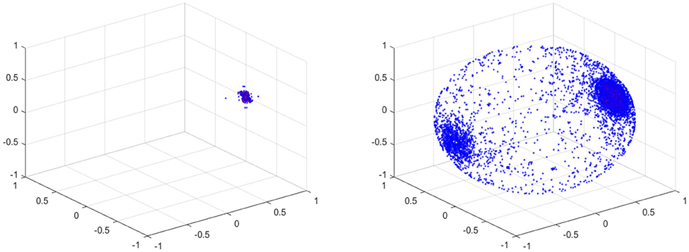
Figure 15. (Left) Spherical Projection of the normalized velocity fields of the Blood Vessel with 10% stenosis. (Right) Spherical Projection of the normalized velocity fields of the Blood Vessel with 70% stenosis.

It is worth observing that our vascular data is of the form $<\overrightarrow{s},\overrightarrow{U},P>$, with $\overrightarrow{s}$ being spatial data, $\overrightarrow{U}$ being velocity data, and P being scalar pressure data. The fundamental projection therefore reduces our topology from a seven dimensional space to a two dimensional space, namely the surface of the sphere. An advantage of this projection is that three dimensional data can be readily visualized—however, a lot of information may be lost in this reduction.

5.3. Persistent Homology of Spherical Projections

The process of the proposed method should be clear already; take the velocity data from a stenosed vessel and calculate its projection on the unit sphere, which we call its spherical projection (fundamental projection as we use the first three velocity components). Next we calculate its persistent homology. Since this calculation has high complexity, we use a fraction of our points as in the earlier calculations. We use the lazy witness strategy with 200 witness points and 150 landmark points. We make a choice of points when we perform our computation, and therefore there is a measure of imprecision inherent in our results. If we simply choose our points randomly, there is a chance that we will choose badly. If we wrongly chose a set of landmark points that were clustered together near a pole, we would make a poor deduction as to the coverage of the sphere. Because the sphere is a fixed scale, it does not take many points that are evenly spaced to properly cover the sphere. Therefore, if we make sure to choose our landmark points to be as evenly spaced as possible out of all possible choices, we can be confident that we avoid this case.

We have used the Javaplex package from [31] to calculate the barcodes. It is worth pointing out that when calculating the barcodes using Javaplex, if there are no intervals calculated above a certain dimension, then that dimension may not be graphed.

As we should suspect from the earlier Figure 15, the spherical projection for the vessel with 10% stenosis has no meaningful homology in the higher dimensions while 70% has clearly. Figure 16 shows the barcode of 10% stenosis (left) and 70% (right). As shown in the figure, we distinguish the healthy 10% stenosis from the diseased 70% stenosis in terms of topology, for which the spherical projection was crucial. In Appendix, we collect the spherical projection of velocity fields and its barcode for the cases of 20–60% stenosis. For all of these calculations we have used symmetric vascular data. By symmetric, we mean radial symmetry of the vessel. All the figures in Appendix show clearly how the spherical projections are effective and how the corresponding barcodes change as the degree of stenosis increases. As clearly shown in the figures, the persistence of the barcode in 2D becomes longer as disease develops. Table 1 shows the persistence vs. the amount of stenosis.

FIGURE 16

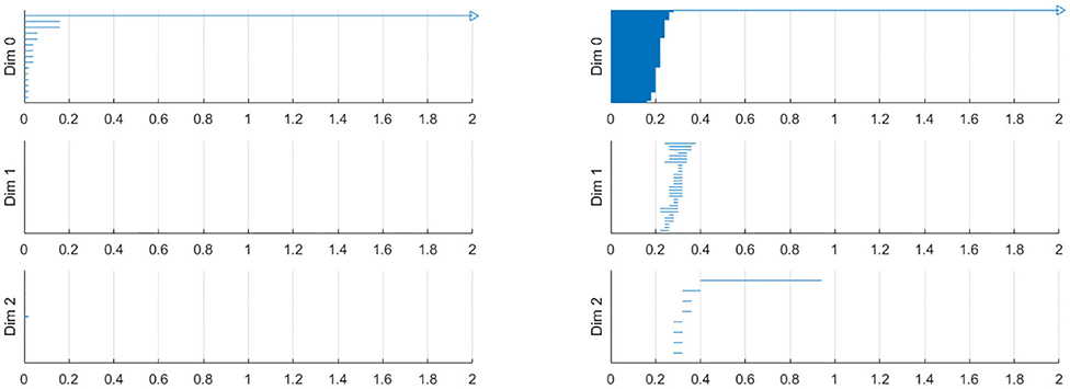
Figure 16. Barcodes of blood vessel with 10% stenosis (left) and 70% stenosis (right).

TABLE 1

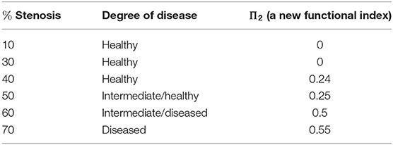
Table 1. Π vs. percent stenosis.

We also performed a similar calculation using asymmetric data for which the vessel will be stenosed different amounts in the two directions transverse to blood flows. For example, the first vessel is 40% stenosed in the one direction and 10% stenosed in the other direction in Figure 17. It is important to realize that an asymmetric vessel may have more circulation than a symmetric vessel and therefore even the less stenosed vessels will have circulation.

FIGURE 17

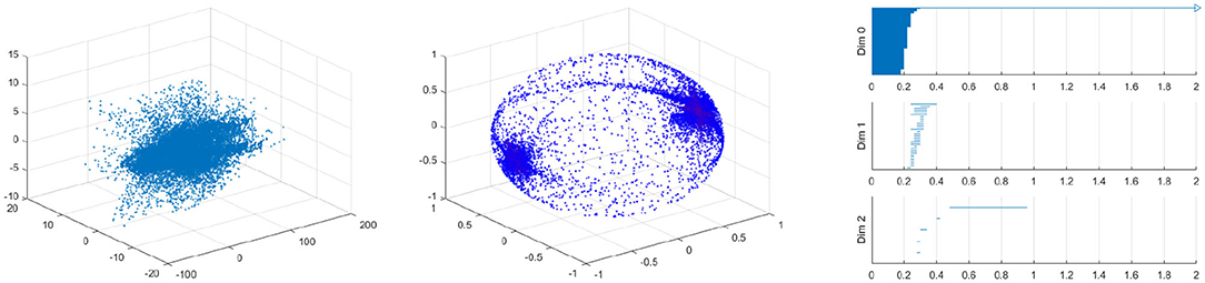
Figure 17. Velocity fields of vessel with 40% by 10% stenosis (left), the spherical projection (middle), and the corresponding barcode (right).

Figure 17 shows the raw data (left) and the spherical projection (middle) and the barcode for 40% by 10% asymmetric vessel. Here observe that the sphere is completely covered and there is an additional feature in the form of a ring about the equator. This ring was not present on the symmetric vessel cases and therefore immediately suggests that the spherical projection may be useful in differentiating between different types of stenosis. The right figure of Figure 17 shows the corresponding barcodes where we see a number of circles and one long persistence (two dimensional hole) of 2D persistent homology. In Appendix, we provide the results for 40 by 20%, 40 by 30%, 40 by 50%, 40 by 60% asymmetric stenosis. Another important feature that is in all of these asymmetrical vessels, as well as in the high stenosis symmetric vessels, is a clusters of points near the positive and negative y-direction poles. These represent the majority of blood flowing forward and a smaller but significant amount of blood flowing backward. As shown in [37], it is natural to develop asymmetry when the stenosis is being developed.

We have also performed this analysis for a vessel with a ring stent (Figures 18, 19). A ring stent that constitutes a series of parallel rings is implanted in the vessel to keep the vessel open (left figure in Figure 18). The right figure shows the barcode and Figure 19 shows the raw data (left) and the spherical projection (right). As shown in these, the flow circulation is captured in 2D barcode. We observe that there is much circulation in the vessel and therefore there is a two dimensional hole.

FIGURE 18

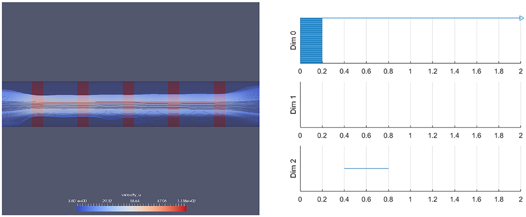
Figure 18. A blood vessel with a ring stent inserted (left) and the corresponding barcode (right).

FIGURE 19

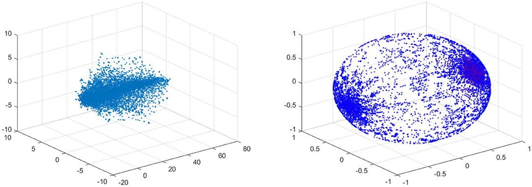
Figure 19. Velocity fields of ring stented vessel (left) and the spherical projection (right).

5.4. Higher Dimensional Spherical Projections

In the previous sections, we have focussed solely on velocity data. Velocity fields of vascular flows somewhat naturally map to the unit sphere precisely because circulation naturally corresponds to a spherical projection covering the unit sphere. However, there may be useful data to be extracted from projecting some or all of the higher dimensional data onto higher dimensional spheres, or even other topological spaces. This leads to the n-spherical projection of an n-dimensional non-zero vector (Definition 5.2).

How useful this idea of higher dimensional spherical projections remains to be investigated and will be considered in our future work. For example, one might consider the four dimensional projection of velocity and pressure data combined onto the three-sphere. There may be important information encoded here, but what that information is and how it is encoded are less clear, in part because this higher dimensional projection is much less natural than the fundamental projection. Perhaps a more natural alternative would be to project velocity and pressure data onto S² × I, where I is an interval. Pressure is a scalar in our data and certainly non-negative and therefore this projection may be more natural. Exploring the information present within these higher dimensional projections is a topic for a later paper; we merely include it here for completeness.

6. Concluding Remarks

In this paper, we proposed to use TDA of vascular flows. The key element of the proposed method is to use the patient-specific CFD data and apply TDA to obtain meaningful functional indices such as the critical failure value and the persistence of the vascular flows.

In this paper, first we explained the concepts of homology and persistent homology and gave examples of their use. We applied the concept of persistent homology to the geometry data of the exterior of the vessel thereby generating the so-called critical failure value. We demonstrated numerically that this critical failure value has a close relationship with the stenosis level of a vessel, and therefore may be used to measure stenosis. This method may be used for various vessel shapes, and may help serve as a general method of measuring stenosis. Further, this method demonstrates the potential application to determine size information about a topological object.

We next developed the concept of the spherical projection to understand and quantify vascular flows. We demonstrated that the spherical projection reveals important information and patterns about flow conditions that are not apparent to the naked eye. We applied the method to various data and demonstrated the differences thereof. This concept of spherical projection may be critical to understand and classify the different types and levels of stenosis. We applied the spherical projection method to different sets of vascular data, and showed clear differences between the barcodes for the different stenosis levels and types. The barcodes for the vessels with high stenosis were different compared to the less stenosed vessels. Additionally the asymmetric vessels were different from the symmetric vessels in their spherical projections, due to the presence of the equatorial ring.

The spherical projection may be generalized to data from higher dimensions. We have only used the velocity data for our calculations, while we have pressure data as well. Curvature may also be calculated from the vessel geometry, which could be another useful piece of data. Projecting some or all on a higher dimensional sphere and calculating the persistent homology should be considered in our future research. The spherical projection is naturally physical but simply projecting higher dimensional data onto a sphere may not be the best projection to consider. Rather, we conjecture that the particular projection should be targeted, based on intelligent analysis and understanding of the data in question.

In this paper, we focused on developing the theoretical framework of the proposed method. The data set of vascular flows has been obtained from the CFD calculations with simplified vessel configurations. To verify the applicability of the proposed methods, we have applied the proposed method to real patient data and obtained a promising preliminary data, which will be presented in our upcoming paper.

Data Availability Statement

All datasets generated for this study are included in the article and Appendix.

Author Contributions

JN and J-HJ developed the theoretical framework for the new diagnosis method of vascular disease. JN and J-HJ produced all numerical results using the 3D vascular flow profiles by the 3D spectral collocation code written by J-HJ. JN was a Ph.D. student and J-HJ supervised the project. This work was a part of JN's dissertation. All authors contributed to the article and approved the submitted version.

Funding

This research was partially supported by Samsung Science & Technology Foundation SSTF-BA1802-02 and also partially by Ajou University.

Conflict of Interest

The authors declare that the research was conducted in the absence of any commercial or financial relationships that could be construed as a potential conflict of interest.

Acknowledgments

The authors thank Kenneth Hoffmann for his valuable comments on their work. This manuscript has been released as a pre-print at: https://www.biorxiv.org/content/10.1101/637090v1 (JN and J-HJ).

Footnotes

1. ^http://www.heart.org/HEARTORG/

2. ^https://www.cdc.gov

References

1. Carlsson G. Topology and data. Bull Am Math Soc. (2009) 46:255–308. doi: 10.1090/S0273-0979-09-01249-X

CrossRef Full Text | Google Scholar

2. Zomorodian AJ. Topology for Computing. Cambridge Monographs on Applied and Computational Mathematics. Cambridge: Cambridge University Press (2005).

Google Scholar

3. Zomorodian A, Carlsson G. Computing persistent homology. In: SCG ‘04 Proceedings of the Twentieth Annual Symposium on Computational Geometry New York, NY (2004). p. 347–56.

Google Scholar

4. Cámara PG. Topological methods for genomics: present and future directions. Curr Opin Syst Biol. (2017) 1:95–101. doi: 10.1016/j.coisb.2016.12.007

PubMed Abstract | CrossRef Full Text | Google Scholar

5. Nicolau M, Levine AJ, Carlsson G. Topology based data analysis identifies a subgroup of breast cancers with a unique mutational profile and excellent survival. Proc Natl Acad Sci USA. (2011) 108:7265–70. doi: 10.1073/pnas.1102826108

PubMed Abstract | CrossRef Full Text | Google Scholar

6. Saggar M, Sporns O, Gonzalez-Castillo J, Bandettini PA, Carlsson G, Glover G, et al. Towards a new approach to reveal dynamical organization of the brain using topological data analysis. Nat Commun. (2018) 9:1399. doi: 10.1038/s41467-018-03664-4

PubMed Abstract | CrossRef Full Text | Google Scholar

7. Sauerwald N, Shen Y, Kingsford C. Topological data analysis reveals principles of chromosome structure throughout cellular differentiation. In: Huber KT, Gusfield D, editors. Leibniz International Proceedings in Informatics (LIPIcs), Vol. 143. Dagstuhl: Schloss Dagstuhl-Leibniz-Zentrum fuer Informatik (2019). p. 1–23. doi: 10.1101/540716

CrossRef Full Text | Google Scholar

8. Topaz CM, Ziegelmeier L, Halverson T. Topological data analysis of biological aggregation models. PLoS ONE. (2015) 10:e0126383. doi: 10.1371/journal.pone.0126383

PubMed Abstract | CrossRef Full Text | Google Scholar

9. Zeymer U, Zahn R, Hochadel M, Bonzel T, Weber M, Gottwik M, et al. Indications and complications of invasive diagnostic procedures and percutaneous coronary interventions in the year 2003. Results of the quality control registry of the Arbeitsgemeinschaft Leitende Kardiologische Krankenhausarzte (ALKK). Z Kardiol. (2005) 94:392–8. doi: 10.1007/s00392-005-0233-2

PubMed Abstract | CrossRef Full Text | Google Scholar

10. Goldstein RA, Kirkeeide RL, Demer LL, Merhige M, Nishikawa A, Smalling RW, et al. Relation between geometric dimensions of coronary artery stenoses and myocardial perfusion reserve in man. J Clin Invest. (1987) 79:1473–8. doi: 10.1172/JCI112976

PubMed Abstract | CrossRef Full Text | Google Scholar

11. Kirkeeide RL, Gould KL, Parsel L. Assessment of coronary stenoses by myocardial perfusion imaging during pharmacologic coronary vasodilation. VII. Validation of coronary flow reserve as a single integrated functional measure of stenosis severity reflecting all its geometric dimensions. J Am Coll Cardiol. (1986) 103–13. doi: 10.1016/S0735-1097(86)80266-2

PubMed Abstract | CrossRef Full Text | Google Scholar

12. De Bruyne B, Pijls NHJ, Heyndrickx GR, Hodeige D, Kirkeeide R, Lance Gould K. Pressure-derived fractional flow reserve to assess serial epicardial stenoses. Theor Basis Anim Validat Circul. (2000) 101:1840–1847. doi: 10.1161/01.CIR.101.15.1840

PubMed Abstract | CrossRef Full Text | Google Scholar

13. Gould KL. Does coronary flow trump coronary anatomy? JACC Cardiovasc Imaging. (2009) 2:1009–1023. doi: 10.1016/j.jcmg.2009.06.004

PubMed Abstract | CrossRef Full Text | Google Scholar

14. Tonino PA, Fearon WF, De Bruyne B, Oldroyd KG, Leesar MA, Ver Lee PN, et al. Angiographic versus functional severity of coronary artery stenoses in the FAME study fractional flow reserve versus angiography in multivessel evaluation. J Am Coll Cardiol. (2010) 55:2816–21. doi: 10.1016/j.jacc.2009.11.096

PubMed Abstract | CrossRef Full Text | Google Scholar

15. Vijayalakshmi K, De Belder MA. Angiographic and physiologic assessment of coronary flow and myocardial perfusion in the cardiac catheterization laboratory. Acute Card Care. (2008) 10:69–78. doi: 10.1080/17482940701606905

PubMed Abstract | CrossRef Full Text | Google Scholar

16. Fearon WF, Yeung AC, Lee DP, Yock PG, Heidenreich PA. Cost-effectiveness of measuring fractional flow reserve to guide coronary interventions. Am Heart J. (2003) 45v:882–887. doi: 10.1016/S0002-8703(03)00072-3

PubMed Abstract | CrossRef Full Text | Google Scholar

17. Hoole SP, Seddon MD, Poulter RS, Mancini GB, Wood DA, Saw J. Fame comes at a cost: a Canadian analysis of procedural costs in use of pressure wire to guide multivessel percutaneous coronary intervention. Can J Cardiol. (2011) 27:262.e1-2. doi: 10.1016/j.cjca.2010.12.019

PubMed Abstract | CrossRef Full Text | Google Scholar

18. Keshmiri A, Andrews K. Vascular flow modelling using computational fluid dynamics. In: Slevin M., McDowell G, editors. Handbook of Vascular Biology Techniques. Dordrecht: Springer (2015).

Google Scholar

19. Bluestein D. Utilizing computational fluid dynamics in cardiovascular engineering and medicine? What you need to know. Its translation to the clinic/bedside. Artif Organs. (2017) 41:117–21. doi: 10.1111/aor.12914

PubMed Abstract | CrossRef Full Text | Google Scholar

20. Zhong L, Zhang JM, Su B, Tan RS, Allen JC, Kassab GS. Application of patient-specific computational fluid dynamics in coronary and intra-cardiac flow simulations: challenges and opportunities. Front Physiol. (2018) 9:742. doi: 10.3389/fphys.2018.00742

PubMed Abstract | CrossRef Full Text | Google Scholar

21. Ahmed N, Laghari AH, AlBkhoor B, Tabassum S, Meo SA, Muhammad N, et al. Fingolimod plays role in attenuation of myocardial injury related to experimental model of cardiac arrest and extracorporeal life support resuscitation. Int J Mol Sci. (2019) 20:E6237. doi: 10.3390/ijms20246237

PubMed Abstract | CrossRef Full Text | Google Scholar

22. Nicponski J. An application of persistent homology to stenotic vascular flows and a method to remove erroneous modes from solutions to differential equations (Ph.D. Thesis). University at Buffalo, The State University of New York, New York, NY, United States (2017).

Google Scholar

23. Leiner T, Rueckert D, Suinesiaputra A, et al. Machine learning in cardiovascular magnetic resonance: basic concepts and applications. J Cardiovasc Magn Reson. (2019) 21:61. doi: 10.1186/s12968-019-0575-y

PubMed Abstract | CrossRef Full Text | Google Scholar

24. Martin-Isla C, Campello VM, Izquierdo C, Raisi-Estabragh Z, Baeβler B, Petersen SE, et al. Image-based cardiac diagnosis with machine learning: a review. Front Cardiovasc Med. (2020) 24:1. doi: 10.3389/fcvm.2020.00001

PubMed Abstract | CrossRef Full Text | Google Scholar

25. Shameer K, Johnson KW, Glicksberg BS, Dudley JT, Sengupta PP. Machine learning in cardiovascular medicine: are we there yet? Heart. (2018) 104:1156–64. doi: 10.1136/heartjnl-2017-311198

PubMed Abstract | CrossRef Full Text | Google Scholar

26. Cohen-Steiner D, Edelsbrunner H, Harer J. Stability of persistence diagrams. Discrete Comput Geom. (2007) 37:103. doi: 10.1007/s00454-006-1276-5

CrossRef Full Text | Google Scholar

27. Edelsbrunner H, Letscher D, Zomorodian A. Topological persistence and simplification. Discrete Comput Geom. (2002) 28:511–33. doi: 10.1007/s00454-002-2885-2

CrossRef Full Text

28. Hatcher A. Algebraic Topology. Cambridge: Cambridge University Press (2002).

Google Scholar

29. Ghrist R. Barcodes: the persistent topology of data. Bull Am Math Soc. (2008) 45:61–75. doi: 10.1090/S0273-0979-07-01191-3

CrossRef Full Text | Google Scholar

30. de Silva V, Carlsson G. Topological estimation using witness complexes. In: SPBG04 Symposium on Point-Based Graphics. (2004). p. 157–66.

Google Scholar

31. Tausz A, Vejdemo-Johansson M, Adams H. JavaPlex: a research software package for persistent (co)Homology. In: Hong H, Yap C, editors, Proceedings of ICMS 2014, Lecture Notes in Computer Science 8592, Heidelberg, Berlin: Springer (2014). p. 129–36.

Google Scholar

32. Carlsson G, Dwaraknath A, Nelson BJ. Persistent and zigzag homology: a matrix factorization viewpoint. (2019) arXiv:1911.10693.

Google Scholar

33. Jung JH, Lee J, Hoffmann KR, Dorazio T, Pitman EB. A Rapid Interpolation method of finding vascular CFD solutions with spectral collocation methods. J Comput Sci. (2013) 4:101–10. doi: 10.1016/j.jocs.2012.06.001

CrossRef Full Text | Google Scholar

34. Chorin AJ. A Numerical method for solving incompressible flow problems. J Compar Physiol. (1967) 2:12–26. doi: 10.1016/0021-9991(67)90037-X

CrossRef Full Text | Google Scholar

35. Chorin AJ, Marsden JE. A Mathematical Introduction to Fluid Mechanics. 3rd ed. New York, NY: Springer (2000).

Google Scholar

36. Hesthaven JS, Gottlieb S, Gottlieb D. Spectral Methods for Time-Dependent Problems. Cambridge: Cambridge University Press (2007).

Google Scholar

37. Gragov S, Weisenberg E, Zarins CK, Stankunavicius R, Kolettis GK. Compensatory enlargement of human atherosclerotic coronary arteries. New Engl J Med. (1987) 316:1371–5. doi: 10.1056/NEJM198705283162204

PubMed Abstract | CrossRef Full Text | Google Scholar

Appendix

Figure A1 shows the raw data (left), spherical projection (middle) and the corresponding barcode for symmetric vessels with 20, 30, 40, 50, and 60% of stenosis. Figure A2 shows the raw data (left), spherical projection (middle) and the corresponding barcode for asymmetric vessels with 40 by 20, 30, 50, and 60% of stenosis.

FIGURE A1

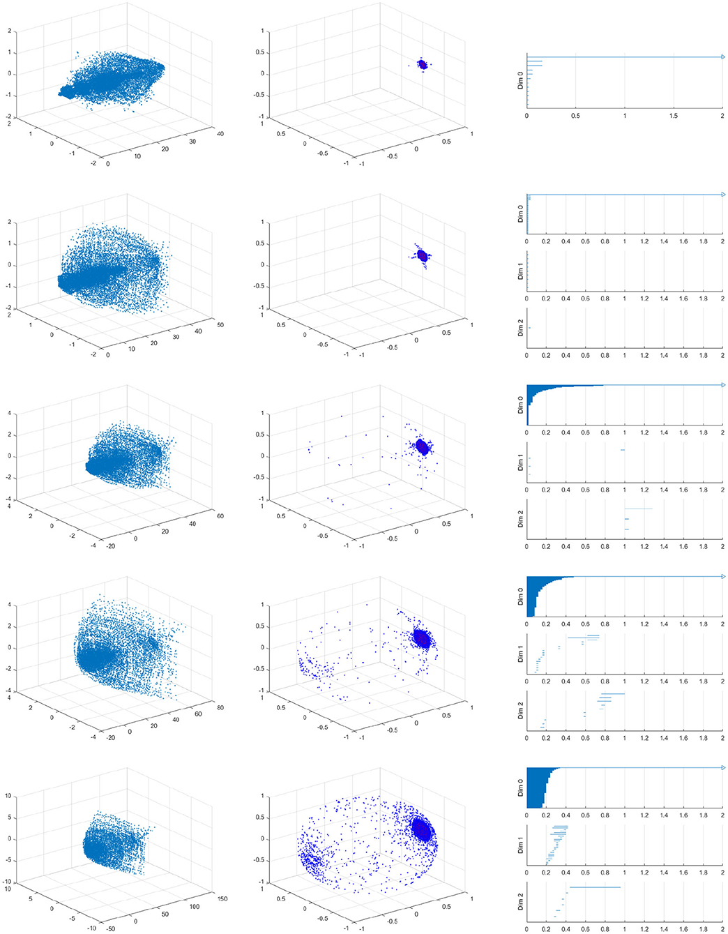
Figure A1. Velocity fields of symmetric vessel (left), the spherical projection (middle), and the corresponding barcode (right). 20, 30, 40, 50, 60% from top to bottom.

FIGURE A2

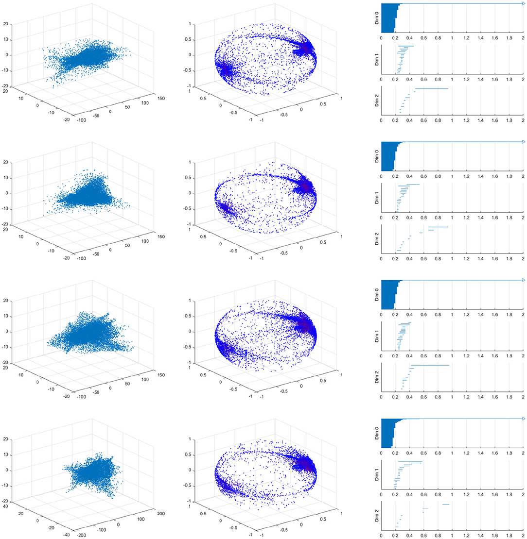
Figure A2. Velocity fields of asymmetric vessels (left), the spherical projection (middle), and the corresponding barcode with 40 by 20%, 40 by 30%, 40 by 50%, 40 by 60% stenosis from top to bottom.