Validation of Critical Ages in Regional Adult Brain Maturation

Introduction

It has previously been shown that many areas of the brain change non-linearly with age [1–3]. A critical age in development, therefore, can be defined as a point of transition between qualitatively different rates of change. The rates of change have often been compared to a linear and quadratic function of age with a significant contribution of the quadratic component indicating a non-linear change [4–6]. The magnitude of the rates of change have shown clear magnitude differences [2, 3, 7], but direct comparison between areas has been hampered by the fits used. Generally, regression procedures have been used to compare contributions of linear and quadratic components on fits to all the data (e.g., [1, 4]) which do not directly represent the rate of change for any particular age. However, more piecemeal, non-parametric spline fits have been used [2, 3, 6, 8, 9] that represent the specific rate of change for each age. Still, a validated procedure has yet to be demonstrated for both precisely determining the way a brain area changes with age and accurately determining when critical ages in development occur. Such a procedure can be shown theoretically for data with low noise levels but must also work for realistic noise levels. Since validation can only be determined in relation to a ground truth, here we test the procedures with simulated data before applying them to observed data.

The raw data from observed brain area volume is a combination of underlying developmental processes with individual variability in the timing and degree of those processes along with random measurement noise [10, 11]. Therefore, extracting the time course and structure of the development process for a particular brain area is non-trivial and likely requires multiple intermediate steps. Here the goal is to validate a set of steps that can result in a successful identification of the type of brain maturation that a particular brain area undergoes as well as the critical age that best indicates the key reflection point of the maturation. Validation of this model and falsification of other models will be based on the ability to extract ground truth measures. Invalid model performance can occur either by being mathematically inappropriate for a particular task or by a mismatch between the generated values and the ground truth values. For instance, one of the steps of the current procedure will be extracting derivatives of a smoothing spline. If it is shown that no particular derivative successfully extracts the critical age for a representative set of non-linear maturation patterns than any model that utilizes only a single derivative can be expected to misidentify the critical ages for certain patterns. However, it is not clear a priori how far off from the actual critical age such methods would be nor how often they may correctly apply to non-linear brain maturation patterns when they are only applied to experimentally observed data. Also, the smoothing spline is used here as a particular unbiased means of representing the curve to extract the critical ages [6]. Other bottom up approaches, such as PCA [12, 13], may be able to represent consistent components of the developmental time course, but may not be reliable in differentiating the maturation patterns, which would make them also insufficient to extract specific critical ages. Before discussing the new approach and validation of a method using smoothing splines, we will first discuss issues with using parabolic fits.

Adult brain maturation that proceeds at different rates across the lifespan has generally been indicated by acceleration of tissue loss in later life in particular brain areas (e.g., [14]). Though non-linear maturation can be demonstrated through the presence of a quadratic component in a parametric fit, parametric fits with quadratic components are unreliable as they are impacted by the range of ages used in the fit and therefore are likely to be inaccurate [6]. The inclusion of higher order parametric fits, such as cubic equations as done by Coupé et al. [15], would not necessarily resolve the reliability issues as they would also be impacted by the range of ages used in the fit. The benefit of their inclusion is that they can add new features, such as the presence and timing of plateaus in the maturation of gray matter. Non-parametric smoothing splines are more reliable across the range of ages used in a fit [6] and allow for the determination of critical ages where the rate of brain maturation changes [3]. Fjell et al. [3], put forth points of maximum change in maturation rate as the critical ages, which mathematically is equivalent to the zero points of the third derivative of the regional brain size. However, this process of determining critical ages has not yet been validated and can be shown to work well for only a subset of maturation patterns.

Here we will start with simulated data where the critical ages are specified mathematically so that the precise critical ages are known, then the reliability and accuracy of using different components of the fits will be compared. Theoretically different patterns of brain maturation can occur that have been empirically demonstrated. Linear volume change is typically shown as a constant decrease in size, such as in the nucleus accumbens [5]. The maturation rate, i.e., first derivative of regional brain size, is a constant non-zero value across age and therefore the higher derivatives are all a constant zero value (see Figure 1, “Curve Type 0”). Non-linear volume changes have derivatives with at least some non-zero values across age.

FIGURE 1

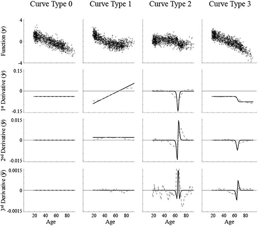
Figure 1. Simulated data along with the first three derivatives of the best fit smoothing spline (gray dashed lines). The actual curve (black solid line) that the simulated data is based on is shown in the first derivative row. A medium level of noise (σ = 0.5) was used. The critical age for all non-linear curves is 65. Curve Type 0 has a constant first derivative, aka maturation rate, with no critical age. Curve Type 1 has a linear maturation rate with a critical age at the 1st derivative zero point. Curve Type 2 has a Gaussian maturation rate with a critical age at a 2nd derivative zero point. Curve Type 3 has a sigmoidal maturation rate with a critical age at a 3rd derivative zero point.

One non-linear trajectory is a U-shaped pattern with a switch from decreasing size early in adulthood to increasing size later in adulthood, as in the caudate nucleus [3], or similarly an inverse U-shaped pattern with a period of increasing size followed by decreasing size, such as in global white matter [1, 15, 16]. The maturation rate increases or decreases linearly as a function of age. The point of inflection where the direction of change in size reverses would be reflected as a zero point of the first derivative. Higher derivatives fluctuate with age and typically have more than one zero point (see Figure 1, “Curve Type 1”). A second type of pattern involves a sigmoidal shape, where there is a restricted age period with a lot of change though there is little to no change before and after this period, or a basic cubic function, which has a plateau in the middle with very little change or constant change before and after the plateau, such as in the pallidum [3] or global gray matter [15]. The maturation rate would be in the shape of a Gaussian curve with a clear peak or trough. The location of the maximum or minimum maturation rate would be reflected as a change in direction of the maturation rate, which is a zero point of the second derivative. As smoothing splines tend to be locally curvy, zero points would exist for first and third derivatives also, though they may occur at different ages (see Figure 1, “Curve Type 2”). A third type of pattern is where there is a transition from one rate of change to another though the direction of change remains the same, such as an acceleration in the rate of brain maturation shown in the lateral ventricles [3]. The maturation rate would be sigmoidal with a sharp discontinuity at the point of change, which is a change in concavity of the rate of change, i.e., a zero point of the third derivative. Though there would not likely be first derivative zero points due to the maturation rate always being of the same sign, second derivative zero points could occur for age regions with a constant maturation rate due to imperfect, curvy fits (see Figure 1, “Curve Type 3”).

Given that different components of the rate of brain maturation would most directly apply to the different patterns of brain maturation, i.e., the zero points of the first, second, or third derivative of the regional size, here we will explore various questions in regards to how well the critical age can be determined based on a single derivative for each pattern. For instance, can the third derivative of the regional brain size, as proposed by Fjell et al. [6], and used by Fjell et al. [3] and Zeigler et al. [8], accurately and reliably determine the critical age for each pattern of brain maturation? If not, can the type of pattern be consistently determined such that the appropriate component can be applied? If the appropriate component is applied, how accurately can the actual critical age be determined? And finally, does a re-evaluation of the Fjell et al. [3], data using the component that best matches the type of brain maturation pattern indicate the same or different critical ages for the various regions analyzed?

Methods

Types of Data

Biological Data

For this study, de-identified and z-scored cross-sectional data was provided by Anders Fjell under a data processing agreement. The collection and processing of the data is discussed in Fjell et al. [3]. Briefly, it consisted of 1,100 data points for each of 17 brain measures from adults ranging in age from 18 to 94 years old (mean age = 47.7, standard deviation = 19.7). More specifically, the data is for the 12 non-linear measures of the brain shown in Figure 9 and five linear brain areas (plots of these measures can also be found in Figures 1, 2 of [3]). The smoothing spline fits used to determine their reported critical ages were not provided. The variability in the data was determined by first fitting a smoothing spline and then calculating the standard deviation of the residuals from the actual z-scored magnitude in relation to the spline fit.

Generated Data

Simulated data with known brain maturation patterns was generated in order to test the validity of using particular derivatives of the smoothing spline for estimating critical ages in various patterns. Four particular patterns were examined, one linear function with no critical age and three non-linear functions that each had a single critical age corresponding to different derivatives of the smoothing spline.

1) A linear function of age (see Figure 1, “Curve Type 0”) has a constant derivative, or slope, and is represented by the function

$\begin{array}{ll}\text{y}=a\text{x},& (1)\end{array}$

with x as the age, y as the z-scored brain area size, and a constant brain maturation rate, i.e., first derivative or slope, of

$\begin{array}{ll}\dot{\text{y}}=a.& (2)\end{array}$

2) A quadratic non-linear function of age (see Figures 1–3, “Curve Type 1”),

$\begin{array}{ll}\text{y}=b{(\text{x}-x_{crit})}^2,& (3)\end{array}$

FIGURE 2

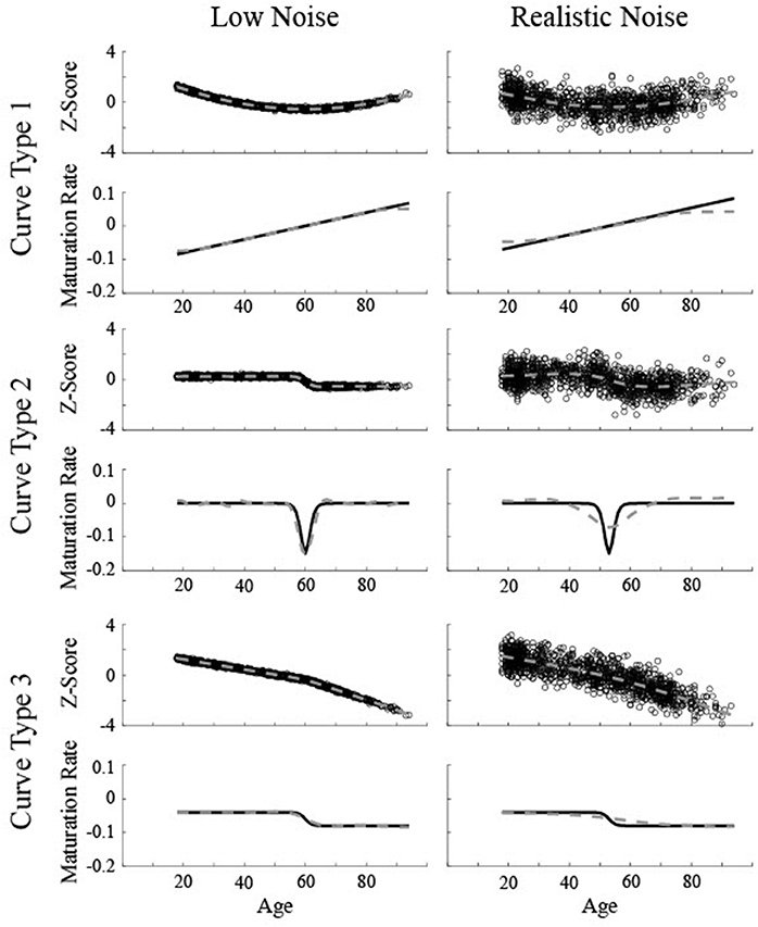
Figure 2. Simulated data created based on three different curves for two different levels of noise (Low Noise, σ = 0.075, and Realistic Noise, σ = 0.75). Top rows represent volume (z-score) and the bottom rows show the actual instantaneous slope (maturation rate: $\dot{\text{y}}$). Dotted gray lines show the smoothing spline fit. The critical age for all three low noise curves is 60. The critical age for all three realistic noise curves is 53.

FIGURE 3

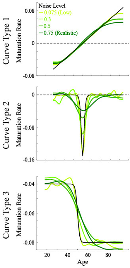
Figure 3. Simulated maturation patterns for multiple noise levels based on three non-linear curve types. Solid black lines show the actual maturation pattern. Green lines show the 1st derivative of the smoothing spline fit to data of various noise levels. The critical age for all curves is 50.

represents an accelerating non-linearity which has a linearly changing slope such that the brain maturation rate varies with age,

$\begin{array}{ll}\dot{\text{y}}=2b(\text{x}-x_{crit}),& (4)\end{array}$

and a clear critical age at x_crit. For such a U-shaped function, this would be equivalent to the maturation rate switching from positive to negative or negative to positive and the critical age is the zero point of the first derivative.

3) A sigmoidal non-linear function of age (see Figures 1–3, “Curve Type 2”),

$\begin{array}{ll}\text{y}=\frac{c}{1-e^{-(\text{x}-x_{crit})}},& (5)\end{array}$

represents developmental patterns with a temporally restricted period of change. The slope is a Gaussian function,

$\begin{array}{ll}\dot{\text{y}}=\text{y}(1-\text{y}),& (6)\end{array}$

with the center of the sigmoid, x_crit, having a local maximum or minimum in slope, $\ddot{\text{y}}=0$, and neighboring points having a change in concavity, $\stackrel{⃛}{\text{y}}=0$. Therefore, the zero point of the second derivative uniquely defines the critical age as the center of the temporal period of change.

4) A temporally isolated non-linearity (see Figures 1–3, “Curve Type 3”) has a change in the magnitude of an otherwise constant maturation rate,

$\begin{array}{ll}\text{y}=d_1(\text{x}-x_{crit})+f_1\text{for}\text{x}\le x_{crit},& (7)\end{array}$

$\begin{array}{ll}\text{y}=d_2(\text{x}-x_{crit})+f_2\text{for}\text{x}>x_{crit},& (8)\end{array}$

whose continuous slope can be approximated by a sigmoidal function,

$\begin{array}{ll}\dot{\text{y}}=d_1+\frac{d_2-d_1}{1-e^{-(\text{x}-x_{crit})}}.& (9)\end{array}$

The center of the sigmoid, x_crit, is the critical age of the non-linearity and corresponds to a change in concavity of the maturation rate, which is the zero point of the third derivative.

Each curve was simulated 250 times for each of two values of random noise. The specific ages of each data point corresponded to the observed ages in the biological data and the “realistic noise” level of 0.75 was determined based on the average standard deviation of the observed data points from the best fit smoothing spline (see “Determination of Noise Levels” for more details). A separate set of “realistic noise” data was created using uniformly distributed ages in order to test the performance of the method without the impact of a lower distribution of data at the oldest ages. A second “low noise” level was included with 1/10 the standard deviation to assess how well the procedures worked under very high signal to noise ratios. The critical age for each simulation was randomly chosen from a uniform distribution with a minimum age of 45 and a maximum age of 75. The magnitudes of the maturation rate for the different maturation patterns were held constant across simulations to approximate the effect sizes observed in the biological data. The specific values were: a = −0.04, b = 0.001, c = −0.8, d₁ = −0.04, d₂ = −0.08. Note that in the process of classifying the curve type, the maturation rate was normalized and slopes for half of the simulations were inverted such that the particular effect size and direction of the maturation pattern were irrelevant.

Analysis Steps for Top-Down, Theory Driving Curve Fitting

Smoothing Spline Fitting

Using MATLAB R2018a with the Curve Fitting Toolbox installed, the best fitting non-parametric smoothing spline [6, 8] was determined for each simulation of each maturation pattern. The smoothing parameter, which constrains the number of knots used to fit the data, was determined based on the minimum Bayesian Information Criterion (BIC), using the equation

$\begin{array}{ll}BIC=nlog(SSE)+(n-1)log(n)& (10)\end{array}$

with n = number of knots in the spline. Smoothing parameters were checked for 1000 logarithmically spaced points between 10⁻⁷ and 10⁻¹ such that the sum of squared error (SSE) tended to decrease as the value of n increased, but using the minimum BIC ensured that the value of n did not get too high as it was constrained by the amount of noise in the data, which is reflected in the SSE. A continuous estimate of the z-scored brain size along with its first derivative (i.e., maturation rate), second derivative, and third derivative based on the smoothing spline was then determined for the 119 unique, monotonically increasing ages from the biological data. To ensure that the results were not contingent on noisy calculations of the derivatives, analyses were repeated for smoothed versions of the 2nd and 3rd derivatives. Smoothing was done with a sliding window that averaged together the current age point and the two adjacent age points on each side. Examples of the smoothing spline fits for different noise levels are shown in Figures 1–3 and examples of the smoothed 3rd derivative are shown in Figure 10.

Determination of Critical Ages

The smoothing spline fits were used to estimate critical ages based on the zero points of the first, second, and third derivatives. First, the age for any zero point was determined as a change in sign of the derivative from that age to the next age. High levels of specificity, which would be indicated by a single critical age guess per curve, were tested by examining the proportion of simulations resulting in no zero points, one zero point, or more than one zero point. A consequence of the smoothing spline procedure is that a continuous function is generated with smooth transitions between points such that curved lines result even if the ground truth-generated maturation pattern is a straight line (see Figure 1). Therefore, multiple zero points are likely to occur for the various derivatives of the smoothing spline even if the ground truth pattern has only a single zero point for a given derivative. To output a single critical age guess based on each derivative, other derivatives were used to systematically constrain the output. Multiple first derivative zero points were expected to occur only when the maturation rate was constant and near zero, i.e., there is no real critical age of interest. Therefore, an arbitrary procedure was used such that the critical age based on the first derivative zero point was chosen to minimize the absolute value of the second derivative at that point, i.e., be a local maximum or minimum of the slope. Multiple second and third derivative zero points were expected to occur due to the nature of the fitting procedure itself, which results in curves with more peaks for lower noise levels (Figure 3). Therefore, procedures were used to identify the most prominent zero point in relation to the preceding derivative. The critical age based on the second derivative zero point was chosen to be the most distinct slope, i.e., the furthest from the average first derivative. The critical age based on the third derivative zero point was chosen to maximize the second derivative, i.e., the point of greatest change in slope.

Classification of Curve Type

Different curve types are based on different underlying maturation patterns and were expected to require different derivative zero points to be applied in order to identify the relevant critical ages. Therefore, a means was sought to determine which maturation pattern best matched a particular simulation. The slope of the smoothing spline, i.e., the maturation rate, for 77 equally spaced, whole number ages from 18 to 94 was used as input to the classification system. This measure was chosen to disentangle the input from the specific set of observations used in order for the process to be more broadly applicable across future research studies. Additionally, a 78th input value not related to age was included in order to assist in differentiating linear and non-linear maturation patterns. That is, a categorical variable, i.e., a value of 0 or 1, was included of whether or not the standard deviation of the curve was <0.005, as linear maturation patterns have a constant maturation rate (standard deviation of 0). The Classification Learner within MATLAB R2018A was used on simulated data to determine which type of classifier worked best using a 5-fold cross-validation procedure for data with 250 trials for each of the 4 curve types. A quadratic Support Vector Machine [17, 18] most consistently worked best across multiple samples of simulated data. A set of “medium noise” data (standard deviation of 0.5) was used to build a classifier that could then be applied to other data sets, specifically the low noise simulated data, realistic noise simulated data, and biological data. See “Comparison of Different Classifiers” for more details on the different options explored and how these specific values were chosen.

Assessing Consistency Between Calculated and Actual Critical Ages

A known but variable critical age value was used in the generation of data for the validation process of the procedures described above. This allows for a quantitative comparison between the calculated critical age guess and the actual critical age used to generate the data. Two methods of assessment were used—the proportion of guesses within 5 years of the critical age, which is a binary measure to emphasize the clinical applicability of the process, and the root mean squared error (RMSE), which is a continuous measure to characterize the magnitude of discrepancy across all data points. Specifically, the RMSE was calculated using the equation

$\begin{array}{ll}RMSE=\sqrt{}{\displaystyle \sum _{i=1}^n}\frac{{(y_i-x_i)}^2}{n},& (11)\end{array}$

with n = number of simulations, y = critical age guess, and x = actual critical age.

Analysis Steps for Bottom-Up, Model Free Curve Fitting

PCA on Smoothing Splines

In order to determine if there is sufficient information contained within the time courses of the maturation patterns to differentiate them (e.g., [12]), principal component analysis (PCA) was done on the generated data using MATLAB 2018a. The input was 77 time points of the smoothing spline for each of 1,000 time courses (250 per curve type). PCA analysis was run separately for the different noise levels. The primary outputs were all principal components, ordered by the amount of variance explained (see Figure 11), and the relative scaling scores of the different principal components, which were used for statistical comparison between the curve types. A one-way ANOVA was run for each of the first five principal components, with curve type as the factor, using SPSS 26. A cutoff of p < 0.001 was used to determine statistically significant levels of information for differentiating curve types due to multiple comparisons [19].

PCA on FFT of Smoothing Splines

Given the distribution of critical ages within the generated data set, it was expected that the phase of the curves needed to be accounted for in addition to their shape over time. Fast Fourier transform (FFT) was first applied to the smoothing spline to conduct spectral PCA on the power spectra or the combination of the power and phase spectra (e.g., [20]). PCA was run using the same steps as described in “PCA on Smoothing Splines,” but with different input. Of note is that the FFT procedure was run with additional padding of zeros after the smoothing spline in order to have the length of the time course be a power of 2, in this case 128 time points. The resulting power spectra is symmetric such that only the average of the time course and half of the available frequencies provide distinct values, in this case a total of 65.

Input type 1 was the amplitude of the power spectra, which contained 65 data points. Input type 2 was the power spectra combined with the raw phase spectra, for a total of 130 data points. The power spectra and phase spectra were separately normalized to each have a mean of 0 and standard deviation of 1 prior to combining in order to allow for equal contribution toward the principal components. Input type 3 was the normalized amplitude of the power spectra combined with the normalized unwrapped phase spectra, for a total of 130 data points. The unwrapping process removes sharp discontinuities in phase values for nearby frequencies that can result due to the conversion of radial phase to a linear number line. This can better allow for consistencies in phase relationships across frequencies to be picked up by the PCA.

Results

Determination of Noise Levels

The amount of noise typically present in experimentally observed data was sought in order to generate simulated data using biologically realistic noise levels. First, a smoothing spline was determined for each of the 17 areas of the Fjell et al. [3], data (see “Biological Data”) and the residuals of each data point in relation to the smoothing spline was calculated. Then the standard deviation of the residuals was calculated for the entire time course to indicate the amount of noise. Noise levels ranged from 0.61 (cerebral cortex) to 0.98 (fourth ventricle), with an average of 0.80 and standard deviation across areas of 0.11. However, variability tended to be higher in the older ages than younger ages, particularly in the ventricles (see Figure 9). Therefore, the standard deviation of the residuals was recalculated for ages <70. Within this age range, noise levels ranged from 0.49 (inferior lateral ventricle) to 0.95 (fourth ventricle), with an average of 0.75 and standard deviation across areas of 0.13. This value of 0.75 was used as the “realistic noise” level for generated data.

Results of Top-Down Method for Generated Data

To determine whether particular derivatives of a smoothing spline were informative regarding the actual critical ages in generated maturation patterns, multiple analyses were done. The specificity of the derivatives was estimated through the number of zero points of each derivative for each type of curve. The accuracy and reliability of a determined best guess, i.e., a single critical age guess per derivative regardless of the number of zero points, was assessed through comparison to the actual critical age. The validity was confirmed through the ability to classify the type of curve in order to extract the critical age guess based on the relevant derivative.

Number of Zero Points

Overall, the number of critical age guesses, i.e., number of zero points of the derivative, varied substantially between the types of curves and the specific derivative (Figure 4). To assess variation in specificity across curve type and derivative, a 3 × 3 × 2 mixed-model ANOVA was run with derivative type as a within-subjects factor (1st, 2nd, and 3rd) and curve type (1, 2, and 3) and noise level (realistic and low) as between-subject factors. All main effects and interaction effects were significant (all F's > 90, all p's < 0.001). 3rd derivatives had the highest number of zero points (average of 18.4) whereas 1st derivatives had the lowest number (3.0) and 2nd derivatives had a middle level (6.6). Curve Type 2 had the highest number of zero points (16.0) whereas Curve Type 1 had the lowest number (4.8) and Curve Type 3 had a middle level (7.2). Low noise curves had more zero points than high noise curves [13.6 vs. 5.0, F_{(1, 1494)} = 86001.0, p < 0.001]. That is because lower levels of noise allow for a greater number of knots in the BIC minimization procedure, resulting in more local peaks, though higher noise generally leads to smoother splines with less zero points but also less consistency with the actual maturation rate. As seen in Figure 3, the smoothing spline fits for higher levels of noise tended to flatten out as a function of age in relation to lower noise data. Smoothing the 2nd and 3rd derivative curves prior to determining the zero points reduces the overall number of zero points, but the general patterns remain of an increase in zero points for lower noise and a higher number of zero points for the 3rd derivative than the 1st and 2nd derivatives (Figure 4).

FIGURE 4

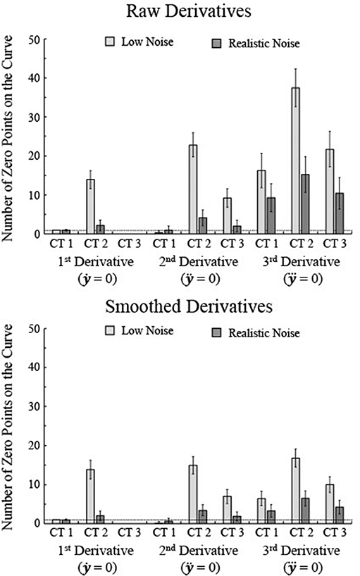
Figure 4. The number of zero points for each of the first three derivatives was determined for 250 simulations each of three types of curves, separately for raw 2nd and 3rd derivatives and smoothed 2nd and 3rd derivatives. Smoothing was done using a sliding window that averaged the five nearest age points. Note that the number of zero points tends to increase as the noise level decreases even though the fits better match the actual maturation rate for lower levels of noise. The horizontal line indicates one zero point. Error bars show one standard deviation.

High specificity would be shown by a single critical age guess per curve. The 1st derivative of Curve Type 1 with low noise was the only combination that always resulted in a single zero point for all trials (Figure 4), though the 1st derivative of Curve Type 1 with realistic noise had an average of 0.96 zero points and the 2nd derivative of Curve Type 1 with realistic noise had an average of 0.996 zero points. The 1st derivative of Curve Type 3 for both low and realistic noise never had zero points and the 2nd derivative of Curve Type 1 averaged 0.28 zero points across trials (see Figures 4–6). All other combinations of derivative, curve type, and noise level resulted in significantly more than one zero point per curve (all one-sample t's > 10.9, p's < 0.001). When the 2nd and 3rd derivative curves were smoothed, the 1st derivative of Curve Type 1 was the only combination that consistently resulted in a single zero point.

FIGURE 5

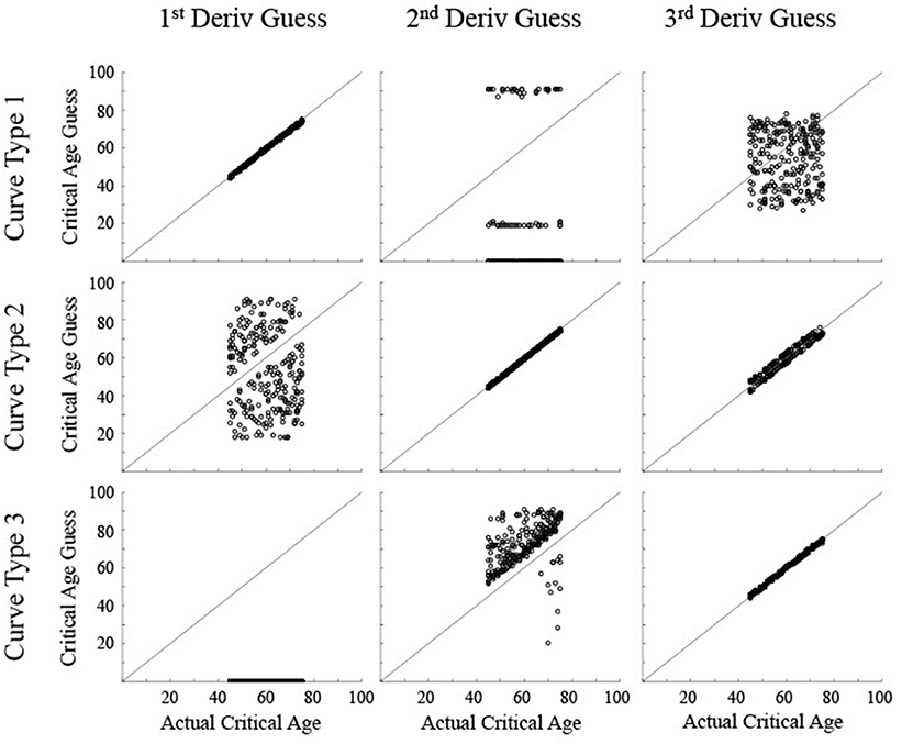
Figure 5. Scatter plots show the critical age guesses for the Low Noise data (σ = 0.075) for each of the first three derivatives for each type of curve. Points along the diagonal line indicate a match between the calculated critical age and the actual critical age of the stimulated data. Points along the x-axis indicate no derivative zero points for that trial.

FIGURE 6

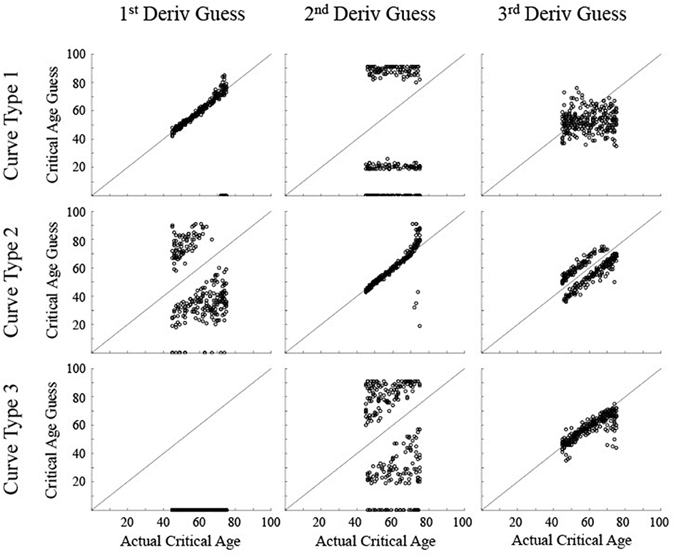
Figure 6. Scatter plots show the critical age guesses for the Realistic Noise data (σ = 0.75) for each of the first three derivatives for each type of curve. Points along the diagonal line indicate a match between the calculated critical age and the actual critical age of the stimulated data. Points along the x-axis indicate no derivative zero points for that trial.

Analysis Using Zero Points of a Single Derivative

Various patterns of how the calculated critical age guess corresponded to the actual critical age defined by the specified maturation rate were observed for different pairings of the type of curve and the particular derivative used as the basis of the critical age guess (see Figures 5, 6). As will be detailed below, generally the calculated critical age was consistent with the actual critical age when the derivative used matched the relevant type of curve and was inconsistent otherwise. Smoothing the 2nd and 3rd derivative curves did not qualitatively change the results as the most prominent zero point was used as the calculated critical age regardless of how many zero points occurred (see “Determination of Critical Ages”).

For the low noise simulated data (Figure 5), the calculated critical age was always within 5 years of the actual critical age when the particular derivative matched the type of curve, with a root mean squared error (RMSE) of 0.55 or less, evidenced by the guesses clustering along the diagonal line for each of the subfigures along the upper-left to bottom-right diagonal. The 3rd derivative guesses also closely corresponded to the critical age for Curve Type 2, with 100% of the guesses within 5 years, though the RMSE of 2.2 also indicates that they were generally slightly off of the diagonal line. The 3rd derivative guess was disconnected from the actual critical age for Curve Type 1 as the guesses were uniformly distributed between 30 and 80 regardless of the actual critical age, resulting in a RMSE of 17.4. The 2nd derivative guess was also disconnected from the actual critical age for Curve Type 1, but in this case the zero points, when present, were at the most extreme values of the age range, resulting in a RMSE of 32.5. The 2nd derivative guesses for Curve Type 3 tended to cluster above the actual critical age (average residual was 11.7, RMSE of 11.0), indicating they tended to occur after the change in maturation rate (see Figure 3). The 1st derivative guess, though valid for Curve Type 1, was disconnected from the actual critical age for Curve Type 2 (RMSE of 23.8) and did not have any guesses for Curve Type 3.

For the realistic noise simulated data (Figure 6), the calculated critical age was consistently within 5 years of the actual critical age when the particular derivative matched the type of curve (92% for 1st derivative guesses for Curve Type 1, 90% for 2nd derivative guesses for Curve Type 2, and 77% for 3rd derivative guesses for Curve Type 3), consistent with the guesses clustering along the diagonal line for each of the subfigures along the upper-left to bottom-right diagonal. However, there was more spread in the guesses for realistic noise data compared to low noise data (RMSE of 2.1 for 1st derivative guesses for Curve Type 1, 6.4 for 2nd derivative guesses for Curve Type 2, and 5.2 for 3rd derivative guesses for Curve Type 3 vs. <0.55 for all curve types with low noise). This is because correlations between the smoothing spline fit and the actual maturation rate curve were consistently lower for the realistic noise simulated data in relation to the low noise simulated data (average correlations—low vs. high: Curve Type 1: 0.998 vs. 0.989; Curve Type 2: 0.959 vs. 0.574; Curve Type 3: 0.994 vs. 0.936). The 3rd derivative guesses were now further from the critical age for Curve Type 2, with only 8% of the guesses within 5 years and a RMSE of 7.4. The 3rd derivative guess was again disconnected from the actual critical age for Curve Type 1 as the guesses were still uniformly distributed, but were now more clustered around the mean age, resulting in a RMSE of 11.8. The 2nd derivative guess was also disconnected from the actual critical age for Curve Type 1 but the zero points, when present, were largely clustered at the most extreme values of the age range, resulting in a RMSE of 39.9. The 2nd derivative guesses for Curve Type 3 tended to cluster more symmetrically around the actual critical age but were always away from the actual critical age (RMSE of 35.6), indicating they occurred equally often before and after the change in maturation rate (see Figure 3). The 1st derivative guess, though still valid for Curve Type 1, was still not valid for Curve Type 2 (RMSE of 26.4) and did not have any guesses for Curve Type 3.

Comparison of Different Classifiers

As initial results indicated that the critical age guess consistently matched the actual critical age for only one of the derivative zero points for each curve type (Figures 5, 6), a means was sought to determine the curve type from the observed smoothing spline. This categorization process includes the linear maturation rate of Curve Type 0 shown in Figure 1 and allows for identification of the appropriate derivative zero point using only the observed data. Using generated data with various levels of noise from 0.07 to 0.75, the performance of all available classifiers in the Classification Learner within MATLAB 2018a was assessed (Table 1). The specific input to the classifier was the normalized slope of the smoothing spline for 77 ages plus the variability of the slope across all ages for each set of generated data (see “Classification of Curve Type”). Performance generally improved as the noise level decreased, resulting in above 95% accuracy for multiple models, though accuracy remained low for linear classifiers (accuracy was always below 50%, with chance level at 25%). Averaged across all noise levels tested, the Quadratic SVM resulted in the highest level of performance (85%), though the weighted KNN and Ensemble-Bagged Trees classifiers performed similarly (84%).

TABLE 1

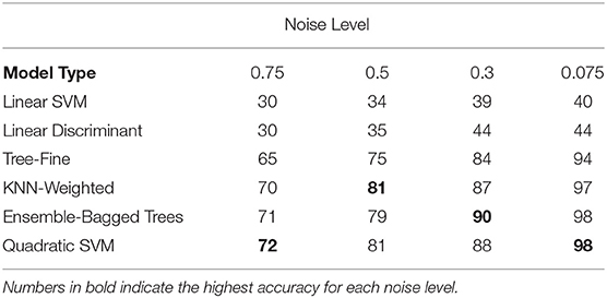
Table 1. Classification accuracy for a subset of tested classifiers for a range of noise levels (chance is 25%).

The performance of the different classifiers was initially assessed on each set of data separately. A single classifier was sought that could be applied effectively across both realistic and low levels of noise though classifiers tend to generalize best to similar noise levels due to idiosyncrasies in the smoothing splines for different noise levels (see Figure 3). Therefore, the classifier trained for each level of noise using the Quadratic SVM was applied to both low and realistic noise data (Figure 7). In conjunction, a threshold was sought for the variability along the spline to aide in the differentiation between linear and non-linear curves since the variance for Curve Type 0 ought to be near 0. In general, classification initially improved for realistic noise data when a relatively low standard deviation threshold was used (74% correct at 0.0001), remained consistent and high for a wide range of thresholds (accuracy was 89% or above from 0.0003 through 0.007), and then decreased as the threshold increased (78% at 0.02). Two particular values from the plateau region were compared that were selected based on different criteria. The threshold of 0.0003 had the highest discrimination between the linear Curve Type 0 being below threshold and the non-linear curves being above threshold. Specifically, 96% of the linear Curve Type 0 while <3% of Curve Type 3 and 0% of Curve Types 1 and 2 were below the threshold. Looking at the biological data, the five linear areas had observed standard deviation values of 0.0041 or below whereas the 12 non-linear areas had observed standard deviation values of 0.0095 or above. Therefore, a threshold of 0.005 was utilized, for which 100% of the simulated trials of the linear Curve Type 0 but 3% of Curve Type 3 and 0% of Curve Types 1 and 2 were below the threshold.

FIGURE 7

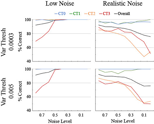
Figure 7. Classification accuracy as a function of noise level, shown separately for low and realistic noise levels and two levels of variance threshold. Percent correct of 250 trials per data point is shown for the four different curve types along with the overall percent correct across curve types. Chance is at 25%.

As anticipated, performance for the low noise data remained high for a range of classifiers based on different noise levels though it started to come off of the ceiling around a noise level of 0.4 and dropped below 80% accuracy for one or more curve types by 0.7 for both variance threshold levels (Figure 7). The performance for the realistic noise data started off lower initially and decreased performance fast as the noise level decreased (Figure 7). Performance started to systematically drop below 80% for one or more curve types starting at 0.4 for a threshold of 0.005 and at 0.5 for a threshold of 0.0003. Furthermore, accuracy for the linear Curve Type 0 was consistently higher and essentially 100% for a threshold of 0.005. Therefore, to maximize correct classification of linear vs. non-linear curves and to balance the performance at low and realistic noise levels, a classifier trained with 0.5 noise and a threshold of 0.005 was utilized below for analyzing both the generated data and the biological data.

Determination of Curve Type and Critical Age

For the final validation step on using a smoothing spline to determine the critical age in a maturation pattern, the performance of a classification procedure was assessed to automatically determine the type of curve so that the appropriate derivative could be ascertained (see “Classification of Curve Type”). For the low noise data (Figure 8), the correct type of curve was identified 99.7% of the time (3 of the Curve Type 3 trials were incorrectly classified as Curve Type 2), consistent with the high levels of correlation between the smoothing spline and the actual maturation pattern (the correlation coefficient for all trials was >0.95). For the realistic noise data (Figure 8), classification performance varied by curve type but was consistently well above chance. The lowest performance was for Curve Type 2 at 80% correct, which was misclassified on the remaining trials as Curve Type 3. Curve Type 1 had 93% accuracy, though on 7% of trials it was misclassified as Curve Type 3. Curve Type 3 was classified correctly on the vast majority of trials (82% correct), though incorrect trials were split between Curve Type 1 (7%) and the linear maturation rate (11%). The linear maturation rate, i.e., Curve Type 0, was correctly classified on 100% of trials. For the realistic noise data with a uniform distribution of ages, classification accuracy improved—Curve Type 1 was 98% correct, Curve Type 2 was 92% correct, Curve Type 3 was 94% correct, and Curve Type 4 was 100% correct. These results indicate that the classification procedure can consistently differentiate between types of maturation patterns.

FIGURE 8

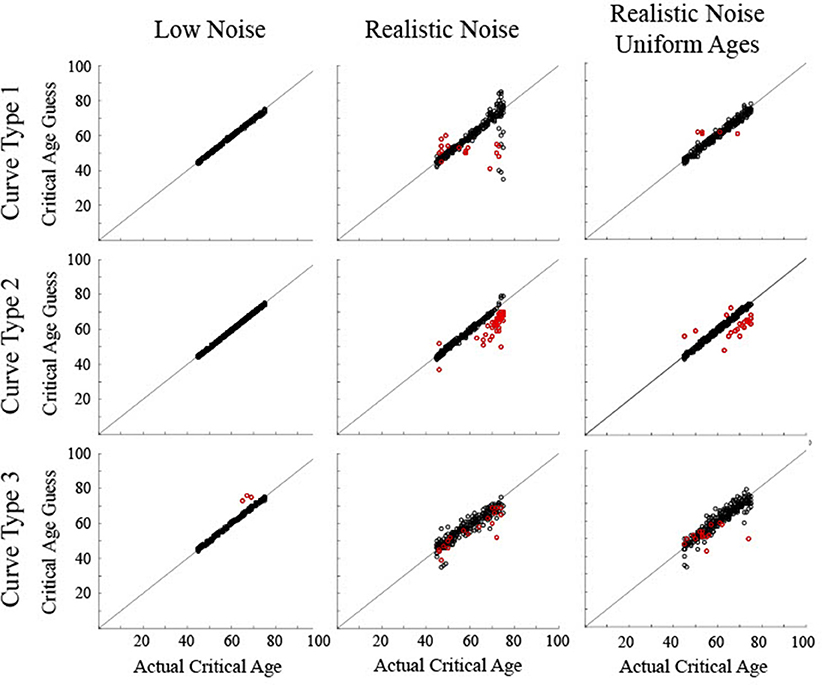
Figure 8. Scatter plots show the critical age guesses for the simulated data following a classification procedure to determine which particular derivative zero point to use. Black circles show correct classification of curve type. Red circles show incorrect classification of curve type. Points along the diagonal line indicate a match between the calculated critical age and the actual critical age of the stimulated data.

The validity of the output of the classification procedure was determined by comparing the calculated critical age against the actual critical age (Figure 8). Note that in order to provide a critical age guess for the Curve Type 3 trials that were misclassified as a Curve Type 1, since there was no first derivative age guess for these trials, the third derivative age guess was used whenever a trial was classified as a Curve Type 1 but there was no first derivative guess. This had the unintended consequence of also causing some Curve Type 1 trials that were correctly classified as Curve Type 1 to use the third derivative guess when there was no first derivative zero point. This occurred when the maturation rate approached but did not quite reach a value of 0 such that the sign of the first derivative never changed. This occurred for 3% of the Curve Type 1 trials with realistic noise.

For the low noise simulated data, all determined critical ages for Curve Type 1 and Curve Type 2 and 99% of determined critical ages for Curve Type 3 were within 5 years of the actual critical age (all RMSE <1.0). The 3 incorrect trials for Curve Type 3 were biased above the curve (average residual of 7.7, RMSE of 1.5). For the realistic noise simulated data, the consistency between the determined critical age and the actual critical age varied as a function of curve type. For Curve Type 1, 89% of the determined critical ages were within 5 years of the actual critical age, including 93% of the correct trials but only 29% of the incorrect trials. The correct trials were not biased (average residual of −0.6, RMSE of 5.1), but the incorrect trials were biased toward the middle of the age range (average residual of −6.1, RMSE of 12.5). For Curve Type 2, 90% of the determined critical ages were within 5 years of the actual critical age, including 100% of the correct trials but only 8% of the incorrect trials. The correct trials were not biased (average residual of −0.4, RMSE of 1.0), but the incorrect trials were biased below the actual critical age (average residual of −8.1, RMSE of 4.1). For Curve Type 3, 74% of the determined critical ages were within 5 years of the actual critical age, including 86% of the correct trials but only 20% of the incorrect trials. The correct trials were not biased (average residual of −0.8, RMSE of 3.2), but the incorrect trials were biased below the actual critical age (average residual of −4.7, RMSE of 4.9). For the realistic noise simulated data with uniform ages, a higher percentage of critical ages were within 5 years of the actual critical age−98% for Curve Type 1, 92% for Curve Type 2, and 90% for Curve Type 3. Additionally, determined critical ages were closer to the actual critical age for Curve Type 1 (RMSE of 1.8) and Curve Type 2 (RMSE of 2.7), though were similar for Curve Type 3 (RMSE of 3.5).

Results for Biological Data

Critical ages for cross-sectional MRI data from 17 brain measures (see “Biological Data”) were found using the same classification procedure as was applied to the simulated data. That is, the type of curve was first determined based on the smoothing spline fit and then the relevant derivative zero point was chosen as the critical age. The determined critical ages were then compared to those reported in Fjell et al. [3], which always used 3rd derivative zero points of a smoothing spline fit as the critical ages. However, the exact method of defining the smoothing spline, i.e., the constraint on the smoothness defined by the BIC vs. AIC, may have resulted in enough differences in the local bumps of the smoothing spline to account for some differences in the determined critical ages. Therefore, discussion of the results will extend to aspects of the maturation pattern that are consistent or inconsistent between the methods.

Classification of Curve Type

At least one brain area was classified as belonging to each of the maturation patterns with the majority (10/17) belonging to Curve Type 3, one classified as Curve Type 1 (caudate nucleus), one classified as Curve Type 2 (pallidum), and five classified as Curve Type 0, i.e., linear (cerebellum cortex, thalamus, putamen, amygdala, and nucleus accumbens).

Comparison of Specified Critical Ages

The five areas classified as linear were consistent between the current method and Fjell et al. [3]. To help compare between the results for the non-linear areas, the critical ages based on both are shown for 12 areas in relation to the raw data and maturation pattern (Figure 9) and the 3^rd derivative curve (Figure 10). For the caudate nucleus, identified as a Curve Type 1, the critical age guesses are within 1 year (59 vs. 60). The 3rd derivative zero point was in a similar range (55) as that is the point of maximum curvature change for the maturation rate. For the pallidum, identified as a Curve Type 2, the critical age guesses occur along different points of the curve—the 2nd derivative zero point is the peak of the maturation rate curve (59) whereas the 3rd derivative zero points are near symmetrically offset around the peak (49 and 70), corresponding to the middle of the rise and fall of the maturation rate. For two of the curves identified as Curve Type 3 (total brain volume and cerebral cortex), the critical age guesses are within 3 years of one another across methods as both points are in the vicinity of the point of maximum curvature change for the maturation rate. For the other eight curves identified as Curve Type 3, the Fjell et al. critical age guesses did not clearly correspond to the calculated 3rd derivative zero points, but sometimes corresponded to peaks of the 3rd derivative (e.g., lateral ventricles, fourth ventricle, brain stem, hippocampus), a 3rd derivative zero point that was distinct from the most prominent 2nd derivative peak (e.g., cerebellum white matter), or an age that was not clearly identifiable based on the smoothing splines calculated here (e.g., lateral inferior ventricle, third ventricle, cerebral white matter). To better clarify the correspondence of any particular critical age guess with the calculated 3rd derivative zero points, Figure 10 shows a smoothed version of the 3rd derivative along with the determined critical ages based on the methods described here and those reported in Fjell et al. [3].

FIGURE 9

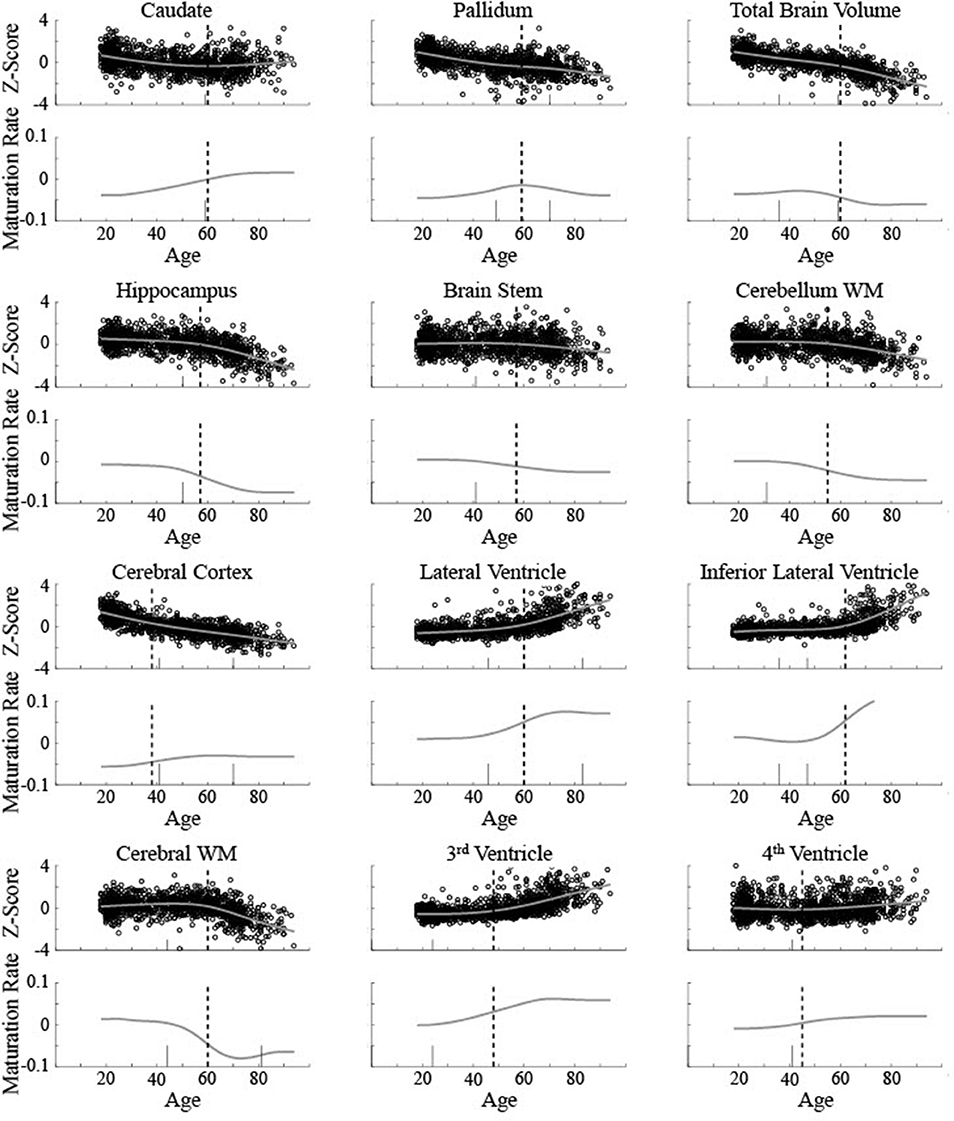
Figure 9. Biological data for 12 brain measurements (circles) is shown along with the smoothing spline curve fit (smooth line) for all measurements classified as non-linear curve types. Top rows show volume (z-score) and the bottom rows show the calculated instantaneous slope (maturation rate: $\dot{\text{y}}$) based on the smoothing spline fit. The upper left measurement (caudate nucleus) was classified as Curve Type 1, the upper middle (pallidum) was classified as Curve Type 2, with the remaining classified as Curve Type 3. Dotted vertical lines show the critical age guess based on the classification procedure. Short solid vertical lines show the critical ages reported in Fjell et al. [3].

FIGURE 10

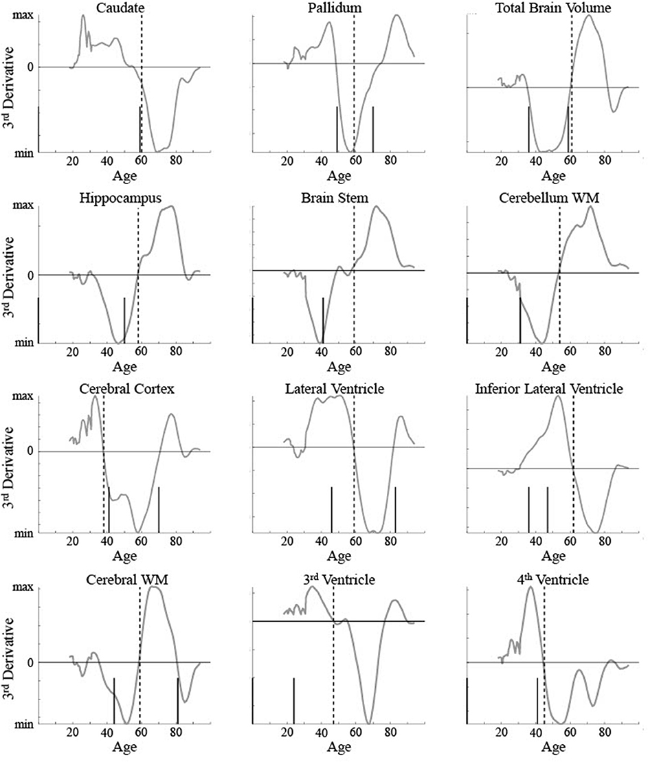
Figure 10. 3rd derivatives for 12 brain measurements (smooth line) are shown along with the determined critical ages (vertical lines) for all measurements classified as non-linear curve types. The upper left measurement (caudate nucleus) was classified as Curve Type 1, the upper middle (pallidum) was classified as Curve Type 2, with the remaining classified as Curve Type 3. Dotted vertical lines show the critical age guess based on the classification procedure. Short solid vertical lines show the critical ages reported in Fjell et al. [3].

Results of PCA Analysis

Principal Component Analyses (PCA) were performed on the low and realistic noise data sets to explore what differentiating information was present in the smoothing splines without using preconceived theoretical maturation patterns (Figure 11). The PCA output for the biological data was included for visual comparison with the simulated data though no statistics could be run on it since the curve types were not explicitly known. In general, the first two principal components for each type of input were sufficient to account for a majority of the variance across all examples with the greatest amount of variance accounted for by a low frequency differentiation between low and young ages. Significant differences between the curve types on particular principal components can help elucidate the information used by a classifier that categorizes curve type. Statistics were run on the first five components regardless of how much of the total variance was explained in order to give an adequate opportunity for the PCA results to differentiate between curve type.

FIGURE 11

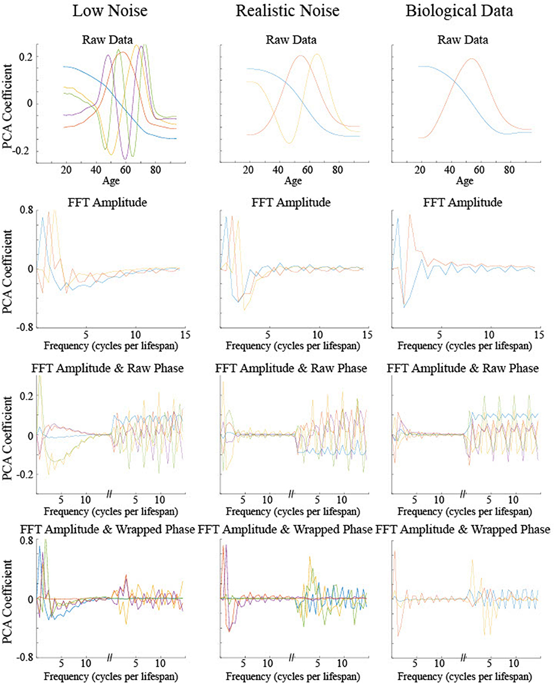
Figure 11. The principal components based on the PCA of four different input types for three different data sets. Only the set of components that accounted for at least 95% of the variance were included or the first five components are shown, whichever was the smaller number. The color of the components indicates the relative proportion of the variance explained by that component, in the following order from most to least: blue, red, orange, purple, and green.

For PCA on the raw data, i.e., maturation rate time course, no components demonstrated significant differences across curve type (all F's < 1.3, p's > 0.27), despite the first five components accounting for a large proportion of the variance (92% for low noise, 99% for realistic noise). For PCA on the power spectrum following FFT on the maturation rate time course, again no components demonstrated significant differences across curve type [most F's < 1, p's > 0.45, fifth low noise component F_{(3, 996)} = 2.26, p = 0.08, fourth realistic noise component F_{(3, 996)} = 2.64, p = 0.05], despite the first five components accounting for a large proportion of the variance (98% for low and realistic noise). For PCA on the power spectrum combined with the raw phase spectrum, similarly no components demonstrated significant differences across curve type (all F's < 1.1, p's > 0.37), despite the first five components accounting for a large proportion of the variance (73% for low noise, 85% for realistic noise).

For PCA on the power spectrum combined with the wrapped phase spectrum in order to remove discontinuities in the phase spectrum for adjacent frequencies, a different pattern emerged as some of the components were useful in differentiating curve type. For low noise data, though the first component, which accounted for 46% of the variance, did not show a significant difference between curve type [F_{(3, 996)} = 0.40, p = 0.76], each of the next three components, which together accounted for 45% of the variance, did show a significant difference between curve type (each F > 70, p < 0.001). The second component is relatively flat for the power spectrum but discriminates between a set of low frequency phases from higher frequency phases (see red curve in Figure 11). Tukey post hoc testing indicated that this component differentiated Curve Type 1 and Curve Type 2 from each other and the other curve types (p's < 0.001), but did not differentiate Curve Type 3 and Curve Type 0, i.e., the linear maturation pattern (p = 0.37). The third and fourth components had a similar shape in the power spectrum, differentiating relatively low frequencies from the lowest frequencies and medium frequencies, but had opposite shapes in the phase spectrum (see purple and orange curves in Figure 11). Tukey post hoc testing indicated that the third component differentiated Curve Type 3 and Curve Type 0 from each other and the other curve types (p's < 0.001), but did not differentiate Curve Type 1 and Curve Type 2 (p = 0.66) whereas the fourth component differentiated Curve Type 0 from the non-linear curve types (p's < 0.001), with a possible separation from Curve Type 1 and Curve Type 3 (p = 0.046). For PCA on the power spectrum combined with the wrapped phase spectrum using realistic noise data, again there was differentiating information to separate out the curve types. However, the components with significant differences across curve type were much more heavily weighted toward the phase spectrum information than the power spectrum (blue, orange, and green curves in Figure 11), with the opposite true for the components with no significant differences (red and purple curves in Figure 11). Specifically, the first component, which accounted for 65% of the variance, was shown through Tukey post hoc testing to differentiate Curve Type 0, the linear maturation pattern, from the three non-linear curve types (p's < 0.001) but not differentiate the other curves from one another (p's > 0.52). The third component, which accounted for 7% of the variance, differentiated all curve types (p's < 0.001) whereas the fifth component, which accounted for 1% of the variance, differentiated Curve Type 1 and Curve Type 2 from each other and the other curve types (p's < 0.001), but did not differentiate Curve Type 3 and Curve Type 0 (p = 0.72).

Discussion

Smoothing splines were shown to be a valid means of identifying a set of maturation patterns for adult ages and shown to contain the essential information required to determine a single critical age for the patterns. However, zero points of any particular derivative were not sufficient to determine the critical age when maturation patterns contain critical ages defined by different derivative zero points, arguing against using third derivative zero points to determine critical ages for all maturation patterns. Classifying the type of maturation pattern prior to determining the critical age resulted in identified critical ages within 5 years of the actual critical age for a vast majority of trials, even for realistic noise levels. The results of PCA on various types of input (maturation time course, FFT of the maturation time course including the power and phase spectra), demonstrated that only when appropriate phase information is included can the curve types be differentiated, clarifying why linear classifiers performed much worse than non-linear classifiers. The method presented here holds promise for differentiating the maturation patterns of individual brain areas to identify both the type of developmental pattern occurring and the critical age that represents the key reflection point of that pattern.

In addition to determining a validated method for identifying critical ages in brain maturation, a goal of this study was to rule out other methods by elucidating deficiencies in using limited sources of information. As such, any methods seeking to rely solely on the 1st and 2nd derivative zero points or principal components of the maturation patterns were found to be insufficient. Of special interest was assessing the effectiveness of using 3rd derivative zero points as that method had previously been used [3, 6, 8]. That method was found to work well for most brain measurements as a vast majority of those tested here were determined to have an accelerating non-linearity as their developmental maturation pattern. Still, the method is invalid for the minority of brain areas with a U-shaped maturation pattern (Curve Type 1) and systematically misrepresents the critical age of development for sigmoidal maturation patterns (Curve Type 2). In regards to the identified critical ages for areas with clear changes in the maturation rate, the 3rd derivative zero point generally corresponds to age ranges with clear visual bends in their observed sizes (see the rows of z-scores in Figure 9). Such age ranges may possibly be of clinical relevance if they also indicate a deviation from maturation across younger ages. However, caution should be exercised when interpreting the 3rd derivative zero points for sigmoidal maturation patterns (Curve Type 2) as their proximity to the reflection point for the true maturation pattern is highly impacted by noise in the observed data (see Figure 3).

One potential issue identified here with using 3rd derivative zero points to identify critical ages in development is the high number of zero points found for data simulated based on a ground truth curve with only a single zero point. This brings up two main issues—how to determine which zero point to use to identify a single critical age and how to determine if it is appropriate to identify more than one critical age of development over the lifespan. The current method proposed above took into account the magnitude of the peak or trough of the 2nd derivative. This is equivalent to identifying the 3rd derivative zero point with the greatest local slope. Based on 3rd derivatives shown in Figure 10 for biological data, most brain areas had a single zero point with a steep slope, justifying this choice. However, some areas, such as the cerebral cortex and cerebral white matter, show two zero points with similar magnitude slopes. A different selection method may have chosen the older value as the critical age. There is some evidence, seen in Figure 8, that the current method may be biased toward choosing the younger of two zero points when the actual critical age is over 70. Performance of the method as a function of age when there is a non-uniform distribution of observations across age could be examined further in a follow up study. Identifying maturational patterns with multiple critical ages is a limitation of the current method and is further discussed below.

Here simulated data was used to validate procedures that were then used on previously published data. Validation on simulated data is an essential step in that it verifies the performance of the method but using it on real data demonstrates that the method is actually applicable. Basing simulations on biologically constrained variables can assist in identifying limitations of conclusions drawn from analysis of observed data. For instance, the simulated data with an experimentally observed age distribution highlighted particular issues in determining critical ages above 70 that were not present with uniformly distributed ages, especially for Curve Type 1. This was likely due to having a sparser sampling of the population in the oldest age groups. The increase in availability of open-access data facilitates the process of testing new procedures on large samples of real data [21]. Prior studies have used ground truth simulations before applying analysis methods of MRI data to clinical assessments in order to explore the effects of sampling procedures and individual differences in trajectories (e.g., [22]). Predicted brain age is a method that uses the ground truth of someone's actual age to infer a different biological age as an indicator for health markers with deviations from a normative maturation pattern possibly occurring as a result of environmental factors [23]. Similar to what was done here, machine learning is first used to identify patterns present in the data but predicting brain age utilizes a continuous output value, i.e., age, whereas here a limited number of maturation patterns are distinguished between so that a continuous output value, i.e., critical age, can then be extracted. Better understanding of the critical ages in brain maturation could help in determining brain age or the qualitative differences in health that may exist before and after such a critical age.

Three maturation patterns were emphasized because they were found previously in the literature (see “Introduction”) and correspond to typical developmental processes. The linear change in maturation rate of Curve Type 1 would represent, in its inverted U-shaped form, sustained neuronal growth followed by sustained loss, which would be consistent with a combination of two different developmental processes acting at different points in the lifespan. The Gaussian shaped maturation pattern of Curve Type 2 would represent growth or loss at isolated times in the lifespan, such as puberty. The sigmoidal maturation pattern of Curve Type 3 is consistent with acceleration due to normal aging or disease progression. It is quite likely that various neurobiological processes acting at different points along the lifespan can result in other less-well defined brain maturation patterns ([3, 7]—see Figure 4, p. 2245; [23, 24]) or that other types of patterns would be revealed when younger ages are included [15, 25]. The classification scheme presented here would not detect multiple critical ages. In principle the method could be extended to determine that multiple critical ages are present and furthermore which component of the maturation rate would be most informative for determining each of them. However, the specific formulation of such a process is outside the scope of the current study. Though much of the early studies on how brain areas change in size over the lifespan utilized cross-sectional data, there has been an increase in the number of studies using longitudinal data collection. One caution on relying on estimates based on cross-sectional data alone is the variability added due to differences in scanner properties and the sex of the subjects [26, 27]. Though the current analysis focused on cross-sectional data, there has been good consistency found in the estimated rate of change when cross-sectional data was compared to longitudinal data in older adults ([3, 14] though see [28]). While it is an open empirical question regarding whether the same critical ages would be identified using either type of data, consistency in the results is expected if the general shapes of the maturation patterns match. Furthermore, longitudinal data could be used as the basis of the maturation pattern as opposed to a non-parametric estimation based on changes in volume across age since estimates of brain volume loss are reliable [14, 29]. With that said, additional benefits may be gained in regards to clinical assessment if an individual is described based on their deviation from the mean maturation pattern [30] or when the age trajectories of individuals are determined beyond the group-based maturation pattern [8].

Some limitations of the method described here may be noted. The critical age is based on a mathematical approximation of the underlying function but may not correspond to when a change first appears in the population, as evidenced by the location of the dotted vertical lines along the growth curves shown in Figure 9. Identifying initial changes in maturation rate requires pulling additional information from the smoothing spline. This would be possible using a sliding window that defines the expected trajectory of maturation rate based on a preceding age range that could signal discontinuities in the trajectory. A smoothing spline fit would not be required for such an analysis as Schippling et al. [9], used a non-parametric technique with smaller windows applied to various points along the lifespan with the emphasis on determining the maturation rate but not critical ages. Other approaches may be more appropriate in determining when different populations diverge from one another [13]. Another issue is that only a single critical age is being identified when it is possible that more than one may exist, especially when the entire lifespan is included as opposed to just adult ages. Using more complex maturation patterns based on the combination of different patterns described here would still allow for using the principle of classifying the pattern followed by extracting multiple critical ages based on derivative zero points.

Data Availability Statement

The code used in this study can be found in the Mendeley Dataset Repository (http://dx.doi.org/10.17632/2pkhbdgjys.2).

Author Contributions

DN contributed to all aspects of the project and writing.

Conflict of Interest

The author declares that the research was conducted in the absence of any commercial or financial relationships that could be construed as a potential conflict of interest.

References

1. Walhovd KB, Westlye LT, Amlien I, Espeseth T, Reinvang I, Raz N, et al. Consistent neuroanatomical age-related volume differences across multiple samples. Neurobiol Aging. (2011) 32:916–32. doi: 10.1016/j.neurobiolaging.2009.05.013

PubMed Abstract | CrossRef Full Text | Google Scholar

2. Zeigler G, Dahnke R, Jäncke L, Yotter RA, May A, Gaser C. Brain structural trajectories over the adult lifespan. Hum Brain Mapp. (2012) 33:2377–89. doi: 10.1002/hbm.21374

PubMed Abstract | CrossRef Full Text | Google Scholar

3. Fjell AM, Weslye LT, Grydeland H, Amlien I, Espeseth T, Reinvang I, et al. Critical ages in the life course of the adult brain: nonlinear subcortical aging. Neurobiol Aging. (2013) 34:2239–47. doi: 10.1016/j.neurobiolaging.2013.04.006

PubMed Abstract | CrossRef Full Text | Google Scholar

4. Good CD, Johnsrude IS, Ashburner J, Henson RNA, Friston K, Frackowiak RSJ. A voxel-based morphometric study of ageing in 465 normal adult human brains. Neuroimage. (2001) 14:21–36. doi: 10.1006/nimg.2001.0786

PubMed Abstract | CrossRef Full Text | Google Scholar

5. Walhovd KB, Fjell AM, Reinvang I, Lundervold A, Dale AM, Eilertsen DE, et al. Effects of age on volumes of cortex, white matter and subcortical structures. Neurobiol Aging. (2005) 26:1261–70. doi: 10.1016/j.neurobiolaging.2005.05.020

PubMed Abstract | CrossRef Full Text | Google Scholar

6. Fjell AM, Walhovd KB, Westlye LT, Østby Y, Tamnes CK, Jernigan TL, et al. When does brain aging accelerate? Dangers of quadratic fits in cross-sectional studies. Neuroimage. (2010) 50:1376–83. doi: 10.1016/j.neuroimage.2010.01.061

PubMed Abstract | CrossRef Full Text | Google Scholar

7. Raz N, Rodrigue KM. Differential aging of the brain: patterns, cognitive correlates and modifiers. Neurosci Biobehav R. (2006) 30:730–48. doi: 10.1016/j.neubiorev.2006.07.001

PubMed Abstract | CrossRef Full Text | Google Scholar

8. Zeigler G, Dahnke R, Gaser C. Models of the aging brain structure and individual decline. Front Neuroinform. (2012) 6:3. doi: 10.3389/fninf.2012.00003

PubMed Abstract | CrossRef Full Text | Google Scholar

9. Schippling S, Ostwaldt A-C, Suppa P, Spies L, Manogaran P, Gocke C, et al. Global and regional annual brain volume loss rates in physiological aging. J Neurol. (2017) 264:520–8. doi: 10.1007/s00415-016-8374-y

PubMed Abstract | CrossRef Full Text | Google Scholar

10. Wilkinson DJ. Stochastic modelling for quantitative description of heterogeneous biological systems. Nature Rev Genet. (2009) 10:122–33. doi: 10.1038/nrg2509

PubMed Abstract | CrossRef Full Text | Google Scholar

11. Székely T, Burrage K. Stochastic simulation in systems biology. Comput Struct Biotechnol J. (2014) 12:14–25. doi: 10.1016/j.csbj.2014.10.003

PubMed Abstract | CrossRef Full Text | Google Scholar

12. Ghirardi O, Cozzolino R, Guaraldi D, Giuliani A. Within- and between-strain variability in longevity of inbred and outbred rats under the same environmental conditions. Exp Gerontol. (1995) 30:485–94. doi: 10.1016/0531-5565(95)00002-X

PubMed Abstract | CrossRef Full Text | Google Scholar

13. Pagani M, Giuliani A, Öberg J, Chincarini A, Morbelli S, Brugnolo A, et al. Predicting the transition from normal aging to Alzheimer's disease: a stastical mechanistic evaluation of FDG-PET data. Neuroimage. (2016) 141:282–90. doi: 10.1016/j.neuroimage.2016.07.043

PubMed Abstract | CrossRef Full Text | Google Scholar

14. Crivello F, Tzourio-Mazoyer N, Tzourie C, Mazoyer B. Longitudinal assessment of global and regional rate of grey matter atrophy in 1,172 healthy older adults: modulation by sex and age. PLoS ONE. (2014) 9:e114478. doi: 10.1371/journal.pone.0114478

PubMed Abstract | CrossRef Full Text | Google Scholar

15. Coupé P, Catheline G, Lanuza E, Manjón JM. Towards a unified analysis of brain maturation and aging across the entire lifespan: a MRI analysis. Hum Brain Mapp. (2017) 38:5501–18. doi: 10.1002/hbm.23743

PubMed Abstract | CrossRef Full Text | Google Scholar

16. Pfefferbaum A, Rohlfing T, Rosenbloom MJ, Chu W, Colrain IM, Sullivan EV. Variation in longitudinal trajectories of regional brain volumes of healthy mean and women (ages 10 to 85 years) measured with atlas-based parcellation of MRI. Neuroimage. (2013) 65:176–93. doi: 10.1016/j.neuroimage.2012.10.008

PubMed Abstract | CrossRef Full Text | Google Scholar

17. Christianini N, Shawe-Taylor J. An Introduction to Support Vector Machines and Other Kernel-Based Learning Methods. Cambridge: Cambridge University Press (2000).

Google Scholar

18. Hastie T, Tibshirani R, Friedman J. The Elements of Statistical Learning, 2nd ed. New York, NY: Springer (2009).

Google Scholar

19. Bender R, Lange S. Adjusting for multiple testing – when and how? J Clin Epidemiol. (2001) 54:343–9. doi: 10.1016/S0895-4356(00)00314-0

PubMed Abstract | CrossRef Full Text | Google Scholar

20. Thornhill NF, Shah SL, Huang B, Vishnubhotla A. Spectral principal component analysis of dynamic process data. Control Eng Pract. (2002) 10:833–46. doi: 10.1016/S0967-0661(02)00035-7

CrossRef Full Text | Google Scholar

21. Madan CR. Advances in studying brain morphology: the benefits of open-access data. Front Hum Neurosci. (2017) 11:405. doi: 10.3389/fnhum.2017.00405

PubMed Abstract | CrossRef Full Text | Google Scholar

22. Zeigler G, Ridgway GR, Dahnke R, Gaser C. Individualized Guassian process-based prediction and detection of local and global gray matter abnormalities in elderly subjects. Neuroimage. (2014) 97:333–48. doi: 10.1016/j.neuroimage.2014.04.018

PubMed Abstract | CrossRef Full Text | Google Scholar

23. Cole JH, Franke K. Predicting age using neuroimaging: innovative brain ageing biomarkers. Trends Neurosci. (2017) 40:681–90. doi: 10.1016/j.tins.2017.10.001

PubMed Abstract | CrossRef Full Text | Google Scholar

24. Vinke EJ, de Groot M, Venkatraghavan V, Klein S, Niessen WJ, Ikram MA, et al. Trajectories of imaging markers in brain aging: the Rotterdam Study. Neurobiol Aging. (2018) 71:32–40. doi: 10.1016/j.neurobiolaging.2018.07.001

PubMed Abstract | CrossRef Full Text | Google Scholar

25. Tamnes CK, Østby Y, Fjell AM, Westlye LT, Due-Tønnessen P, Walhovd KB. Brain maturation in adolescence and young adulthood: regional age-related changes in cortical thickness and white matter volume and microstructure. Cereb Cortex. (2010) 20:534–48. doi: 10.1093/cercor/bhp118

PubMed Abstract | CrossRef Full Text | Google Scholar

26. Potvin O, Dieumegarde L, Duchesne S. Normative morphometric data for cerebral cortical areas over the lifetime of the adult human brain. Neuroimage. (2017) 156:315–39. doi: 10.1016/j.neuroimage.2017.05.019

PubMed Abstract | CrossRef Full Text | Google Scholar

27. Ma D, Popuri K, Bhalla M, Sangha O, Lu D, Cao J, et al. Quantitative assessment of field strength, total intracranial volume, sex, and age effects on the goodness of harmonization for volumetric analysis on the ADNI database. Hum Brain Mapp. (2018) 40:1507–27. doi: 10.1002/hbm.24463

PubMed Abstract | CrossRef Full Text | Google Scholar

28. Pfefferbaum A, Sullivan EV. Cross-sectional versus longitudinal estimates of age-related changes in the adult brain: overlaps and discrepancies. Neurobiol Aging. (2015) 36:2563–7. doi: 10.1016/j.neurobiolaging.2015.05.005

PubMed Abstract | CrossRef Full Text | Google Scholar

29. Opfer R, Ostwaldt A-C, Walker-Egger C, Manogaran P, Sormani MP, De Stefano N, et al. Within-patient fluctuation of brain volume estimates from short-term repeated MRI measurements using SIENA/FSL. J Neurol. (2018) 265:1158–65. doi: 10.1007/s00415-018-8825-8

PubMed Abstract | CrossRef Full Text | Google Scholar

30. Dickie DA, Job DE, Gonzalez DR, Shenkin SD, Ahearn TS, Murray AD, et al. Variance in brain volume with advancing age: implications for defining the limits of normality. PLoS ONE. (2013) 8:e84093. doi: 10.1371/journal.pone.0084093

PubMed Abstract | CrossRef Full Text | Google Scholar