Modeling the Spread of COVID-19 in Lebanon: A Bayesian Perspective

Introduction

As the Coronavirus Disease 2019 (COVID-19) pandemic progresses, countries around the world, including Lebanon, are increasingly implementing a range of responses that are intended to help prevent the transmission of this disease. Until a COVID-19 vaccine becomes available, strict measures from closing schools and universities to locking down entire cities and countries were enforced to suppress the virus transmission, thereby, slowing down the growth rate of cases and rapidly reducing case incidence.

Structured mathematical and statistical techniques can be potentially powerful tools in the fight against the COVID-19 pandemic. These techniques allow the COVID-19 transmission to be modeled, so the resulting models can be used to predict and explain COVID-19 infections. This may be of great usefulness for health care decision-makers, as it gives them the time to intervene on the local public health systems, thereby take the appropriate actions to contain the spreading of the virus to the degree possible. A statistical model that describes the spread of the disease over time is, therefore, essential to this endeavor. Since the outbreak of the pandemic, there has been a scramble to use and explore various statistical techniques, and other data analytic tools, for these purposes.

Advancement in statistical modeling, such as Bayesian inference methods facilitates the analysis of contagion occurrence through time. It is well-documented that infectious diseases grow exponentially and are usually driven by the basic reproduction number R (see for example [1]) for a given population. The value of R is defined as the ratio between consecutive new occurrences of infection. This describes a short-term dependence. However, according to [2] for the case of COVID-19, incubation time varies substantially among individuals and incidence and so measurement may not be uniform across different populations, thereby a long-term dependence should be induced. This implies that, a model that describes the contagion dynamics of COVID-19 should ideally contain both short-term and long-term components as determining factors of newly infected counts. Such a model is hugely important to understand whether the contagion of the virus has a trend (upward or downward) and where exactly each country stands on that trend. This can provide support to decision-makers involved in contrasting the spread of the COVID-19 to perceive the effectiveness of their policy measures against the virus and what their future steps should be.

We aim in the presenting paper to model and predict the number of COVID-19 infections in Lebanon using Bayesian methods. To this aim, we propose two different models of increasing complexity using Bayesian Markov chain Monte Carlo (MCMC) simulation methods. These models include Poisson autoregressive as a function of a short-term dependence only and Poisson autoregressive as a function of both a short-term dependence and a long-term dependence. The Poisson autoregressive model that includes both short-term and long-term memory components performs best in terms of mean predictions, root mean squared error (RMSE), and deviance information criterion (DIC). A model of this kind, while mathematically expressing the current practices in the modeling on the global spread of COVID-19, produces findings that could be beneficial for policy decision-makers. Our contribution in the present study is a Bayesian statistical model for the spread of COVID-19 which, by accounting for dependence between infection counts, can better detect the contagion curve dynamics, so can shed some light on the understanding of its possible future path. The Bayesian model is also flexible in characterizing inputs to regression models and more comprehensive in characterizing the uncertainty in the model outputs.

To our knowledge, this study would be the first in the Middle East to analyze and predict the spread of COVID-19 using Bayesian methods and, therefore, neighboring countries would benefit from this study along with the model until similar studies are conducted in the region.

Methods

Data Source

The Ministry of Public Health has started to release a daily bulletin about COVID-19 infections in Lebanon since 23 February 2020. Data are available from the website of the Ministry of Public Health (MoPH) [3] and worldometer website [4]. The overall temporal distribution of daily counts of COVID-19 cases (blue line) is presented in Figure 1. The data covers the period from February 23 to April 18, 2020. The plot indicates that COVID-19 contagion in Lebanon has achieved a complete cycle. Specifically, Figure 1 shows an upward trend until a peak is reached on March 23 and after this date, a decreasing trend is then observed.

FIGURE 1

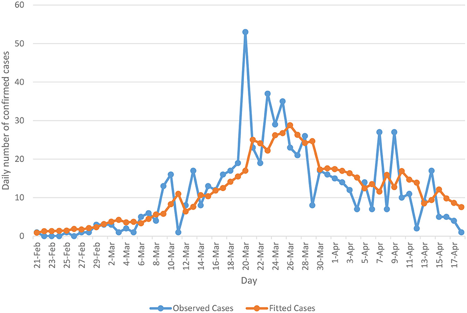
Figure 1. Actual (blue line) and fitted (orange line) cases based on the Poisson autoregressive model (Model 2).

Bayesian Methods

Bayesian methods allow the use of information other than the study data, into the analysis [5]. Such information is represented as a prior distribution and is combined with the likelihood function to give a posterior distribution on which inferences are subsequently made. In Bayesian analysis, the use of subjective/informative a priori beliefs is not a necessity as “vague” priors can be utilized. Given the focus in the present study is not the incorporation of prior information, all prior distributions that will be used for model parameters are considered to be “vague.” However, in order to examine the robustness of our results under different prior probability distributions, sensitivity analysis is performed. We consider this finding in more detail in the discussion section.

MCMC Methods

Bayesian methods rest upon the computation of the posterior distributions for model parameters. MCMC methods [6] are computer-intensive methods that would allow user to draw samples from the posterior distribution, without the need to explicitly compute the posterior distribution. Each model in this study will be fit using the software package WinBUGS [7] and the relevant WinBUGS code is provided in the Appendix.

Model Development

Two different models were fitted to the data as follows:

1. Poisson autoregressive as a function of a short-term dependence only

2. Poisson autoregressive as a function of both a short-term dependence and a long-term dependence

Following Agosto and Giudici [2], the number of new cases y_t reported at time (day) t is assumed to follow a Poisson distribution i.e.,

$\begin{array}{l}{y}_t~Poisson({\lambda }_t),\end{array}$

with a log-linear autoregressive intensity specification, as follows:

$\begin{array}{l}\text{log }({\text{λ}}_{\text{t}})=\alpha +\beta \text{ log}(1+y_{\text{t }-1})(\text{Model }1)\\ \text{log}({\text{λ}}_{\text{t}})=\alpha +\beta \text{ log}(1+y_{\text{t}-1})+\gamma \text{ log}({\lambda }_{\text{t}-1})(\text{Model }2)\end{array}$

In each model, the inclusion of 1 in log (1 + y_t−1) allows to address the problem generated by zero values, α represents the intercept term and β expresses the short-term dependence of the expected number of cases reported at time t, λ_t, on these observed in the previous day (time t−1). The γ component in model 2 corresponds to a trend component and, more specifically, it represents the long-term dependence of λ_t on all past counts of the observed process. Note that the use of a log-linear autoregressive intensity specification, rather than linear, allows for negative dependence. Inference for this model was conducted via the Maximum Likelihood estimation method in Agosto and Giudici [2].

Model Estimation

Both models were implemented from a Bayesian perspective using Gibbs sampling MCMC simulation methods using WinBUGS software [7]. The relevant code to undertake the Bayesian models is given in the Appendix. For every model, an initial 10,000 iterations were run as a “burn-in” to reach convergence. To assess convergence, two parallel chains were started from different initial values, and the ratio of the within-chain to between-chain variance was then monitored and converged at about one, indicating convergence had been reached [8]. The initial run was then followed by an additional 50,000 iterations for parameter estimation purposes. To this end, the prior distributions for all the regression parameters (α, β, and γ) were specified as

$\begin{array}{l}\alpha ,\beta ,\gamma ~\text{ N}(0,10^6).\end{array}$

That is, centered at zero with a large variance so as to be relatively non-informative.

Model Validation

The two models were compared in terms of their coefficients with their associated 95% credible intervals (CI), as well as their predictive performance using plots of predicted to actual values, calculations of the mean predictions, RMSE and DIC. The RMSE criterion for the mean is defined as:

$\begin{array}{l}RMSE={\left(\frac{{\displaystyle {\sum }_{t=1}^T}{(y_t-{ŷ}_t)}^2}{T}\right)}^{1/2}\end{array}$

where y_t is the observed value of new infections reported at time (day) t, ŷ_t is the fitted value and T is the number of time points in the sample. In addition, the DIC, which combines measures of both model fit and model complexity, is defined by

$\begin{array}{l}DIC=\overline{D}+P_D\end{array}$

where $\overline{D}$ represents the posterior mean deviance and P_D is the effective number of parameters representing model complexity. The minimum DIC denotes the model best fitting the data [9].

Results

Model Estimation and Validation

Table 1 shows the estimated autoregressive coefficients for both models together with their associated 95% CI. We notice that all coefficients had the expected positive sign as well as their credible intervals excluding zero, indicating the presence of a short-term dependence for model 1 and both a short-term dependence and a long-term trend for model 2. A testing of the models' performance is also shown in Table 1, where model 2 was found to perform best by scoring the best RMSE and DIC with 7.68 and 444.7, respectively, in comparison to model 1 (RMSE = 8.56, DIC = 517.5).

TABLE 1

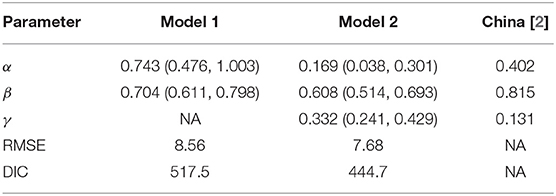
Table 1. Model coefficients and model performance.

Model Predictions

Model 2 has been tested in terms of its predictive ability where the resulting fitted mean occurrences (orange line) have been plotted along with the actual occurrences (blue line) in Figure 1. As can be seen from the plot, the Poisson autoregressive model as a function of both a short-term dependence and a long-term dependence predicts the data quite well. With aim of better interpreting the short-term time series and long-term time series of model 2, we notice from Table 1 that the estimated γ parameter is lower than β, confirming that a downward trend data is accumulated. Additionally, we split the Lebanese data into two time periods and we separately fit the model for each data set. More specifically, we first fit the model on the data, which covers the period from February 23 to March 23, 2020 and then on the data from March 24 onwards. Analysis from the first data set revealed that γ was larger than β, confirming the presence of an upward trend (the γ component) which absorbs the short-term component. After this date, the estimated γ parameter became lower, so a downward trend data is accumulated.

Agosto and Giudici [2] drew a similar conclusion from their analysis of the Chinese data, which covers the period from January 20 to March 15, 2020. Their estimated β and γ parameters (final column of Table 1) revealed that the contagion cycle was in a downward trend (γ < β). On the other side, their analysis for South Korea revealed non-significant estimate for the estimated γ parameter, confirming absence of a trend effect on the daily cases. However, for Italy, their results showed that the estimated β parameter was smaller than γ, suggesting that the trend of the contagion has not peaked yet.

Uncertainty in Model Predictions

A key potential advantage of the Bayesian approach is that it produces estimates of the uncertainty in the number of new infections predictions from the model. The classical models, like [2], produce data on the uncertainty in the model parameters, however, they do not produce estimates of the uncertainty in the number of new infections predictions from the model. Figure 2 shows the probability distributions for the last four daily count predictions (λ₅₅–λ₅₈) from the model. From these distributions, the mean, median, standard deviation, and corresponding 95% credible intervals along with Monte Carlo (MC) error can be computed. The distributional statistics for all daily counts predictions from the model are reported in Table 2. These results show that Bayesian method is more flexible in characterizing inputs to regression models and more comprehensive in characterizing the uncertainty in the model outputs.

FIGURE 2

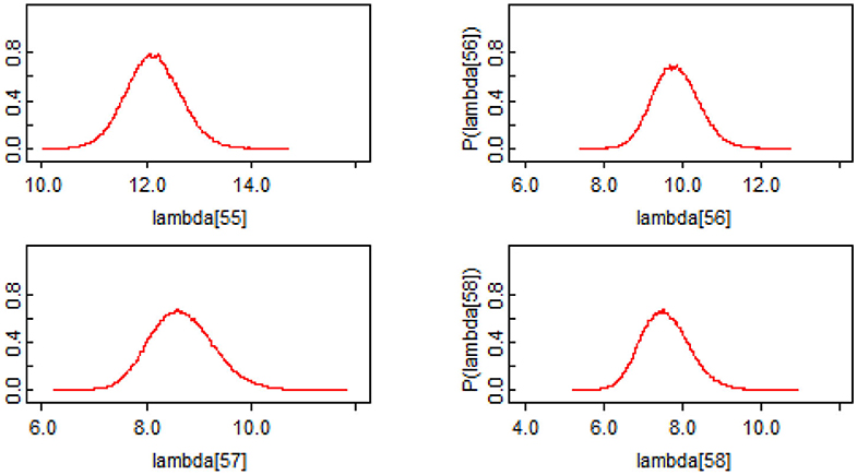
Figure 2. Example Probability Distributions for the last four daily counts predictions of COVID-19 cases [55–58th case predictions in Table 2 (i.e., λ₅₅−λ₅₈)].

TABLE 2

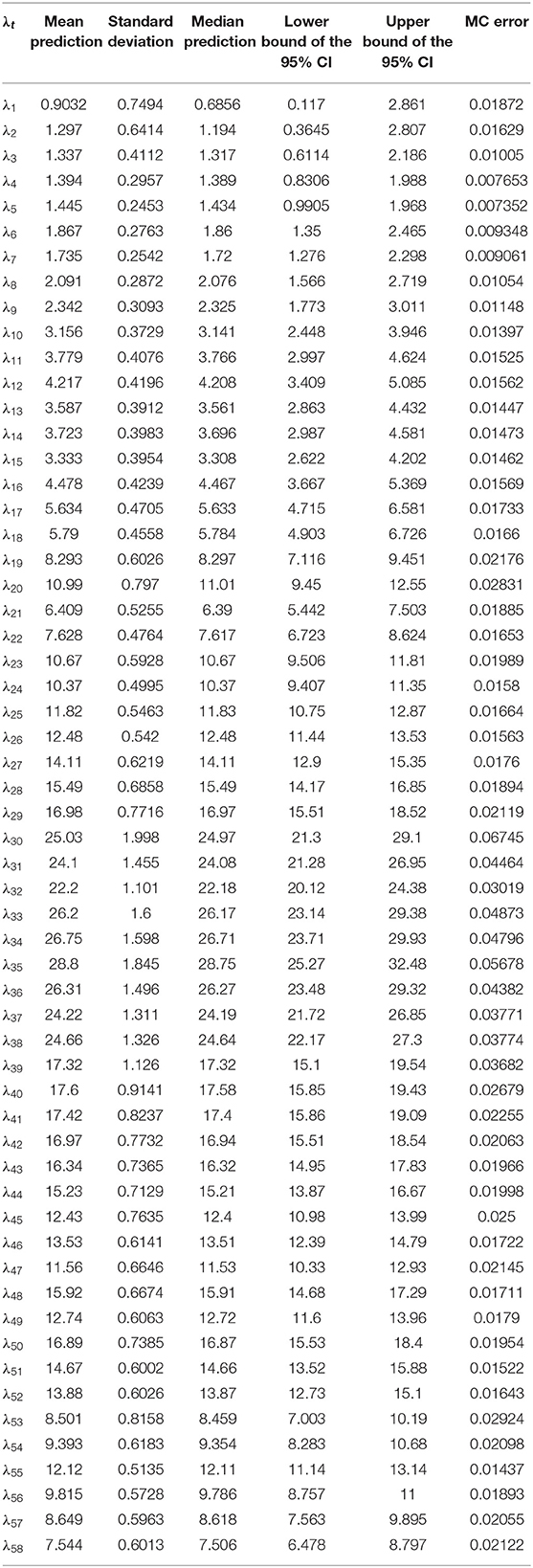
Table 2. Characteristics of distributions for the daily counts predictions.

Discussion

In this article, we have analyzed, by modeling, the trend of the current COVID-19 pandemic in Lebanon along time. We have developed two different models of increasing complexity using Bayesian MCMC simulation methods, and found that the Poisson autoregressive as a function of both a short-term dependence and a long-term dependence provides the best fit to the data. The use of Poisson autoregressive model that allows to capture short and long term memory effects can greatly improve the estimation of number of new cases and can indicate whether disease has an upward/downward trend, and where about every country is on that trend, all of which can help the public decision-makers to better plan health policy interventions and take the appropriate actions to contain the spreading of the virus to the degree possible.

Through employing Bayesian methods, we were able to incorporate parameter estimation uncertainty in our results. In particular, they allow to provide information on the predictive performance precision as a direct output from the modeling process, and this in turn can be used to prepare credible intervals for posterior distributions. For example, posterior distributions constructed in Bayesian analysis permit inference of functions of parameters (e.g., tail probabilities of parameters), which the classical analysis, like [2], cannot do.

Model findings are presented for the actual time series of Lebanon, but can be easily reproduced and extended to other countries and more time periods as more data becomes available. Ongoing research on conducting the proposed methodology for the US, UK, China, Italy, and South Korea has preliminary results that are very promising. The model can also be used to monitor the spread of the virus in the post-lockdown phase, which in turn would enable a comparative analysis of the effectiveness of alternative policy measures. Further research is also underway to assess this. It is perhaps worth mentioning that the model proposed must be analyzed with a caveat in mind related to the fact that the dataset still covers a relatively limited timeframe.

To this end, a key note related to the prior distributions that are put on the model parameters: Although these prior distributions were considered to be non-informative, it is recommended to perform sensitivity analysis to assess the impact of these distributions. Had said, for every regression parameter in the model, the mean for the normal prior distribution was varied from −50 to 50. The variance for the normal prior distributions was also varied from 10² to 10⁶. The posterior distributions for the regression parameters were found to change only minimally, thus a normal prior with variance 10⁶ is suitably non-informative and works generally well with our dataset. This implies that, for our model, results were robust over this array of prior distributions. More discussions regarding the choice of prior distributions are available in Spiegelhalter et al. [10].

Data Availability Statement

Publicly available datasets were analyzed in this study. Data are available from the website of the Ministry of Public Health in Lebanon on https://www.moph.gov.lb/en/Pages/2/24870/novel-coronavirus-2019.

Author Contributions

SK: conceptualization, formal analysis, methodology, software, validation, writing—original draft, writing—review, and editing.

Conflict of Interest

The author declares that the research was conducted in the absence of any commercial or financial relationships that could be construed as a potential conflict of interest.

References

1. Biggersta M, Cauchemez S, Reed C, Gambhir M. Finelli L. Estimates of the reproduction number for seasonal, pandemic, and zoonotic influenza: a systematic review of the literature. BMC Infect Dis. (2014) 14:480. doi: 10.1186/1471-2334-14-480

PubMed Abstract | CrossRef Full Text | Google Scholar

2. Agosto A, Giudici P. A poisson autoregressive model to understand COVID-19 contagion dynamics. Risks. (2020) 8:77. doi: 10.2139/ssrn.3551626

CrossRef Full Text | Google Scholar

3. Ministry of Public Health. Novel Coronavirus 2019. (2020). Available online at: https://www.moph.gov.lb/en/Pages/2/24870/novel-coronavirus-2019- (accessed April 19, 2020).

Google Scholar

4. Worldometer. Coronavirus Cases. (2020). Available online at: https://doi.org/10.1101/2020.01.23.20018549V2 (accessed April 19, 2020).

5. Gelman A, Carlin JB, Stern HS, Rubin DB. Bayesian Data Analysis. London: Chapman and Hall (1995). doi: 10.1201/9780429258411

CrossRef Full Text | Google Scholar

6. Gilks WR, Richardson S, Spiegelhalter DJ. Markov Chain Monte Carlo in practice. London: Chapman and Hall (1996). doi: 10.1201/b14835

CrossRef Full Text | Google Scholar

7. Spiegelhatler DJ, Thomas A, Best NG, Lunn D. WinBUGS User manual: Version 1.4. Cambridge: MRC Biostatistics Unit (2003).

Google Scholar

8. Gelman A, Rubin DB. Inference from iterative simulation using multiple sequences. Statistical Sci. (1992) 7:457–72. doi: 10.1214/ss/1177011136

CrossRef Full Text | Google Scholar

9. Spiegelhalter DJ, Best NG, Carlin BP, van der Linde A. Bayesian measures of model complexity and fit. J Royal Statistical Soc Ser B. (2002) 64:583–639. doi: 10.1111/1467-9868.00353

CrossRef Full Text | Google Scholar

10. Spiegelhalter DJ, Myles JP, Jones DR, Abrams KR. Bayesian methods in health technology assessment: a review. Health Technology Assessment. (2000) 4:4380. doi: 10.3310/hta4380

PubMed Abstract | CrossRef Full Text | Google Scholar

Appendix

WinBUGS Code—Bayesian Analysis of Poisson Autoregressive Model (Model 2)

model{

  # AR(1) model

  log(lambda [1]) <- w + alpha^*log(1+y0) + beta^*log(lambda0)

  y[1] ~ dpois(lambda [1])

  for(t in 2:N) {

  log(lambda[t]) <- w + alpha^*log(1+y[t-1]) + beta^*log(lambda[t-1])

  y[t] ~ dpois(lambda[t])

  }

  # Prior distribution

  w ~ dnorm(0.0, 1.0E-6)

  alpha ~ dnorm(0.0, 1.0E-6)

  beta ~ dnorm(0.0, 1.0E-6)

  y0 ~ dunif(0.001,1000)

  lambda0 ~ dunif(0.001,1000)

  }