Divergence of the Ensemble Transform Kalman Filter (LETKF) by Nonlocal Observations

1. Introduction

Data assimilation (DA) merges models and observations to gain optimal model state estimates. It is well-established in meteorology [1], geophysics [2], and attracts attention in life sciences [3]. Typical applications of DA serve to estimate model parameters [4] or provide initial conditions for forecasts [5]. A prominent technique is the ensemble Kalman filter [6], which allows to assimilate observations in nonlinear models. When underlying models are high-dimensional, such as in geophysics or meteorology, spurious correlations in forecast errors are detrimental to state estimates. A prominent approach to avoid this effect is localization of error covariances. The Local Ensemble Transform Kalman Filter (LETKF) [7] utilizes a localization scheme in observation space that is computationally effective and applicable to high-dimensional model systems. The LETKF applies to local observations [8] measured in the physical system under study, e.g., by radiosondes, and nonlocal observations measured over a large area of the system by, e.g., weather radar or satellites [9–11]. Since nonlocal observations represent spatial integrals of activity, and the localization scheme of the LETKF requests a single spatial location of each observation, it is conceptually difficult to apply the LETKF to nonlocal observations. In fact, present localization definitions [10, 12] of nonlocal observations attempt to estimate the best single spatial location neglecting the spatial distribution of possible activity sources. A recent study [13] on satellite data assimilation proposes to choose the localization radius equal to the spatial distribution width of radiation sources. This spatial source distribution is the sensitivity function of the nonlocal observation and is part of the model system. The present work considers the hypothesis that the relation between localization radius and sensitivity function width plays an important role in the filter performance.

Merging the model forecast state and observations, the ensemble Kalman filter tears the analysis, i.e., the newly estimated state, toward the model forecast state and thus underestimates the forecast error covariance matrix due to a limited ensemble size [14]. This is enforced by model errors [15, 16] and leads to filter divergence. Moreover, if the forecast error covariances are too large, the forecasts have too less weight in the assimilation step and the filter tears the analysis toward the observations. This also results to filter divergence. In general terms, filter divergence occurs when an incorrect background state can not be adjusted to a better estimate of the true state by assimilating observations.

Ensemble member inflation and localization improves the filter performance. The present work considers a perfect model and thus neglects model errors. By virtue of this study construction, all divergence effects observed result from undersampling and localization. The present work chooses a small ensemble size compared to the model dimension, fixes the ensemble inflation to a flow-independent additive inflation and investigates the effect of localization.

In addition to the filter divergence described above ensemble Kalman filter may exhibit catastrophic filter divergence which enhances the filter forecasts to numerical machine infinity [17–21]. This divergence is supposed to result from alignment of ensemble members and from unconserved observable energy dissipation [20]. This last criterion states that the filter diverges in a catastrophic manner if the observable energy of the system dissipates in unobserved directions, i.e., that energy moves from observed to unobserved locations. The present work raises the question whether such features of catastrophic divergence play a role in non-catastrophic filter divergence as well. Subsequent sections indicate that this is the case in the assimilation of nonlocal observations.

The underlying motivation of this work is the experience from meteorological data assimilation, that satellite data are detrimental to forecasts if assimilation procedure is not well-tuned [12, 13, 22]. This effect is supposed to result from deficits in the underlying model. The present work assumes a perfect model and investigates the question, whether assimilating nonlocal observations is still detrimental. Figure 1 shows forecast and analysis errors in numerical data assimilation experiments with this perfect model with three local observations only and with additional nonlocal observation. Nonlocal observations have positive and negative impact on the forecast error of the local observations dependent on the spatial location of the local observations with respect to the nonlocal observation. This preliminary result, that additional observations increase the first guess error, is counter-intuitive at a first glance but consistent with practical experience in weather forecasting. This finding indicates that nonlocal observations renders the LETKF unstable and it diverges dependent on properties of the observations sensitivity function. What is the role of localization in this context? Is there a fundamental optimal relation between localization and sensitivity function as found in [13]? The present work addresses these questions in the following sections.

FIGURE 1

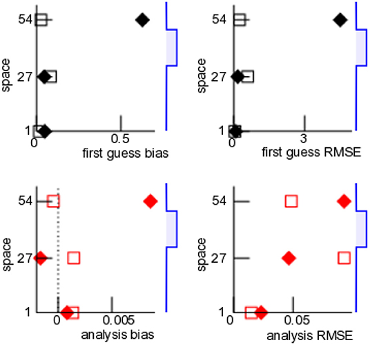
Figure 1. Example for effect of nonlocal observations on departure statistics. Verification of model equivalents in observation space by local observations at three spatial positions (x = 1, 27, and 54) for assimilation of local observations only (open squares) and assimilation of local observations and nonlocal observation (solid diamonds). The blue-colored line sketch on the right hand side reflects the sensitivity function of the nonlocal observation with center at x = 40 and the width r_H = 10; the localization radius is r_l = 10. Further details on the model, observations and assimilation parameters are given in section 2.7.

Section 2 introduces the essential elements of the LETKF and re-calls its analytical description for a single observation in section 2.5. Section 2.8 provides conventional and new markers of filter divergence that help to elucidate possible underlying divergence mechanisms. Section 3 presents briefly the findings, that are put into context in section 4.

2. Methods

2.1. The Model

The storm-like Lorenz96—model [23] is a well-established meteorological model and the present work considers an extension by a space-dependent linear damping [24]. It is a circle network with nodes of number N, whose node activity x_k(t) at node k and time t obeys

$\begin{array}{l}\frac{d{x}_k}{dt}=(x_{k+1}-x_{k-2})x_{k-1}\\ \begin{array}{l}-(1/2+2{\text{ cos}}^4({\alpha }_k\pi ))x_k+I,\end{array}& (1)\end{array}$

with k = 1, …, N, x_k = x_k+N, and α_k = k/N. We choose I = 8.0 and N = 80 and the initial condition is random with x_k(0) = 8.0 + ξ_k, k ≠ N/2, and x_N/2(0) = 8.01 + ξ_N/2 with the normal distributed random variable $\xi ~{N}(0,0.01)$. Figure 2A shows the model field dependent on time.

FIGURE 2

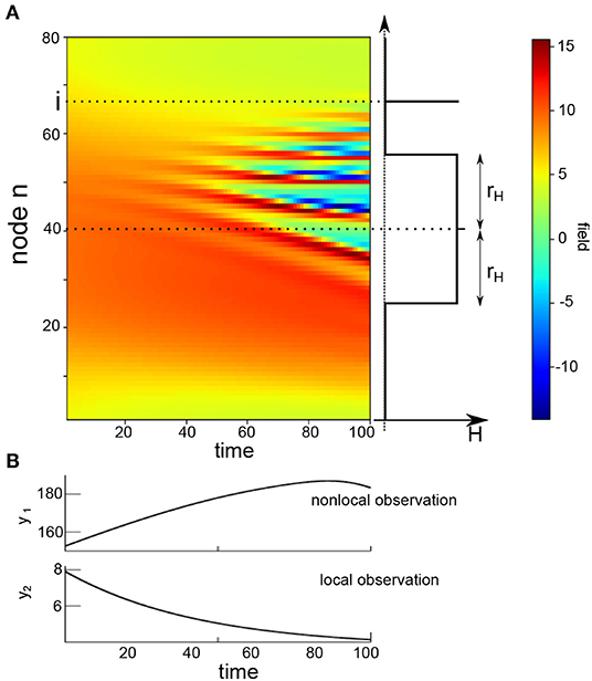
Figure 2. The model field V from Equation (1) and an illustration of the observation operator H from Equation (12) with the sensitivity function width r_H. (A) Exemplary space-time distribution of the model solution (left hand side) with the parameters I = 8.0 and N = 80, the sketched position i of a local observation and a sketched sensitivity function of nonlocal observation with the center in the middle of the spatial field with radius r_H. (B) Example observations illustrating that local and nonlocal observations are scalars and may evolve differently over time. Please also note the different order of values of the two observation types.

Typically, data assimilation techniques are applied to merge observations and solutions of imperfect models and the true dynamics of the underlying system is not known. To illustrate the impact of nonlocal observations, we assume (what is unrealistic in practice) that the model under consideration (1) is perfect and hence emerging differences between observations and model equivalents do not originate in the model error.

2.2. The Local Ensemble Transform Kalman Filter (LETKF)

The aim of data assimilation is to estimate a state that describes optimally both a model (or background) state x^b ∈ ℝ^N and corresponding observations y ∈ ℝ^S of number S. This analysis x^a ∈ ℝ^N minimizes the cost function

$\begin{array}{l}J(x)={\left(x-x^b\right)}^t{B}^{-1}\left(x-x^b\right)+\\ +{\left(y-\widehat{H}(x^b)\right)}^t{R}^{-1}\left(y-\widehat{H}(x^b)\right)& (2)\end{array}$

with x ∈ ℝ^N, the background error covariance B ∈ ℝ^N×N and the observation error covariance R ∈ ℝ^S×S. The observation operator $\widehat{H}$:ℝ^N → ℝ^S is linear in the present work and projects a model state into the observation space and thus links model and model equivalents in observation space.

The LETKF estimates the background error covariance B by background-ensemble perturbations of number L

$\begin{array}{ll}B\approx \frac{1}{L-1}{X}^b{\left(X^b\right)}^t& (3)\end{array}$

with X^b ∈ ℝ^N×L. In the following, we will call an ensemble with L = N a full ensemble, compared to a reduced ensemble with the typical case L < N. The columns of X^b are the background ensemble member perturbations $\left\{x^{b,l}-{\overline{x}}^b\right\}\forall l=1,\dots ,L$, {x^b,l} is the set of background ensemble members and ${\overline{x}}^b$ is the mean over the ensemble.

Then the coordinate transformation from physical space to ensemble space

$\begin{array}{ll}x={\overline{x}}^b+X^{b}w& (4)\end{array}$

describes a state x in the ensemble space with new coordinates w [7]. Inserting Equation (4) into (2) yields

$\begin{array}{l}J(w)=(L-1)w{w}^t\\ +{\left(y-{\overline{y}}^b-Yw\right)}^t{R}^{-1}\left(y-{\overline{y}}^b-Yw\right)& (5)\end{array}$

in the new coordinate w. Here ${\overline{y}}^b=\widehat{H}({\overline{x}}^b)\in {ℝ}^S$ is the model equivalent of the background ensemble mean in observation space and Y^b = $\widehat{H}$(X^b) is the corresponding model equivalent of X^b. This implies [7]

$\begin{array}{l}\widehat{H}\left(\overline{x}+X^{b}w\right)\approx {\overline{y}}^b+Y^{b}w,\end{array}$

which is valid for linear observation operators.

The minimization of the cost function (5) yields

$\begin{array}{ll}{\overline{w}}^a=A{(Y^b)}^t{R}^{-1}\left(y-{\overline{y}}^b\right)& (6)\end{array}$

with

$\begin{array}{ll}A={\left[(L-1)I+{\left(Y^b\right)}^t{R}^{-1}{Y}^b\right]}^{-1}.& (7)\end{array}$

Equation (4) provides the analysis ensemble mean

$\begin{array}{ll}{\overline{x}}^a={\overline{x}}^b+X^b{\overline{w}}^a.& (8)\end{array}$

Then the square root filter-ansatz [7] yields the analysis ensemble members

$\begin{array}{l}{w}^{a,l}={\overline{w}}^a+W^{a,l},\end{array}$

where W^{a, l} is the l-th column of the matrix W^a = [(L − 1)A]^1/2. The square root of A may be computed by using the singular value decomposition A = UDV^t with the diagonal matrix D and the eigenvector matrices U, V. This yields A^1/2 = UD^1/2V^t.

Finally the analysis ensemble members in physical space read

$\begin{array}{ll}{x}^{a,l}={\overline{x}}^b+X{\overline{w}}^a+X{W}^{a,l},l=1,\dots ,L,& (9)\end{array}$

see [7, 8] for more details.

Specifically, we have chosen L = 10 ensemble members and number of observations S = 1 or S = 2.

2.3. Observation Data

In principle there are two types of observations. Local observations are measured at a single spatial location in the system, whereas nonlocal observations are integrals over a set of spatial locations. Examples for local observations are radiosondes measuring humidity and temperature in the atmosphere at a certain vertical altitude and horizontal position. Typical nonlocal observations are satellite measurements capturing the radiation in a vertical atmospheric column.

The present work considers observations

$\begin{array}{ll}y=\widehat{H}(x)+\eta ,& (10)\end{array}$

where η ∈ 𝕊 is Gaussian white noise with the true variance R_t and $\widehat{H}$(x) is a linear observation operator $\widehat{H}$(x) = Hx, H ∈ ℝ^S×N. In the following, the linear operator H is called sensitivity function and we adopt this name from meteorological data assimilation of nonlocal satellite data. The present work considers either nonlocal observations only (S = 1) with the observation matrix elements

$\begin{array}{ll}{H}_{1n}=\{\begin{array}{cc}1\hfill & n\in [N/2-r_H;N/2)\hfill \\ 1+10^{-5}\hfill & n=N/2\hfill \\ 1\hfill & n\in (N/2;N/2+r_H]\hfill \\ 0\hfill & \text{otherwise}\hfill \end{array}\hfill & (11)\end{array}$

with sensitivity function width r_H or both observation types (S = 2), for which the observation matrix elements read

$\begin{array}{ll}{H}_{1n}=\{\begin{array}{cc}1\hfill & n\in [N/2-r_H;N/2)\hfill \\ 1+10^{-5}\hfill & n=N/2\hfill \\ 1\hfill & n\in (N/2;N/2+r_H]\hfill \end{array}\hfill & (12)\end{array}$

$\begin{array}{ll}{H}_{2n}=1\text{ for }n=i& (13)\end{array}$

$\begin{array}{ll}{H}_{km}=0\text{ otherwise},& (14)\end{array}$

where the local observation is captured at spatial location i, cf. Figure 2 for illustration. The sensitivity function of the nonlocal observation has a small peak in its center, which permits to localize the observation in the center of the sensitivity function, cf. section 2.4.

In the subsequent sections, i = N/2 and r_H varies in the range 1 ≤ r_H ≤ 10. Please note that r_H = 1 approximates the model description of a local observation. Moreover, in the following a grid point whose activity contributes to a model equivalent in observation space is called an observed grid point and all others are called unobserved grid points. Mathematically, observed (unobserved) grid points exhibit H_nk ≠ 0 (H_nk = 0).

In this work, a single partial study considers a smooth sensitivity function instead of the boxcar function described above. Then the sensitivity function is the Gaspari-Cohn function GC(n, r_H/2) [25] in the interval −r_H ≤ n ≤ r_H, which approximates the Gaussian function by a smooth function with finite support 2r_H

$\begin{array}{l}{H}_{1n}=\{\begin{array}{cc}GC(n,r_H)\hfill & n\in \left[-r_H;r_H\right]\hfill \\ 0\hfill & \text{otherwise}\hfill \end{array}\hfill \end{array}$

The observations y(t_n), t_n = 1, …, T at T time instances (cf. Equation 10) obey the model (1) and Equation (10) with the observation operator (11) or (12). In a large part of the work, we have assumed zero observation error R_t = 0, i.e., observations are perfect in the sense that they reflect the underlying perfect model, cf. section 2.1. We take the point of view that we do not know that the model and observations are perfect and hence we guess R as it is done in cases where models and observations are not perfect.

This approach has been taken in most cases in the work. Since, however, this implicit filter error may already contribute to a filter instability or even may induce it, a short partial study has assumed perfect knowledge of the observation error. To this end, in this short partial study we have assumed (R_t)_jj = 0.1, j = 1, …, S and perfect knowledge of this error, i.e., R = R_t.

Although techniques have been developed to estimate R adaptively [26], we do not employ such a scheme for simplicity.

2.4. Localization

In the LETKF, the background covariance matrix B is expressed by L ensemble members, cf. Equation (3), and it is rank-deficit for L ≪ N. This leads to spurious correlations in B. Spatial localization in ensemble Kalman filters has been found to be beneficial [16, 27–29] in this context. The LETKF as defined by Hunt et al. [7] performs the localization in observation space. In detail, Hunt et al. [7] proposed to localize by increasing the observation error in matrix R dependent on the distance between the analysis grid point and observations. The present implementation follows this approach.

The observation error matrix R is diagonal, i.e., observation errors between single observations are uncorrelated. Then at each grid point i the localization scheme considers observations y_n at location j only if the distance between location i and j does not exceed the localization radius r_l. Then the error of observation n is $R_{nn}=R_{nn}^0/{\rho }_{ij}$, where ρ_ij = GC(d_ij, r) + ε for d_ij ≤ r_l is the weighting function with the Gaspari-Cohn function GC(d, r) [25], ε > 0 is a small constant ensuring a finite observation error and d_ij is the spatial distance between i and j. The Gaspari-Cohn function approximates a Gaussian function with standard deviation $r\sqrt{3/10}$ by a polynomial with finite support. The parameter 2r = r_l is the radius of the localization function with 0 ≤ GC(z, r) ≤ 1, 0 ≤ z ≤ r_l. Consequently the observation error takes its minimum $R_{nn}^0$ at distance d_ij = 0 and increases monotonously with distance to its maximum $R_{nn}^0/\epsilon$ at d_ij = r_l. In the present implementation, we use ε = 10⁻⁷ and observation errors $R_{11}^0=0.1$ for a single nonlocal observation S = 1 and $R_{nm}^0=0.1{\delta }_{nm},n=1,2$ for local and nonlocal observation with S = 2.

The observation error close to the border of the localization area about a grid point i is large by definition $R_{nn}=R_{nn}^0/(GC(d\to r_l/2,r_l/2)+\epsilon )$. In numerical practice, the assimilation effect of large values $R_{nn}>R_{nn}^0/G{C}_{\text{low}}$ is equivalent for some distances from the grid point i in a reasonable approximation if GC_low is low enough. By virtue of the monotonic decrease of GC(d, r_l/2) with respect to distance d ≥ 0, this yields the condition GC(r_l ≥ d ≥ r_c, r_l/2) < GC_low. In other words, for distances d larger than a corrected localization radius r_c, the observation errors R_nn are that large that observations at such distances do poorly contribute to the analysis. For instance, if GC_low = 0.01, then r_l = 5 → r_c = 3, r_l = 10 → r_c = 7 and r_l = 15 → r_c = 11. It is important to note that this corrected localization radius depends on the width of the Gaspari-Cohn function and thus on the original localization radius r_l, i.e., r_c = r_c(r_l). In most following study cases results are given for original localization radii r_l, while the usage of the corrected localization radius is stated explicitly. The existence of a corrected localization radius r_c illustrates the insight, that there is not a single optimal localization radius for smooth localization functions but a certain range of equivalent localization radii. For non-smooth localization functions with sharp edges, e.g., a boxcar function, this variability would not exist.

The present work considers primarily nonlocal observations. Since these are not located at a single spatial site, it is non-trivial to include them in the LETKF that assumes a single observation location. To this end, several previous studies have suggested corresponding approaches [13, 24, 30–36]. A reasonable approximation for the spatial location of a nonlocal observation is the location of the maximum sensitivity [10, 37], i.e., ${\text{max}}_n{H}_{kn}$ of nonlocal observation k. Although this approximation has been shown to yield good results, it introduces a considerable error for broad sensitivity functions, i.e., r_H is large. In fact, this localization scheme introduces an additional contribution to the observation error. The present implementation considers this definition. This results in the localization of the nonlocal observation at grid point i = N/2.

2.5. LETKF for a Single Observation

In a large part of this work, we consider a single observation with S = 1. The subsequent paragraphs show an analytical derivation of the ensemble analysis mean and the analysis members, whose terms are interpreted in section 3.

Considering the localization scheme described above, at the model grid point i the analysis ensemble mean (8) reads

$\begin{array}{ll}{\overline{x}}_i^a={\overline{x}}_i^b+\left(X_i{A}_i{Y}^t\right)(y_0-{\overline{y}}^b)/R_i& (15)\end{array}$

where Y ∈ ℝ^L is a row vector with $Y_k=Y_{1k}^b$, with the row vector $X_i\in {ℝ}^L,{(X_i)}_k=X_{ik}$ and

$\begin{array}{ll}{A}_i={\left[(L-1)I+Y^{t}Y/R_i\right]}^{-1}.& (16)\end{array}$

The term $R_i=R_{11}^0/{\rho }_{i(N/2)}$ denotes the weighted observation error used at grid point i, when the observation is located at j = N/2, and $R_{11}^0$ is the error of observation y₁.

Now utilizing the Woodbury matrix identity [38]

$\begin{array}{l}{(B+UCV)}^{-1}=\\ B^{-1}-B^{-1}U{(C^{-1}+V{B}^{-1}U)}^{-1}{\text{V}\text{B}}^{-1}\end{array}$

for real matrices B ∈ ℝ^n×n, U ∈ ℝ^n×k, C ∈ ℝ^k×k, and V ∈ ℝ^k×n with n, k ∈ ℕ, Equation (16) reads

$\begin{array}{l}{A}_i=\frac{1}{L-1}{Q}_i\\ \begin{array}{l}{Q}_i=I-\frac{1}{(L-1)R_i+y^2}{Y}^{t}Y,\end{array}& (17)\end{array}$

where $y=\sqrt{{YY}^t}\in ℝ$ is a scalar. Inserting (17) into (15), the analysis ensemble mean is

$\begin{array}{ll}{\overline{x}}_i^a={\overline{x}}_i^b+X_i{Y}^t{\alpha }_i& (18)\end{array}$

with

$\begin{array}{l}{\alpha }_i=\frac{y_0-{\overline{y}}^b}{(L-1)R_i+y^2}.\end{array}$

Since $R_{N/2}=R_{11}^0$ and $R_{N/2\pm r_l}=R_{nn}^0/\epsilon =10^7{R}_{nn}^0$, α_i takes its maximum at the observation location and is very small when the observation is at the localization border. This means that ${\overline{x}}_i^a\approx {\overline{x}}_i^b$ at the border of the localization area.

Now let us focus on the ensemble members. Equations (18) and (9) give the analysis ensemble members at grid point i

$\begin{array}{ll}{x}_i^{a,l}={\overline{x}}_i^b+X_i{Y}^t{\alpha }_i+\sqrt{L-1}{X}_i{\left(\sqrt{A_i}\right)}_l,& (19)\end{array}$

where ${(\sqrt{A_i})}_l$ is the l-th column of matrix $\sqrt{A_i}=\sqrt{Q_i}/\sqrt{L-1}$.

The singular value decomposition serves as a tool to compute

$\begin{array}{ll}\sqrt{Q_i}=U\sqrt{D}{U}^t,& (20)\end{array}$

where $\sqrt{D}\in {ℝ}^{L\times L}$ is diagonal and its matrix elements are the eigenvalues of Q. The columns of matrix U ∈ ℝ^L×L are the normalized eigenvectors of Q. Then Equation (7) yields

$\begin{array}{l}{Q}_i{Y}^t=\left(I-\frac{1}{(L-1)R_i+y^2}{Y}^{t}Y\right)Y^t\\ =Y^t-\frac{y^2}{(L-1)R_i+y^2}{Y}^t\\ =\frac{(L-1)R_i}{(L-1)R_i+y^2}{Y}^t\\ ={\lambda }_i{Y}^t,\end{array}$

i.e., Y^t is an eigenvector of Q_i with eigenvalue 0 < λ_i < 1. By virtue of the properties of R_i, λ_i takes its minimum at the observation location at i = N/2 and it is maximum at the localization border.

The remaining eigenvectors of number L − 1 are v_n ⊥ Y, n = 1, …, L − 1 with unity eigenvalue since

$\begin{array}{l}{Q}_i{v}_n=\left(I-\frac{1}{(L-1)R_i+y^2}{Y}^{t}Y\right)v_n\\ =v_n-\frac{1}{(L-1)R_i+y^2}{Y}^t{\displaystyle \underset{=0}{{\displaystyle \underbrace{Y{v}_n}}}}\\ =v_n.\end{array}$

Hence $U=(Y^t/\Vert Y\Vert ,v_1,\dots ,v_{L-1})$ and $\sqrt{D}=\text{diag}(\sqrt{{\lambda }_i},1,\dots )$ and, after inserting into Equation (20) and lengthy calculations

$\begin{array}{ll}{(\sqrt{Q_i})}_{kl}=\sqrt{{\lambda }_i}\frac{Y_k{Y}_l}{y^2}+{\displaystyle \sum _{n=1}^{L-1}}{(v_n)}_k{(v_n)}_l.& (21)\end{array}$

This leads to

$\begin{array}{ll}{x}_i^{a,l}={\overline{x}}_i^b+X_i{Y}^t{\alpha }_i+X_i{Y}^t\frac{\sqrt{{\lambda }_i}}{y^2}{Y}_l+{\displaystyle \sum _{n=1}^{L-1}}{X}_i{v}_n{(v_n)}_l.& (22)\end{array}$

2.6. Additive Covariance Inflation

The ensemble Kalman filter underestimates the forecast error covariance matrix due to the limited ensemble size [39]. This problem is often addressed by covariance inflation [27, 40, 41]. The present work implements additive covariance inflation [42]. The ensemble perturbations X^b in (3) are modified by white Gaussian additive noise Γ ∈ ℝ^N×L

$\begin{array}{l}{X}_{\text{add}}^b=X^b+\Gamma .\end{array}$

with matrix elements ${\Gamma }_{ij}~{N}(0,f_{add}^2)$ and the inflation factor f_add = 0.1.

2.7. Numerical Experiments

The present study investigates solutions x(t) of model (1) and Equation (10) provides the observations y(t). This is called the nature run. In the filter cycle, the initial analysis values are identical to the initial values of the nature run and the underlying filter model is the true model (1). In the forecast step, the model is advanced with time step Δt = 10⁻³/12 for 100 time steps applying a 4th-order Runge-Kutta integration scheme. According to [23], the duration of one forecast step corresponds to 1 hour which is also the time between two successive observations. The analysis update is instantaneous. In an initial phase, the model evolves freely for 50 forecast steps, i.e., 50 h, to avoid possible initial transients. Then, the LETKF estimates the analysis ensemble according to section 2.2 during 200 cycles if not stated otherwise. One of such a numerical simulation is called a trial in the following and it comprises 100·200 time steps. In all figures, the time given is the number of forecast steps, or equivalently analysis steps in hours.

Each trial assumes identical initial ensemble members and the only difference in trials results from the additive noise in additive covariance inflation, cf. section 2.6.

By virtue of the primarily numerical nature of the present work, it is mandatory to vary certain parameters, such as perturbations to the observations or the factor of additive inflation. For instance, the data assimilation results in Figure 1 are based on model (1), 3 local and 1 nonlocal observation. This corresponds to the observation operator $\widehat{H}$ with the sensitivity function

$\begin{array}{l}{H}_{1n}={\delta }_{n{n}_1}\\ H_{2n}={\delta }_{n{n}_2}\\ H_{3n}={\delta }_{n{n}_3}\\ H_{4n}=\{\begin{array}{cc}1\hfill & n\in [N/2-r_H;N/2)\hfill \\ 1+10^{-5}\hfill & n=N/2\hfill \\ 1\hfill & n\in (N/2;N/2+r_H]\hfill \end{array}\hfill \end{array}$

with r_H = 10 and n₁ = 1, n₂ = 27, n₃ = 54. The localization radius is identical to the sensitivity function r_l = r_H and data assimilation is performed during 250 filter cycles with an initial phase of 50 forecast steps. For stabilization reasons, we have increased the model integration time step to Δt = 10⁻²/12 but reduced the number of model integrations to 10 steps, cf. [19], thus essentially retaining the time interval between observations. Other parameters are identical to the standard setting described in the previous sections.

As mentioned above, typically the measurement process is not known in all details. For instance, the observation error is assumed to be R = 0.1 for the nonlocal observations, whereas the true model exhibits noise-free observations with R_t = 0. This is the valid setting for all simulations but few set of trials shown in Figure 5. In a set of experiments [Figure 5 (solid, dashed, and dashed-dotted line)], observations are noisy with noise perturbation variance 0.1 and hence R_t = R = 0.1. Moreover, the additive inflation factor is chosen to f_add = 0.1 but in two single sets of experiments [cf. Figure 5 (dashed and dashed-dotted line)], where f_add = 0.05. In addition, the weighting function of nonlocal observations is a boxcar window function with sharp borders but in a single set of experiments, where the weighting function is a smooth Gaspari-Cohn function, cf. Figure 5 (dashed-dotted line).

The verification measures bias and RMSE are computed for the local observations only according to Equations (23) and (24).

2.8. Divergence Criteria and Verification

The Kalman filter may diverge for several reasons [6, 27, 43], such as model error, insufficient sampling of error covariance, or high condition number of observation operators [17, 44]. Especially the latter has been shown to be able to trigger catastrophic filter divergence of the ensemble Kalman filter exhibiting a diverging forecasts in model state space [19–21]. This divergence type exhibits a magnitude increase of model variables to machine infinity in finite time. The present implementation detects catastrophic filter divergence and stop the numerical simulation when the maximum absolute value of any single ensemble member exceeds a certain threshold $|x_k^{b,l}|>10^{10},k\in \left[1;N\right],l\in \left[1;L\right]$.

The present work focusses primarily on a non-catastrophic filter divergence type showing a strong increase of the innovation magnitude to values much larger than the model equivalent in observation space of the attractor. This divergence may be temporally intermittent with finite duration. Since this intermittent innovation divergence results in increased first guess departures and hence worsens forecasts, it is important to detect these divergences and control them. By definition the innovation process diverges if ${\text{max}}_{l,k}\left|{[y_n-{Hx}^{b,l}]}_k\right|>{\sigma }_{th}$ for any observation n with ${\sigma }_{th}=1,000\sqrt{R_{nn}^0}$. Then the numerical simulation is stopped. The time of filter divergence is called T_b in the following. This criterion for innovation divergence is hard: if the innovation reaches the threshold σ_th, then innovation divergence occurs. The corresponding divergence rate γ is the ratio between the number of divergent and non-divergent trials. For instance, for γ = 1 all numerical trials diverge whereas γ = 0 reflect stability in all numerical trials.

Moreover, it is possible that $\left|{[y_n-{Hx}^{b,l}]}_k\right|$ grows intermittently but does not reach the divergence threshold. The first guess departure bias

$\begin{array}{ll}\text{bias}=\frac{1}{TS}{\displaystyle \sum _{k=1}^T}{\displaystyle \sum _{n=1}^S}{[y(t_k)]}_n-{[H{\overline{\text{x}}}^b(t_k)]}_n& (23)\end{array}$

and the corresponding root mean-square error

$\begin{array}{ll}\text{RMSE}=\frac{1}{TS}{\displaystyle \sum _{k=1}^T}{\displaystyle \sum _{n=1}^S}{(y_n(t_k)-{[H{\overline{\text{x}}}^b(t_k)]}_n)}^2& (24)\end{array}$

quantify the forecast error in such trials. For a single observation, y → y_o. Larger values of bias RMSE indicate larger innovation values.

To quantify filter divergence, Tong et al. [18] have proposed the statistical measure

$\begin{array}{l}{\Theta }_n=\sqrt{\frac{1}{L}{\displaystyle \sum _{l=1}^L}{(y(t_n)-{Hx}^{b,l}(t_n))}^t(y(t_n)-{Hx}^{b,l}(t_n))}\end{array}$

and

$\begin{array}{l}{\Xi }_n=\Vert \frac{1}{L-1}{\displaystyle \sum _{l=1}^L}{\text{X}}_o(t_n)\otimes {\text{X}}_u(t_n)\Vert \end{array}$

at time t_n, where the norm is defined by $\Vert \text{Z}\Vert =\sum _{n,m}|Z_{nm}{|}^2$ for any matrix Z and Z_nm are the corresponding matrix elements. The quantity Θ_n represents the ensemble spread in observation space and Ξ_n is the covariation of observed and unobserved ensemble perturbations assuming local observations. Large values of Ξ indicates catastrophic filter divergence as pointed out in [18, 20]. This definition may also apply to nonlocal observations, cf. section 2.5, although its original motivation assumes local observations.

An interesting feature to estimate the degree of divergence is the time of maximum ensemble spread T_Θ and the time of maximum covariation of observed and unobserved ensemble perturbations T_Ξ:

$\begin{array}{l}{T}_{\Theta }=\text{arg }{\displaystyle \underset{n}{\text{max}}}{\Theta }_n\\ T_{\Xi }=\text{arg }{\displaystyle \underset{n}{\text{max}}}{\Xi }_n.& (25)\end{array}$

Moreover, previous studies have pointed out that catastrophic filter divergence in ensemble Kalman filter implies alignment of ensemble members. This may also represent an important mechanism in non-catastrophic filter divergence. The new quantity

$\begin{array}{ll}{p}_{a,u}=\frac{n_{a,u}}{L(L-1)/2}& (26)\end{array}$

is the probability of alignment and unalignment, where n_a is the number of aligned ensemble member perturbation pairs $({\text{x}}^{b,l}-{\overline{\text{x}}}^b),({\text{x}}^{b,k}-{\overline{\text{x}}}^b)$ for which

$\begin{array}{l}\text{cos }{\beta }_{lk}=\frac{{({\text{x}}^{b,l}-{\overline{\text{x}}}^b)}^t({\text{x}}^{b,k}-{\overline{\text{x}}}^b)}{\Vert {\text{x}}^{b,l}-{\overline{\text{x}}}^b\Vert \Vert {\text{x}}^{b,k}-{\overline{\text{x}}}^b\Vert }\ge 0.5\end{array}$

and n_u is the number of ant-aligned member pairs with

$\begin{array}{l}\text{cos }{\beta }_{lk}=\frac{{({\text{x}}^{b,l}-{\overline{\text{x}}}^b)}^t({\text{x}}^{b,k}-{\overline{\text{x}}}^b)}{\Vert {\text{x}}^{b,l}-{\overline{\text{x}}}^b\Vert \Vert {\text{x}}^{b,k}-{\overline{\text{x}}}^b\Vert }\le -0.5\end{array}$

∀l ≠ k, l, k = 1, …, L. The alignment (anti-alignment) condition cos β_lk > 0.5 (cos β_lk < −0.5) implies $-60^{.}\le {\beta }_{lk}\le 60^{.}$ ($120^{.}\le {\beta }_{lk}|\le 240^{.}$). Please note that 0 ≤ p_a,u ≤ 1 and the larger p_a (p_u) the more ensemble members are aligned (anti-aligned) to each other.

Considering the importance of member alignment to each other for catastrophic divergence, it may be interesting to estimate the alignment degree of background member perturbation with the analysis increments x^{a, l} − x^b,l by

$\begin{array}{ll}\text{cos }{\alpha }_l=\frac{{({\text{x}}^{b,l}-{\overline{\text{x}}}^b)}^t({\text{x}}^{a,l}-{\text{x}}^{b,l})}{\Vert {\text{x}}^{b,l}-{\overline{\text{x}}}^b\Vert \Vert {\text{x}}^{a,l}-{\text{x}}^{b,l}\Vert },l=1,\dots ,L.& (27)\end{array}$

The term x^{a, l} − x^b,l is the analysis ensemble member perturbation from the background members and ${\text{x}}^{b,l}-{\overline{\text{x}}}^b$ is the direction of the background member perturbation. If cos α_l → 1 (cos α_l → −1) the analysis ensemble members point into the same (opposite) direction as the background ensemble members. In addition,

$\begin{array}{ll}{q}_a=\frac{n_a}{L},q_u=\frac{n_u}{L}& (28)\end{array}$

are the percentages of aligned and anti-aligned ensemble members for which cos α_l > 0.5 (of number n_a) and cos α_l < −0.5 (of number n_u), respectively.

3. Results

The stability of the ensemble Kalman filter depends heavily on the model and the nature of observations. To gain some insight into the effect of nonlocal observations, the present work considers primarily nonlocal observations only (section 3.1). Then the last section 3.2 shows briefly the divergence rates in the presence of both local and nonlocal observations.

3.1. Nonlocal Observations

The subsequent sections consider nonlocal observations only and show how they affect the filter stability. To this end, the first studies are purely numerical and are complemented by an additional analytical study.

3.1.1. Numerical Results

In order to find out how the choice of localization radius r_l affects the stability of the LETKF, a large number of numerical experiments assist to investigate statistically under which condition the filter diverges. Figure 3 shows the temporal evolution of the background x^b and the model equivalents in observation space y^b for two different localization radii. In Figure 3A, observations (black line) are very close to their model equivalents (blue lines) for identical localization and sensitivity function width, i.e., r_l = r_H. Conversely, observations and their model equivalents diverge after some time for r_l ≠ r_H. This is visible in the ensemble mean (Figure 3A, top row) and the single ensemble members (Figure 3A, bottom row). The different filter behavior can be observed in model space as well, but there it is less obvious, cf. Figure 3B. The ensemble members at spatial location n = 40 are located in the center of the observation area. They exhibit a rather small spread around the ensemble mean for r_l = r_H, whereas the ensemble spread is larger for r_l ≠ r_H. The ensemble at n = 20 is outside the observation area and thus is not updated. There, the ensemble in r_l = r_H and r_l ≠ r_H are close to each other.

FIGURE 3

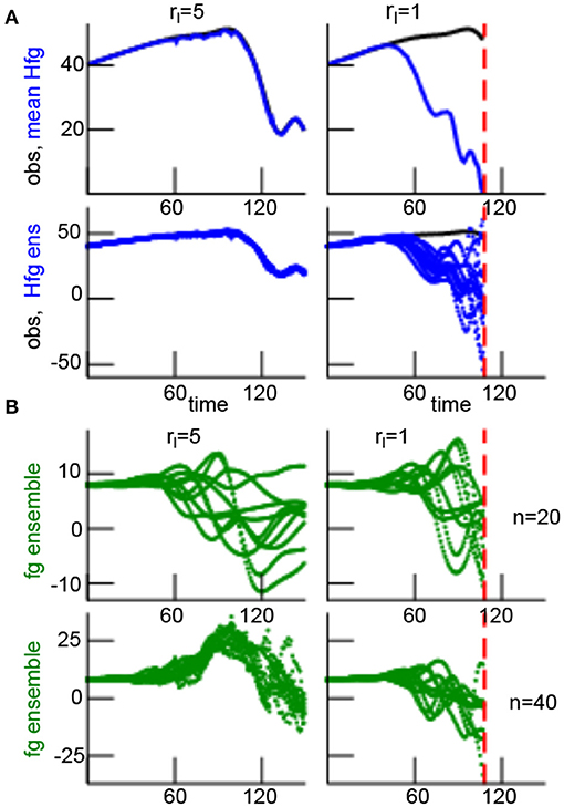
Figure 3. Temporal solutions of the filter process with r_H = 5 with two different localization radii r_l. (A) Comparison of observations (black line) and model equivalents in the observation space of the ensemble mean y^b [top row, solid blue line, denoted as Hfg for model equivalent (H) of the first guess (fg)] and the ensemble members y^(b,l) (bottom row, dotted blue line). The time represents the number of analysis steps. (B) First guess (fg) ensemble members in model space at the single spatial location n = 20 (shown in top panel), i.e., outside the observation area with H_1n = 0, and at the single spatial location n = 40, i.e., in the center of the observation area (shown in bottom panel).

This result can be generalized to a larger number of localization and sensitivity function widths, cf. Figure 4. For the smallest sensitivity function width and thus the smallest observation area with r_H = 1, no filter process diverges for a large range of localization radii r_l, i.e., the LETKF is stable (dashed black line in Figure 4). This case r_H = 1 corresponds to local observations. Now increasing the observation area with r_H > 1, the filter may diverge and its divergence rate γ depends on the localization radius. We observe that the filter diverges least when the localization radius is close to the sensitivity function width. These findings hold true for both the original localization radius and the corrected radius r_c, cf. section 2.4 and Figures 4A,B. Moreover, the filter does not exhibit catastrophic divergence before the background reaches its divergence threshold.

FIGURE 4

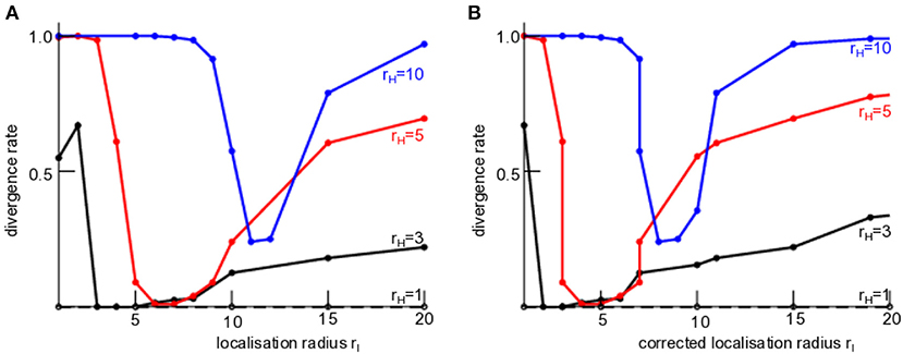
Figure 4. Stability of the LETKF of nonlocal observations dependent on the sensitivity function width r_H and the localization radius r_l. The divergence rate γ is defined in section 2.8. (A) With original localization radius r_l. (B) With corrected localization radius r_c and GC_low = 0.01. Here, the observations are noise-free with R_t = 0 but the chosen observation error is assumed to R = 0.1 ≠ R_t due to lack of knowledge of this true value.

These results hold also true if observations are subjected to additive noise and the observation error is chosen to the true value, cf. Figure 5 (solid line) and if additive inflation is chosen to a lower value [Figure 5 (dashed line)]. Similarly to Figure 4, the divergence rate is minimum if the sensitivity function width is close to the original (Figure 5A) or corrected (Figure 5B) localization radius r_l. The situation is different if the sensitivity function is not a non-smooth boxcar function as in the majority of the studies but a smooth Gaspari-Cohn function. Then the divergence rate is still minimum but the corresponding localization radius of this minimum is much smaller than r_H, cf. dotted-dashed line in Figure 5.

FIGURE 5

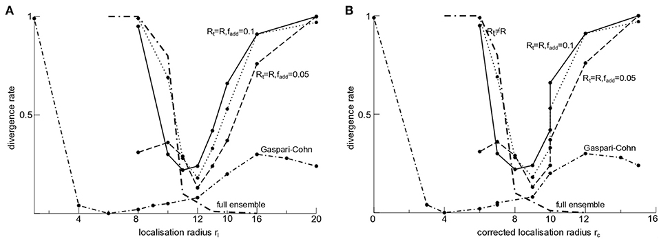
Figure 5. LETKF stability for different parameters and r_H = 10. The solid line denotes the divergence rate γ if the true observation error R_t = 0.1 is known, i.e., R = R_t, and the inflation rate is f_add = 0.1; the dashed line denotes the divergence rate for lower inflation rate f_add = 0.05, otherwise identical to the solid line case; the dotted-dashed line marks results identical to the dashed line case but with a smooth Gaspari-Cohn sensitivity function. The dotted line is taken from Figure 4 for comparison (R_t = 0, R = 0.1) and the bold dotted-dashed line represents the results with an ensemble L = 80, otherwise identical to the dotted line-case. (A) original localization radius r_l. (B) Corrected localization radius r_c with GC_low = 0.01.

All these results consider the realistic case of a small number of ensemble members L ≪ N. Nevertheless, it is interesting to raise the question how these results depend on the ensemble size. Figure 5 (bold dotted-dashed line) indicates that an ensemble with L = N = 80 may yield maximum divergence for r_l < r_H and stability with zero divergence rate for r_l > r_H. This means the full ensemble does not show a local minimum divergence rate as observed for L < N.

The divergence criterion is conservative with a hard threshold and trials with large but sub-threshold innovations, i.e., with innovations that do not exceed the threshold, are not detected as being divergent. Nevertheless to quantify intermittent large innovations in the filter, Figure 6 shows the bias and RMSE of trials whose innovation process do not reach the divergence threshold. We observe minimum bias and RMSE for original localization radii r_l that are similar to the sensitivity function width r_H (Figure 6A). For corrected localization radii r_c and r_H agree well at minimum bias and RMSE, cf. Figure 6B.

FIGURE 6

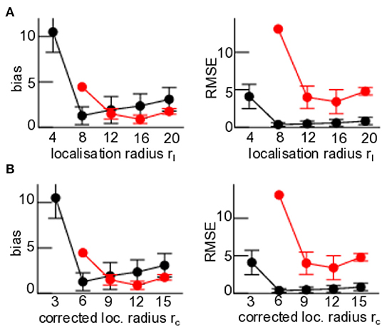
Figure 6. First guess departure statistics of trials that do not reach the divergence threshold. Here r_H = 5 (black) and r_H = 10 (red). (A) Original localization radius r_l. (B) Corrected localization radius r_c with GC_low = 0.01. All statistical measures are based on 100 trials.

Now understanding that localization radii r_l ≠ r_H may destabilize the filter, the question arises where this comes from and which mechanisms may be responsible for the innovation divergence. Figure 7 illustrates various statistical quantities for three exemplary trials. These quantities have been proposed to reflect or explain divergence. The innovation-based measure Θ_n diverges (Figure 7B) when the filter diverges (Figure 7A) for r_l < r_H and r_l ≫ r_H, whereas Θ_n remains finite for r_l ≈ r_H. Interestingly, for r_l < r_H a certain number of ensemble members align and anti-align intermittently but do not align in the instance of divergence (Figure 7C). In the case of similar localization radius and sensitivity function width, a similar number of ensemble members align and anti-align but the filter does not diverge. Conversely, for r_l ≫ r_H ensemble members both align and anti-align while the filter diverges. These results already indicate a different divergence mechanism for r_l ≤ r_H and r _> r_H. Accordingly, for r_l < r_H and r_l ≈ r_H background member perturbations align with the analysis member perturbations with cos α_l → 1 (Figure 7D), whereas cos α_l fluctuates between 1 and −1 for r_l ≫ r_H while diverging.

FIGURE 7

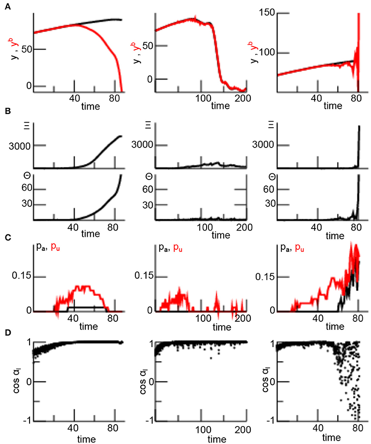
Figure 7. Various measures reflecting stability of the LETKF dependent on the localization radius r_l in single trials. (A) observation y_o (black) and its model equivalent $H{\overline{x}}^b$ (red). (B) Statistical quantities Ξ_n (top) and Θ_n (bottom), for definition see section 2.8. (C) The probability of ensemble member alignment according to Equation (26) for aligned (black) and anti-aligned (red) members. (D) Statistical estimate of alignment between ensemble members and x^a − x^b according to Equation (27). The different localization radii are r_l = 1 (left panel), r_l = 6 (center panel), and r_l = 20 (right panel) with the sensitivity function width r_H = 5.

Figure 8A shows the distribution of time instances T_Θ and T_Ξ when the respective quantities Θ_n and Ξ_n are maximum. These time instances agree well with the divergence times T_b. This confirms the single trial finding in Figures 7A,B that Θ_n and Ξ_n are good markers for filter innovation divergence. Moreover only few background members align and anti-align for r_l ≤ r_H (small values of p_a,u), whereas many more background members align and anti-align for r_l ≫ r_H (Figure 8B). Conversely, each analysis member aligns with its corresponding background member for r_l ≤ r_H (q_a = 1, q_u = 0) and most analysis members still align with their background members for r_l ≫ r_H (Figure 8C). This means that nonlocal observations do poorly affect the direction of ensemble members in these cases.

FIGURE 8

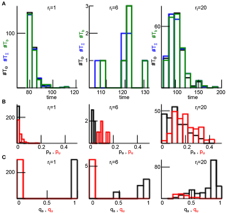
Figure 8. Divergence times and ensemble member alignment dependent on the localization radius r_l. (A) Histogram of time of maximum Θ_n (T_Θ, black), time of maximum Ξ_n (T_Ξ, blue), and the divergence time T_b (green), see the Methods section 2.8 for definitions. (B) Histograms of alignment ratio p_a (black) and anti-alignment ratio p_u (red) defined in Equation (26). (C) Histograms of alignment ratio q_a (black) and anti-alignment ratio q_u (red) defined in Equation (28). In addition r_H = 5 and results are based on the 200 numerical trials from Figure 4.

3.1.2. Analytical Description

According to Figure 9, there are different possible configurations of the sensitivity function with respect to the localization area. The localization radius r_l may be smaller (cases 1) or larger (cases 2) than the sensitivity width r_H or both may be equal (cases 3). In addition, it is insightful to distinguish observed and unobserved grid points as already proposed in [18].

FIGURE 9

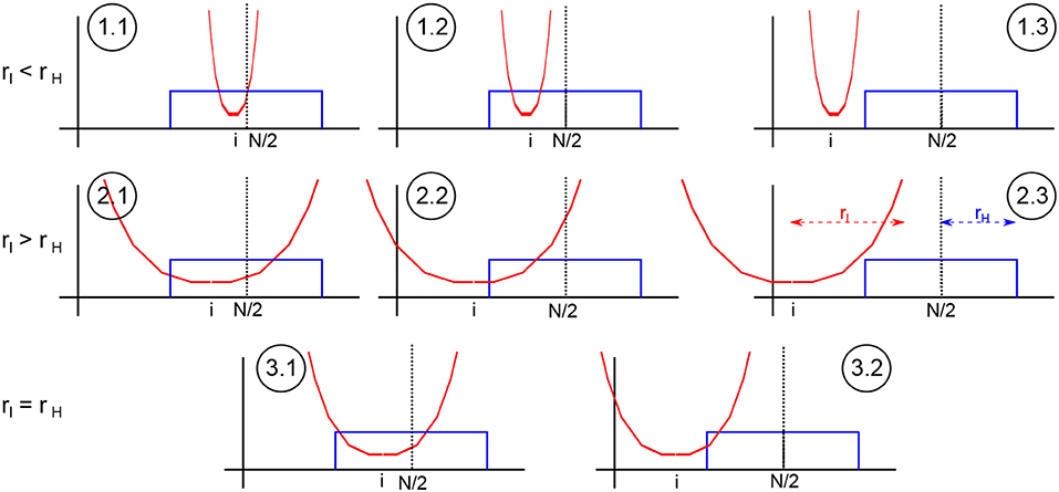
Figure 9. Sketch of different configurations of sensitivity function and localization area. The circles denote the different cases (n.m) The sensitivity function (blue) has its center at the center of the spatial domain and the localization function (red) is located about model grid element i.

Now let us take a closer look at each case, cf. Figure 9:

• $\underset{\_}{\text{case }1.1,r_l\le r_H,|i-\frac{N}{2}|\le r_H,\text{ and }|i-\frac{N}{2}|\le r_l}$: the localization radius is smaller than the sensitivity function width and the observation at spatial location N/2 is located within the localization radius about grid point i. Then, the analysis ensemble (22) and its mean (18) read

$\begin{array}{l}{x}_{o,i}^{a,l}={\overline{x}}_{o,i}^b+X_{o,i}{Y}^t{\alpha }_i+X_{o,i}{Y}^t\frac{\sqrt{{\lambda }_i}}{y^2}{Y}_l\\ \begin{array}{l}+{\displaystyle \sum _{n=1}^{L-1}}{X}_{o,i}{v}_n{(v_n)}_l\end{array}& (29)\end{array}$

and

$\begin{array}{ll}{\overline{x}}_{o,i}^a={\overline{x}}_{o,i}^b+X_{o,i}{Y}^t{\alpha }_i& (30)\end{array}$

with the corresponding ensemble means at observed grid points ${\overline{x}}_{o,i}^b$ and ${\overline{x}}_{o,i}^a$, the first guess perturbations X_o,i and the analysis ensemble members $x_{o,i}^{a,l}$.

• $\underset{\_}{\text{case }1.2,r_l\le r_H,|i-\frac{N}{2}|\le r_H,\text{ and }|i-\frac{N}{2}|>r_l}$: compared to case 1.1, the grid point i is observed as well but the observation is outside the localization area; hence the analysis is identical to the first guess

$\begin{array}{l}{\overline{x}}_{o,i}^a={\overline{x}}_{o,i}^b\\ x_{o,i}^{a,l}={\overline{x}}_{o,i}^b+{(X)}_{o,i}.\end{array}$

• case 1.3, r_l ≤ r_H, |i − N/2| > r_H, and |i − N/2| > r_l: the grid point i is not observed and the observation is outside the localization area leading to

$\begin{array}{l}{\overline{x}}_{u,i}^a={\overline{x}}_{u,i}^b\\ x_{u,i}^{a,l}={\overline{x}}_{u,i}^b+{(X)}_{u,i}& (31)\end{array}$

with the corresponding unobserved ensemble means ${\overline{x}}_{u,i}^b$ and ${\overline{x}}_{u,i}^a$, the unobserved ensemble perturbations X_u,i and the analysis ensemble member $x_{u,i}^{a,l}$.

• $\underset{\_}{\text{case }2.1,r_l>r_H,|i-\frac{N}{2}|\le r_H,\text{ and }|i-\frac{N}{2}|\le r_l}$: the localization radius is larger than the sensitivity function width, the observation is located within the localization radius about the grid point i and all grid points are observed. This case is equivalent to case 1.1 and the expressions for the analysis ensemble and mean hold as well.

• $\underset{\_}{\text{case }2.2,r_l>r_H,|i-\frac{N}{2}|>r_H,\text{ and }|i-\frac{N}{2}|\le r_l}$: compared to case 2.1, the observation is located within the localization radius but grid points are unobserved. Then

$\begin{array}{ll}{\overline{x}}_{u,i}^a={\overline{x}}_{u,i}^b+X_{u,i}{Y}^t{\alpha }_i& (32)\end{array}$

and

$\begin{array}{l}{x}_{u,i}^{a,l}={\overline{x}}_{u,i}^b+X_{u,i}{Y}^t{\alpha }_i+X_{u,i}{Y}^t\frac{\sqrt{{\lambda }_i}}{y^2}{Y}_l\\ \begin{array}{l}+{\displaystyle \sum _{n=1}^{L-1}}{X}_{u,i}{v}_n{(v_n)}_l.\end{array}& (33)\end{array}$

• $\underset{\_}{\text{case }2.3,r_l>r_H,|i-\frac{N}{2}|>r_H,\text{ and }|i-\frac{N}{2}|>r_l}$: in this case, the grid points are unobserved and the observation is outside the localization area. Then the analysis is identical to the first guess and the case is equivalent to case 1.3.

• $\underset{\_}{\text{case }3.1,r_l=r_H,|i-\frac{N}{2}|\le r_H}$: the observation is located within the localization radius about the grid point i, the grid point is observed and the expressions in case 1.1 hold.

• $\underset{\_}{\text{case }3.2,r_l=r_H,|i-\frac{N}{2}|>r_H}$: the observation is not located within the localization radius of grid point i, then grid point is not observed and the expressions in case 1.3 hold.

Firstly, let us consider the limiting case of local observations with r_H = 1. Then case 1 does not exist. This means that case 1 emerges for nonlocal observations only and Figure 4 demonstrates that the filter does not diverge for 1 ≤ r_l ≤ 20. Moreover, the sensitivity function of the observation is non-zero at the observation location only and hence the localization of the observation to the position of the sensitivity maximum (cf. section 2.4) is trivial. In case 2, this implies that updates at grid points far from the observation location i ≠ N/2 consider the local observation with weighted observation error R_i. This situation changes in case of nonlocal observations with r_H > 1. Then case 1 exists and analysis updates in case 2 consider an errornous estimate of the nonlocal observation at the single spatial location N/2. The broader the sensitivity function and thus the larger r_H, the larger is the error induced by this localization approximation. Consequently, updates at grid points far from the observation location still consider the observation with weighted observation error R_i, however the observation includes a much larger error than R_i introducing an analysis update error.

From a mathematical perspective, in cases 1.1, 2.1, and 3.1 the LETKF updates observed grid points whereas in the cases 1.3, 2.3, and 3.2 no update is applied. These cases appear to be consistent since grid points that contribute to the observation are updated by the observation and grid points that do not contribute to the observation are not updated. Conversely, observed grid points in case 1.2 do not consider the observation and are not updated although they contribute to the first guess in observation space. This missing update contributes to the filter error and the filter divergence as stated in previous work [12]. Moreover, the unobserved grid points in case 2.2 do consider the observation and are updated by the Kalman filter. At a very first glance, this inconsistency may be detrimental similar to case 2.1. However, it may be arguable whether this inconsistency may contribute to the filter error. On the one hand, the background error covariance propagates information from observed to unobserved grid points in each cycle step. This may hold true for system phenomena with a large characteristic spatial scale, such as wind advection or long-range moisture transport in meteorology or, more generally, emerging long-range spatial synchronization events. However, on the other hand, if the background error covariance represents a bad estimate, e.g., due to sampling errors or short-range synchronization, the false (or inconsistent) update may enhance errornous propagated information and hence contributes to the filter divergence. This agrees with the vanishing divergence in case of a full ensemble [cf. Figure 5 (bold dotted-dashed line)]. Moreover, updates at unobserved grid points may be errornous due to model errors or the approximation error made by replacing a nonlocal observation by an artificial observation at a single location. The larger the localization radius, the more distant are grid points to the observation location and the less representative is the localized observation to distant grid points.

Hence these two latter cases may cause detrimental effects. Consequently, cases 1 and 2, i.e., r_l ≠ r_H, yields bad estimates of analysis updates that make the Kalman filter diverge. Conversely, case 3, i.e., r_l = r_H, involves consistent updates only and detrimental effects as described for the other cases are not present. These effects may explain enhanced filter divergence for r_l ≠ r_H and minimum filter divergence for r_l = r_H seen in Figure 3, and the minimum divergence rate at r_l ≈ r_H shown in Figure 4.

The important terms in case 2.2, i.e., Equations (32) and (33), are $X_{u,i}{Y}^t,{\alpha }_i,\sqrt{{\lambda }_i}{Y}_l/y^2$, and $\sum _n{X}_{u,i}{v}_n{(v_n)}_l$. Equivalently, the missing terms in case 1.2 are $X_{o,i}{Y}^t,{\alpha }_i,\sqrt{{\lambda }_i}{Y}_l/y^2$ and $\sum _n{X}_{o,i}{v}_n{(v_n)}_l$. For instance,

$\begin{array}{ll}{c}_{o,u}=X_{o,u}{Y}^t={\displaystyle \sum _{l=1}^L}(x_{o,u}^{b,l}-{\overline{x}}_{o,u}^b)(y^{b,l}-{\overline{y}}^b)& (34)\end{array}$

and α_i appear in both cases 2.1 and 2.2. The terms c_o,u represent the covariances between model and model equivalents perturbations over ensemble members and they may contribute differently to the intermittent divergence with increasing |r_l−r_H|. For a closer investigation of these terms, let us consider

$\begin{array}{ll}{(c_o)}_i{\alpha }_i=X_{o,i}{Y}^t{\alpha }_i& (35)\end{array}$

in case 2.1 and

$\begin{array}{ll}{(c_u)}_i{\alpha }_i=X_{u,i}{Y}^t{\alpha }_i.& (36)\end{array}$

in case 2.2. These terms represent the weighted ensemble covariances between model and model equivalents perturbations in observation space. To quantify their difference,

$\begin{array}{l}{A}_o={\displaystyle \underset{n}{\text{max}}}\frac{1}{M_o}{\displaystyle \sum _{i\in {{M}}_o}}{(c_o)}_i(t_n){\alpha }_i(t_n)\\ A_u={\displaystyle \underset{n}{\text{max}}}\frac{1}{M_u}{\displaystyle \sum _{i\in {{M}}_u}}{(c_u)}_i(t_n){\alpha }_i(t_n)\\ A=A_o-A_u\end{array}$

may be helpful. The term A_o (A_u) is the maximum over time of the mean of (c_o)_iα_i ((c_u)_iα_i). This mean is computed over the set of observed (unobserved) grid points ${{M}}_o$ (${{M}}_u$) with size M_o (M_u). Consequently, A quantifies the difference of observed and unobserved weighted model-observation ensemble covariances, while the unobserved covariances are down-weighted by α_i compared to the observed covariances. This down-weighting results from the fact that unobserved grid points are more distant from the observation which yields smaller values of α_i. By definitions (35) and (36), thus A < 0 reflects larger weighted model-observation covariances in unobserved than observed grid points.

The corresponding quantities

$\begin{array}{l}{T}_o=\text{arg }{\displaystyle \underset{n}{\text{max}}}\frac{1}{M_o}{\displaystyle \sum _{i\in {{M}}_o}}{(c_o)}_i(t_n){\alpha }_i(t_n)\\ \begin{array}{l}{T}_u=\text{arg }{\displaystyle \underset{n}{\text{max}}}\frac{1}{M_u}{\displaystyle \sum _{i\in {{M}}_u}}{(c_u)}_i(t_n){\alpha }_i(t_n)\end{array}& (37)\end{array}$

$\begin{array}{ll}\Delta T=T_o-T_u& (38)\end{array}$

define the time instances when these maxima are reached and ΔT is their difference. For instance, if ΔT > 0, then the weighted model-observation covariances at observed grid points reach their maximum before weighted model-observation covariances at unobserved grid points.

To illustrate the importance of A_o and its corresponding occurrence time T_o, Figure 10 shows T_o relative to the stop time T_stop of filter iteration, i.e., T_stop − T_o. For divergent trials, T_stop = T_b is the time of divergence and for non-divergent trials T_stop = 200 is the maximum time. Figure 10 reveals that T_o is very close to the divergence time, whereas T_o is widely distributed about T_o = 110 (T_stop − T_o = 90) in non-divergent trials. This indicates that A_o is strongly correlated with the underlying divergence mechanism.

FIGURE 10

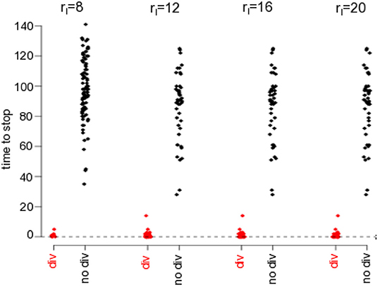
Figure 10. The divergence correlates with the weighted model-observation covariances at observed grid points A_o. The plots show the times of maxima T_o (cf. Equation 37) to stop, i.e., T_stop − T_o. T_o is the time when the mean model-observation covariance A_o is maximum, for divergent (red-colored with break time T_stop) and non-divergent (black colored with maximum time T_stop = 200) trials. Here it is r_H = 5.

Now that A_o is strongly correlated with the filter innovation divergence, the question arises whether the difference between weighted observed and unobserved model-observation covariances is related to the innovation divergence. Figure 11 shows the distribution of A = A_o − A_u and ΔT = T_o − T_u for divergent and non-divergent experimental trials. Most trials exhibit stronger model-observation covariances in unobserved grid points than in observed grid points (A < 0), cf. Figure 11A, and the distribution variances of divergent and non-divergent trials are significantly different (Fligner-Killeen test, p < 0.001). Moreover, the distribution of ΔT in divergent trials is asymmetric since ΔT > 0 for almost all divergent trials (see Figure 11B). Hence weighted model-observation covariances in unobserved grid points reach their maximum significantly earlier than in observed grid points. Conversely, ΔT = 0 of non-divergent trials scatters within a much wider range from negative to positive values (Fligner-Killeen test, p < 0.0001).

FIGURE 11

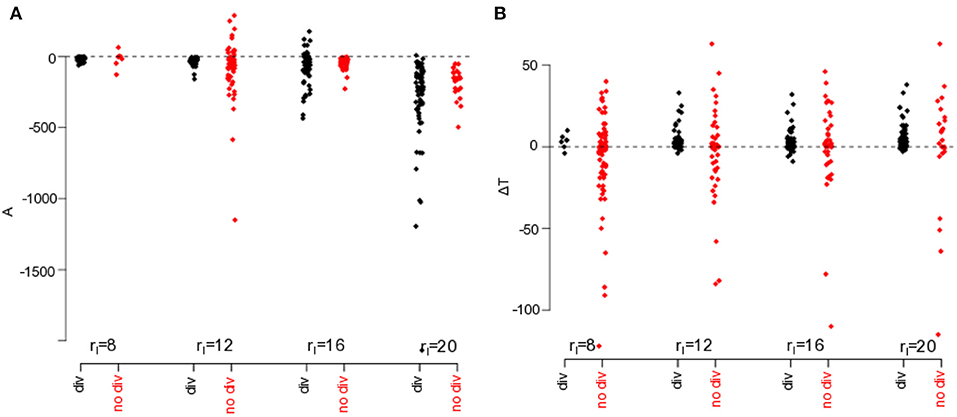
Figure 11. Comparison of weighted model-observation covariances in observed and non-observed grid points. (A) A = A_o − A_u is the difference between maximum weighted model-observation covariances in observed and unobserved grid points. (B) ΔT = T_o − T_u is the difference of times when the weighted model-observation covariances reach their maximum, cf. Equation (38). It is r_H = 5.

In this context, re-call that A_u > A_o but T_u < T_o in divergent trials, i.e., unobserved grid points reach their larger maximum faster than observed grid points. This indicates that the model-observation covariance c_u reflects the instability of the filter.

3.2. Local and Nonlocal Observations

Several international weather services apply ensemble Kalman filters and assimilate both nonlocal and local observations. Performing assimilation experiments similar to the experiments for nonlocal observations but now with a single additional local observation at grid point i = N/2 (cf. section 2.7), the filter divergence rate γ indicates the filter stability. Figure 12 illustrates how local observations affect the filter stability in addition to nonlocal observations. For r_H = 1, the filter diverges rarely due to large innovations (with fewest trials at r_l ≈ 10) but at a larger number than in the absence of local observations, cf. Figure 4. Moreover, increasing the localization radius yields a higher number of trials with catastrophic filter divergence with a maximum catastrophic divergence rate at r_l ≈ 10. In sum, the least number of divergent trials occur at r_l = r_H = 1 (blue curve in Figure 12). A similar stability behavior occurs for r_H = 5 with a minimum innovation divergence rate at r_l ≈ r_H and a maximum catastrophic divergence rate at r_l ≈ 10. Again, the least number of trials diverge at r_l = r_H.

FIGURE 12

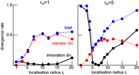
Figure 12. Rate of filter divergence γ (innovation divergence, black line) and catastrophic filter divergence (any ensemble member diverges, red line) in the presence of a single local and a single nonlocal observation. The total number of divergent trials is the sum of innovation and member divergence-trials (blue line). Results are based on 200 numerical trials.

Figure 1 motivates the present work demonstrating that nonlocal observations yield larger first guess departures than for local observations only. Here, it is interesting to note that the numerical trial in Figure 1 with nonlocal observations exceeds the innovation divergence threshold, cf. section 2.8, but has run over all filter cycles for illustration reasons. Moreover, several trials with the same parameters exhibit catastrophic filter divergence and the shown trial is a rare case. This divergence could have been avoided by implementing stabilizing features, such as ensemble enlargement [19], adaptive localization [29], adaptive inflation [18], or first guess check [13, 45]. However, these methods would have introduced additional assimilation effects and the gained results would not have been comparable to findings and insights in the remaining work.

4. Discussion

Ensemble Kalman filtering of nonlocal observations may increase the innovation in the filter process leading to larger observation-background departure bias and RMSE, cf. Figure 1. It is demanding to detect this innovation divergence since it is finite and transient, i.e., of finite duration. At a first glance, this negative impact is surprising since observations are thought to introduce additional knowledge to the system and thus should improve forecasts or at least retain them. To understand better why nonlocal observations may be detrimental, the present work performs numerical studies to identify markers of innovation divergence and understand their origin.

4.1. Nonlocal Observations Facilitate Filter Divergence

The majority of previous stability studies of Kalman filtering involving nonlocal observations consider catastrophic filter divergence. Kelly et al. [20] show analytically for a specific simple but non-trivial model how catastrophic filter divergence of a ensemble Kalman filter is affected by nonlocal observations. The work of Marx and Potthast [44] is an analytical discussion of the linear Kalman filter and the authors derive corresponding stability conditions. Conversely, the present work considers intermittent innovation divergence and, to our best knowledge, is one of the first to demonstrate this important effect numerically. Intermittent innovation divergence is detrimental to forecasts and are visible, e.g., in first guess departure statistics (Figure 1). It occurs for a nonlocal observation only (Figure 4) or for nonlocal and additional local observation (Figure 12). This holds true for almost all localization radii.

4.2. Optimal Localization Radius

Figures 4, 5, 6, 12 show that innovation divergence depends on the relation between sensitivity function width r_H and localization radius r_l. The LETKF diverges least when r_l ≈ r_H and hence this choice of localization radius is called optimal, i.e., the filter is least divergent. This insight agrees with the finding in an operational weather prediction framework involving the LETKF [13]. The authors consider an adaptive localization for (nonlocal) satellite observations and choose the corresponding radius to the sensitivity function width. In two different weather situations, this tight relation improves short- and middle-range weather forecasts compared to the case of independent sensitivity width and localization radius. Figure 9 illustrates the possible reason for the detrimental effect of different sensitivity function width and localization radius: the LETKF is inconsistent if it updates the state at unobserved spatial locations or does not update the state at observed spatial locations. Only if the sensitivity function and the localization width are similar, then this detrimental effect is small. Such an inconsistency is in line with other inconsistencies in ensemble Kalman filters caused by localization, cf. [46]. For instance, a full ensemble reduces inconsistencies for localization radii larger than the sensitivity function width and yields filter stability (Figure 5).

It is important to point out that, under certain conditions, it may be beneficial to further enlarge the localization area compared to the sensitivity function. If the system's activity synchronizes on a larger spatial scale, then information is shared between observed and unobserved grid points and a larger localization radius would be beneficial. Examples for such synchronization phenomena are deep clouds or large-scale winds in meteorology or locally self-organized spots in physical complex systems. In other words, to decide how to choose the localization radius one should take a closer look at the system's dynamics: if larger spatially synchronized phenomena are expected, then r_l ≫ r_H is preferable, otherwise r_l ≈ r_H.

Several previous studies have derived optimal localization radii for local observations in ensemble Kalman filter [47–49] and the specific LETKF [28, 50]. A variant of the LETKF localizes not in observation space as in the present work but in the spatial domain [24, 31, 34, 51], where the localization of nonlocal observations has been studied as well [52]. There is the general agreement for local and nonlocal observations that the optimal localization radius depends on the ensemble size and the observation error but seems to be independent on the model [50].

Essentially, it is important to point out that there may be not a single optimal localization radius but a range of more or less equivalent localization radii. This holds true for smooth localization functions, whereas non-smooth (i.e., unrealistic) localization functions do not show this uncertainty, cf. section 2.4.

4.3. Origin of Divergence

It is important to understand why some numerical trials diverge and some do not. Direct and indirect markers indicate which dynamical features play an important role in divergence. The most obvious direct markers are the absolute values of the innovation and the ensemble member perturbation spread Θ_n and both increase sharply during filter innovation divergence, cf. Figures 4, 6, 7B, 8, 12. Similarly, the covariation of observed and unobserved background errors Ξ_n also increases during divergence. Interestingly, Θ_n and Ξ_n remain finite and take their maxima just before the instance of divergence, cf. Figure 8. The covariation Ξ_n increases if both observed and unobserved errors increases. Kelly et al. [20] and Tong et al. [18] argue that this indicates a shift of power from observed to unobserved errors and that this shift is responsible for catastrophic divergence. The present findings support this line of argumentation and extends it to intermittent innovation divergence. This can be seen in Figure 11A. It shows larger mean weighted model-observation error covariances (i.e., ensemble error covariances) in unobserved grid points than in observed grid points (A < 0) and these weighted model-observation covariances increase faster in unobserved grid points than in observed grid points. In addition, the larger the localization radius r_l > r_H, the larger the ensemble error in unobserved grid points compared to observed grid points. Hence the model-observation covariance reflects a degree of instability (and thus of divergence) in the filter and this is stronger in unobserved grid points than in observed grid points.

Figures 4, 5, 6, 12 provide further evidence on possible error sources that yield filter divergence. The asymmetry of the divergence rates with respect to r_l ≈ r_H hints different underlying filter divergence contributions. If r_l < r_H, too few grid points are updated by the nonlocal observation (Figure 9) although they are observed. Consequently model equivalents in observation space include contributions from non-updated grid points which might yield large contributions to the model equivalents from large model magnitudes and hence this error mechanism is rather strong. Fertig et al. [12] have identified this case as a possible source of divergence and proposed to adapt the localization radius to the sensitivity function width. In fact, this removes case 1 in Figure 9 and stabilizes the filter for r_l < r_H.

For r_l ≫ r_H, a large number of grid points are updated which, however, consider an observation with a large intrinsic error resulting from, e.g., a too small number of ensemble members. The corresponding assimilation error is more subtle than for r_l < r_H and increases for larger localization radii only. The localized nonlocal observation comprises a representation error due to the reduction of the broad sensitivity function to a single location. For small ensembles, this implicit observation error contributes to the analysis update error and, finally, to filter divergence. In sum, the two inconsistencies illustrated in Figure 9 and derived in section 3.1 represent two possible contributions to the filter divergence for a low number of ensemble members. Conversely, for a full ensemble, intrinsic error contributions are well reduced rendering the filter more stable (Figure 5).

Moreover, there is some evidence that ensemble member alignment may cause catastrophic filter divergence [19–21]. Figure 8 shows such indirect markers indicating weak member anti-alignment for r_l ≤ r_H but enhanced alignment and anti-alignment for r_l > r_H. The authors in [19] argue that finite ensemble sizes cause the ensemble to align in case of divergence and Ng et al. [53] show that the ensemble members may align with the most unstable phase space direction. However, our results reveal that member alignment does not represent the major mechanism for innovation divergence. Conversely, Figure 8 provides evidence for alignment of analysis increments and background perturbations when the filter diverges. This alignment indicates that the analysis members point into the same direction as the background members. For instance, if background member perturbations point to less stable locations in phase space, then the LETKF does not correct this direction and the new analysis state is less stable, cf. the model example in [20]. This shows accordance to the reasoning in [53].

In addition to the alignment mechanism, Equation (34) represents the covariation of ensemble perturbations in spatial and observation space at observed and unobserved spatial locations. For observed spatial locations, it is maximum just before the innovation divergence time. Moreover, it reaches its maximum at unobserved locations almost always before the maximum at observed locations are reached (Figure 11). It seems this new feature represent an important contribution to the innovation divergence and future work will analyse this covariation in more detail.

4.4. Limits and Outlook

The present work considers the specific case of finite low ensemble size and application of the localization scheme. To understand better the origin of the filter divergence, it is insightful to study in detail the limiting case of large ensemble sizes, i.e., close to the model dimension, and a neglect of localization. Although this limit is far from practice in seismology and meteorology, where the model systems are too large to study this limit, nevertheless this limit study is of theoretical interest and future work will consider it in some detail.

There is some evidence that the optimal localization radius is flow-dependent [54, 55], whereas we assume a constant radius. In addition, the constrained choice of parameters and missing standard techniques to prevent divergence, such as adaptive inflation and adaptive observation error, limits the present work in generality and interpretation and thus makes it hard to derive decisive conclusions. Future work will implement adaptive schemes [56, 57] in a more realistic model framework.

In the majority of studies, the present work considers a non-smooth boxcar sensitivity function in order to distinguish observed and unobserved grid points. Although this simplification allows to gain deeper understanding of possible contributions to the filter divergence, the sensitivity function is unrealistic. A more realistic sensitivity function is smooth and unimodal or bimodal. Figure 5 shows that such a sensitivity function yields a minimum divergence rate but the localization radius at the minimum rate is much smaller than the sensitivity function width. Consequently, the line of argumentation about Figure 9 does not apply here since there is no clear distinction of observed and unobserved grid points anymore. Future work will attempt to consider smooth unimodal sensitivity functions.

Moreover, the localization scheme of nonlocal observations applied in the present work is very basic due to its choice of the maximum sensitivity as the observations location. Future work will investigate cut-off criteria as such in [12] that chooses the location of nonlocal observations in the range of the sensitivity function. Fertig et al. [12] also have shown that such a cut-off criterion improves first guess departure statistics and well reduces the divergence for localization radii that are smaller than the sensitivity weighting function.

Nevertheless the present work introduces the problem of intermittent innovation divergence, extends lines of reason on the origin of filter divergence to nonlocal observation and proposes new markers of innovation divergence.

Data Availability Statement

The datasets generated for this study are available on request to the corresponding author.

Author Contributions

AH conceived the work, performed all simulations, and wrote the manuscript.

Conflict of Interest

The author declares that the research was conducted in the absence of any commercial or financial relationships that could be construed as a potential conflict of interest.

Acknowledgments

AH would like to thank Roland Potthast for insightful hints on the stability of Kalman filters. Moreover, the author very much appreciates the valuable comments of the reviewers, whose various insightful comments helped very much to improve the manuscript.

References

1. Bengtsson L, Ghil M, Källén E, . (eds). Dynamic Meteorology: Data Assimilation Methods, Applied Mathematical Sciences. Vol. 36. New York, NY: Springer (1981).

Google Scholar

2. Luo X, Bhakta T, Jakobsen M, Navdal G. Efficient big data assimilation through sparse representation: a 3D benchmark case study in petroleum engineering. PLoS ONE (2018) 13:e0198586. doi: 10.1371/journal.pone.0198586

PubMed Abstract | CrossRef Full Text | Google Scholar

3. Hutt A, Stannat W, Potthast R, . (eds.). Data Assimilation and Control: Theory and Applications in Life Sciences. Lausanne: Frontiers Media (2019).

Google Scholar

4. Schiff SJ. Neural Control Engineering. Cambridge, MA: MIT Press (2011).

Google Scholar

5. Nakamura G, Potthast R. Inverse Modeling. Bristol: IOP Publishing (2015).

Google Scholar

6. Asch M, Bocquet M, Nodet M. Data Assimilation: Methods, Algorithms, and Applications. Philadelphia, PA: SIAM (2016).

Google Scholar

7. Hunt B, Kostelich E, Szunyoghc I. Efficient data assimilation for spatiotemporal chaos: a local ensemble transform Kalman filter. Phys D. (2007) 230:112–26. doi: 10.1016/j.physd.2006.11.008

CrossRef Full Text | Google Scholar

8. Schraff C, Reich H, Rhodin A, Schomburg A, Stephan K, Perianez A, et al. Kilometre-scale ensemble data assimilation for the cosmo model (kenda). Q J R Meteorol Soc. (2016) 142:1453–72. doi: 10.1002/qj.2748

CrossRef Full Text | Google Scholar

9. Schomburg A, Schraff C, Potthast R. A concept for the assimilation of satellite cloud information in an ensemble Kalman filter: single-observation experiments. Q J R Meteorol Soc. (2015) 141:893–908. doi: 10.1002/qj.2748

CrossRef Full Text | Google Scholar

10. Miyoshi T, Sato Y. Assimilating satellite radiances with a local ensemble transform Kalman filter (LETKF) applied to the JMA global model (GSM). SOLA. (2007) 3:37–40. doi: 10.2151/sola.2007-010

CrossRef Full Text | Google Scholar

11. Kurzrock F, Cros S, Ming F, Otkin J, Hutt A, Linguet L, et al. A review of the use of geostationary satellite observations in regional-scale models for short-term cloud forecasting. Meteorol Zeitsch. (2018) 27:277–98. doi: 10.1127/metz/2018/0904

CrossRef Full Text | Google Scholar

12. Fertig EJ, Hunt BR, Ott E, Szunyogh I. Assimilating non-local observations with a local ensemble Kalman filter. Tellus A. (2007) 59:719–30. doi: 10.1111/j.1600-0870.2007.00260.x

CrossRef Full Text | Google Scholar

13. Hutt A, Schraff C, Anlauf H, Bach L, Baldauf M, Bauernschubert E, et al. Assimilation of SEVIRI water vapour channels with an ensemble Kalman filter on the convective scale. Front Earth Sci. (2019) 8:70. doi: 10.3389/feart.2020.00070

CrossRef Full Text | Google Scholar

14. Furrer R, Bengtsson T. Estimation of high-dimensional prior and posterior covariance matrices in Kalman filter variants. J Multivar Anal. (2007) 98:227–55. doi: 10.1016/j.jmva.2006.08.003

CrossRef Full Text | Google Scholar

15. Anderson JL. An ensemble adjustment Kalman filter for data assimiliation. Mon Weather Rev. (2001) 129:2884–903. doi: 10.1175/1520-0493(2001)129<2884:AEAKFF>2.0.CO;2

CrossRef Full Text | Google Scholar

16. Hamill TM, Whitaker JS, Snyder C. Distance-dependent filtering of background error covariance estimates in an ensemble Kalman filter. Mon Weather Rev. (2001) 129:2776–90. doi: 10.1175/1520-0493

CrossRef Full Text | Google Scholar

17. Tong XT, Majda A, Kelly D. Nonlinear stability and ergodicity of ensemble based Kalman filters. Nonlinearity. (2016) 29:657–91. doi: 10.1088/0951-7715/29/2/657

CrossRef Full Text | Google Scholar

18. Tong XT, Majda A, Kelly D. Nonlinear stability of ensemble Kalman filters with adaptive covariance inflation. Commun Math Sci. (2016) 14:1283–313. doi: 10.4310/cms.2016.v14.n5.a5

CrossRef Full Text | Google Scholar

19. Gottwald G, Majda AJ. A mechanism for catastrophic filter divergence in data assimilation for sparse observation networks. Nonlin Process Geophys. (2013) 20:705–12. doi: 10.5194/npg-20-705-2013

CrossRef Full Text | Google Scholar

20. Kelly D, Majda A, Tong XT. Concrete ensemble Kalman filters with rigorous catastrophic filter divergence. Proc Natl Acad Sci USA. (2015) 112:10589–94. doi: 10.1073/pnas.1511063112

PubMed Abstract | CrossRef Full Text | Google Scholar

21. Majda A, Harlim J. Catastrophic filter divergence in filtering nonlinear dissipative systems. Commun Math Sci. (2008) 8:27–43. doi: 10.4310/CMS.2010.v8.n1.a3

CrossRef Full Text | Google Scholar

22. Migliorini S, Candy B. All-sky satellite data assimilation of microwave temperature sounding channels at the met office. Q J R Meteor Soc. (2019) 145:867–83. doi: 10.1002/qj.3470

CrossRef Full Text | Google Scholar

23. Lorenz EN, Emanuel KA. Optimal sites for supplementary weather observations: simulations with a small model. J Atmos Sci. (1998) 555:399–414. doi: 10.1175/1520-0469(1998)055<0399:SFSWO>2.0.CO;2

CrossRef Full Text | Google Scholar

24. Bishop CH, Whitaker JS, Lei L. Gain form of the Ensemble Transform Kalman Filter and its relevance to satellite data assimilation with model space ensemble covariance localization. Mon Weather Rev. (2017) 145:4575–92. doi: 10.1175/MWR-D-17-0102.1

CrossRef Full Text | Google Scholar

25. Gaspari G, Cohn S. Construction of correlation functions in two and three dimensions. Q J R Meteorol Soc. (1999) 125:723–57.

Google Scholar

26. Waller JA, Dance SL, Lawless AS, Nichols NK. Estimating correlated observation error statistics using an ensemble transform Kalman filter. Tellus A. (2014) 66:23294. doi: 10.3402/tellusa.v66.23294

CrossRef Full Text | Google Scholar

27. Houtekamer PL, Zhang F. Review of the ensemble Kalman filter for atmospheric data assimilation. Mon Weather Rev. (2016) 144:4489–532. doi: 10.1175/MWR-D-15-0440.1

CrossRef Full Text | Google Scholar

28. Perianez A, Reich H, Potthast R. Optimal localization for ensemble Kalman filter systems. J Met Soc Jpn. (2014) 92:585–97. doi: 10.2151/jmsj.2014-605

CrossRef Full Text | Google Scholar

29. Greybush SJ, Kalnay E, Miyoshi T, Ide K, Hunt BR. Balance and ensemble Kalman filter localization techniques. Mon Weather Rev. (2011) 139:511–22. doi: 10.1175/2010MWR3328.1

CrossRef Full Text | Google Scholar

30. Nadeem A, Potthast R. Transformed and generalized localization for ensemble methods in data assimilation. Math Methods Appl Sci. (2016) 39:619–34. doi: 10.1002/mma.3496

CrossRef Full Text | Google Scholar

31. Bishop CH, Hodyss D. Ensemble covariances adaptively localized with eco-rap. Part 2: a strategy for the atmosphere. Tellus. (2009) 61A:97–111. doi: 10.1111/j.1600-0870.2008.00372

CrossRef Full Text | Google Scholar

32. Leng H, Song J, Lu F, Cao X. A new data assimilation scheme: the space-expanded ensemble localization Kalman filter. Adv Meteorol. (2013) 2013:410812. doi: 10.1155/2013/410812

CrossRef Full Text | Google Scholar

33. Miyoshi T, Yamane S. Local ensemble transform Kalman filtering with an AGCM at a T159/L48 resolution. Mon Weather Rev. (2007) 135:3841–61. doi: 10.1175/2007MWR1873.1

CrossRef Full Text | Google Scholar

34. Farchi A, Boquet M. On the efficiency of covariance localisation of the ensemble Kalman filter using augmented ensembles. Front Appl Math Stat. (2019) 5:3. doi: 10.3389/fams.2019.00003

CrossRef Full Text

35. Lei L, Whitaker JS. Model space localization is not always better than observation space localization for assimilation of satellite radiances. Mon Weather Rev. (2015) 143:3948–55. doi: 10.1175/MWR-D-14-00413.1

CrossRef Full Text | Google Scholar

36. Campbell WF, Bishop CH, Hodyss D. Vertical covariance localization for satellite radiances in ensemble Kalman filters. Mon Weather Rev. (2010) 138:282–90. doi: 10.1175/MWR3017.1

CrossRef Full Text | Google Scholar

37. Houtekamer PL, Mitchell H, Pellerin G, Buehner M, Charron M, Spacek L, et al. Atmospheric data assimilation with an ensemble Kalman filter: results with real observations. Mon Weather Rev. (2005) 133:604–20. doi: 10.1175/MWR-2864.1

CrossRef Full Text | Google Scholar

38. Higham NJ. Accuracy and Stability of Numerical Algorithms. 2nd Edn. Philadelphia, PA: SIAM (2002).

Google Scholar

39. Anderson JL, Anderson SL. A monte carlo implementation of the nonlinear filtering problem to produce ensemble assimilations and forecasts. Mon Weather Rev. (1999) 127:2741–58. doi: 10.1175/1520-0493.

CrossRef Full Text | Google Scholar

40. Luo X, Hoteit I. Covariance inflation in the ensemble Kalman filter: a residual nudging perspective and some implications. Mon Weather Rev. (2013) 141:3360–8. doi: 10.1175/MWR-D-13-00067.1

CrossRef Full Text | Google Scholar

41. Hamill TM, Whitaker JS. What constrains spread growth in forecasts initialized from ensemble Kalman filters ? Mon Weather Rev. (2011) 139:117–31. doi: 10.1175/2010MWR3246.1

CrossRef Full Text | Google Scholar

42. Mitchell HL, Houtekamer PL. An adaptive ensemble Kalman filter. Mon Weather Rev. (2000) 128:416–33. doi: 10.1175/1520-0493

CrossRef Full Text | Google Scholar

43. Grewal MS, Andrews AP. Kalman Filtering: Theory and Practice Useing MATLAB. 2nd Edn. Hoboken, NJ: John Wiley & Sons (2001).

Google Scholar

44. Marx B, Potthast R. On instabilities in data assimilation algorithms. Mathematics. (2012) 8:27–43. doi: 10.1007/s13137-012-0034-5

CrossRef Full Text | Google Scholar

45. Lahoz WA, Schneider P. Data assimilation: making sense of earth observation. Front Environ Sci. (2014) 2:16. doi: 10.3389/fenvs.2014.00016

CrossRef Full Text | Google Scholar

46. Tong XT. Performance analysis of local ensemble Kalman filter. J Nonlin Sci. (2018) 28:1397–442. doi: 10.1007/s00332-018-9453-2

CrossRef Full Text | Google Scholar

47. Ying Y, Zhang F, Anderson J. On the selection of localization radius in ensemble filtering for multiscale quasigeostrophic dynamics. Mon Weather Rev. (2018) 146:543–60. doi: 10.1175/MWR-D-17-0336.1

CrossRef Full Text | Google Scholar

48. Miyoshi T, Kondo K. A multi-scale localization approach to an ensemble Kalman filter. SOLA. (2013) 9:170–3. doi: 10.2151/sola.2013-038

CrossRef Full Text | Google Scholar

49. Migliorini S. Information-based data selection for ensemble data assimilation. Q J R Meteorol Soc. (2013) 139:2033–54. doi: 10.1002/qj.2104

CrossRef Full Text | Google Scholar

50. Kirchgessner P, Nerger L, Bunse-Gerstner A. On the choice of an optimal localization radius in Ensemble Kalman Filter methods. Mon Weather Rev. (2014) 142:2165–75. doi: 10.1175/MWR-D-13-00246.1

CrossRef Full Text | Google Scholar

51. Bishop CH, Whitaker JS, Lei L. Commentary: On the efficiency of covariance localisation of the ensemble Kalman filter using augmented ensembles by alban farchi and marc bocquet. Front Appl Math Stat. (2020) 6:2. doi: 10.3389/fams.2020.00002

CrossRef Full Text | Google Scholar

52. Lei L, Whitaker JS, Bishop C. Improving assimilation of radiance observations by implementing model space localization in an ensemble Kalman filter. J Adv Model Earth Syst. (2018) 10:3221–32. doi: 10.1029/2018MS001468

CrossRef Full Text | Google Scholar

53. Ng GHC, McLaughlin D, Entekhabi D, Ahanin A. The role of model dynamics in ensemble Kalman filter performance for chaotic systems. Tellus A. (2011) 63:958–77. doi: 10.1111/j.1600-0870.2011.00539.x

CrossRef Full Text | Google Scholar

54. Zhen Y, Zhang F. A probabilistic approach to adaptive covariance localization for serial ensemble square root filters. Mon Weather Rev. (2014) 142:4499–518. doi: 10.1175/MWR-D-13-00390.1

CrossRef Full Text | Google Scholar

55. Flowerdew J. Towards a theory of optimal localisation. Tellus A. (2015) 67:25257. doi: 10.3402/tellusa.v67.25257

CrossRef Full Text | Google Scholar

56. Lee Y, Majda AJ, Qi D. Preventing catastrophic filter divergence using adaptive additive inflation for baroclinic turbulence. Mon Weather Rev. (2017) 145:669–82. doi: 10.1175/MWR-D-16-0121.1

CrossRef Full Text | Google Scholar

57. Miyoshi T. The gaussian approach to adaptive covariance inflation and its implementation with the local ensemble transform Kalman filter. Mon Weather Rev. (2011) 139:1519–35. doi: 10.1175/2010MWR3570.1

CrossRef Full Text | Google Scholar