The Construction of Efficient Portfolios: A Verification of Risk Models for Investment Making

Introduction

In this paper, we study the construction of US mean-variance efficient portfolios during the period 1999–2017. We construct mean-variance portfolios by maximizing the 10-factor U.S. Expected Return stock selection model (USER) alphas and constraining Tracking Error with respect to the S&P 500 benchmark using 3-factor risk model of Blume et al. [1]¹. The main finding of this paper is that the mean-variance efficient portfolios produce statistically significant portfolio excess returns in the US market.

The organization of the paper is as follows. The first section describes the construction of efficient portfolios, estimation of covariance matrix with multi-factor models, and the data used in construction of size ranked portfolios in estimating common risk factors. The second section describes the expected excess return model used in the study, statistical estimation method, and the data. The third section describes construction of tracking portfolios and presents portfolio statistics. The final section contains concluding remarks.

Constructing Efficient Portfolios

The Markowitz portfolio construction approach is based on the premise that mean and variance of future outcomes are sufficient for rational decision making under uncertainty, to identify the best opportunity set, efficient frontier, where returns are maximized for a given level of risk, or minimize risk for a given level of return. The reader is referred to Markowitz [14, 15] for the seminal discussion of portfolio construction and management. The two parameters needed are the portfolio expected return, E(R_p) is calculated by taking the sum of the security weights, w multiplied by their respective expected returns, and the portfolio standard deviation is the sum of the weighted covariances.

$\begin{array}{ll}{\mu }_P=E^{T}W& (1)\end{array}$

$\begin{array}{ll}{\sigma }_P^2=W^T\Omega W& (2)\end{array}$

$\begin{array}{ll}{W}^T\underset{\_}{1}=1& (3)\end{array}$

where, E = {μ₁, μ₂,…,μ_N} is N × 1 vector of expected security returns, (N is the number of candidate securities), Ω is the N × N covariance matrix, W = {w₁, w₂,…, w_N} is the vector of weights, and 1 is the unit column vector. Sum of weights in (3) indicates that the portfolio is fully invested.

One can construct infinite number of Mean-Variance efficient portfolios. Optimal portfolio choice decision will be determined by an investors' risk tolerance². Following Markowitz's [14, 16–18] general portfolio optimization objective function is:

$\begin{array}{ll}Min{W}^T\Omega W-\lambda E^{T}W& (4)\end{array}$

where, λ is the coefficient of relative risk aversion of the investor³.

Accurate characterization of portfolio risk requires an accurate estimate of the covariance matrix of security returns.

Estimation of the covariance structure is almost always based on a linear return generating multi-factor model (MFM) in the form of:

$\begin{array}{ll}{\text{R}}_{\text{j,t}}={\displaystyle \sum _{\text{k }=1}^{\text{K}}}{\beta }_{\text{jk}}{\tilde{\text{f}}}_{\text{k,t}}+{\tilde{\text{e}}}_{\text{j,t}}& (5)\end{array}$

The non-factor, or asset-specific return on security j ${\tilde{\text{e}}}_{\text{j,t}}$ is the residual return of the security after removing the estimated impacts of the finite number of K factors where 1 ≤ K ≤ N. The term ${\tilde{\text{f}}}_{\text{k,t}}$ is the rate of return of factor “k,” which is independent of securities and affects the security's return through its exposure coefficient β_jk. Under the assumption that the residual return e_j,t is not correlated across securities the covariance matrix of the securities is reduced to form:

$\begin{array}{ll}\Omega =B^T\Theta \text{B+}{\rm Y}& (6)\end{array}$

$\begin{array}{l}\text{ where:}\\ B_{k\times N}=\left(\begin{array}{cccc}{\beta }_{1,1}& {\beta }_{1,2}& \cdots & {\beta }_{1,N}\\ {\beta }_{2,1}& {\beta }_{2,2}& \cdots & {\beta }_{2,N}\\ ⋮& ⋮& \cdots & ⋮\\ {\beta }_{k,1}& {\beta }_{k,2}& \cdots & {\beta }_{k,N}\end{array}\right)& (7)\end{array}$

$\begin{array}{ll}{\Theta }_{k\times k}=\left(\begin{array}{cccc}{\sigma }_{f_1,f_1}& {\sigma }_{f_1,f_2}& \cdots & {\sigma }_{f_1,f_k}\\ {\sigma }_{f_2,f_1}& {\sigma }_{f_2,f_2}& \cdots & {\sigma }_{f_2,f_k}\\ ⋮& ⋮& \cdots & ⋮\\ {\sigma }_{f_k,f_1}& {\sigma }_{f_k,f_1}& \cdots & {\sigma }_{f_k,f_k}\end{array}\right)& (8)\end{array}$

$\begin{array}{ll}{{\rm Y}}_{N\times N}=\left(\begin{array}{cccc}{\sigma }_{e_1}^2& 0& \cdots & 0\\ 0& {\sigma }_{e_2}^2& \cdots & 0\\ ⋮& ⋮& \cdots & ⋮\\ 0& 0& \cdots & {\sigma }_{e_N}^2\end{array}\right)& (9)\end{array}$

B in (7) is the matrix of exposure coefficients, also referred as “loadings” in the literature, θ in (8) is the covariance matrix of the factors, and ⋎ in (9) is the covariance of the residuals.

The very first model used in the literature is Treynor's market model that led to development of the Capital Asset Pricing Model (CAPM)⁴. There is a rich volume of research covering multi factor models starting with King [4].

In this paper, we use a statistical risk model developed by Blume et al. [1], (BGG). Statistical factor models deduce the appropriate factor structure by analyzing the sample asset returns covariance matrix. There is no need to pre-define factors and compute exposures, as required by fundamental factor models. The only inputs are a time-series of asset returns and the number of desired factors. BGG has shown that return generating model based on factors analysis estimation is superior to commonly used multi-factor models used in the literature.

Data and Estimation Methodology

The empirical analyses to estimate the factors use monthly returns of 444 sets of size-ranked portfolios of NYSE stocks constructed from the CRSP file. The first set consists of all securities in the CRSP files with complete data for the 5 years 1980 through 1984. These securities ranked by their market value as of December 1979 and then partitioned into 30 equally weighted size-ranked portfolios with as close to an equal number of securities as possible. This process is repeated for each rolling 5-year period every month to December 2017 with each set consisting 30 monthly portfolio returns with 60 observations.

We use the maximum likelihood method (MLM) to estimate the factor models; the usual way to assess the number of required factors is to rerun the procedure, successively increasing the number of factors until the X² test for the goodness of fit developed by Bartlett [25] indicates that the number of factors is generally shown to be sufficient in explaining returns. To use this criterion, one must specify the level of significance, often arbitrarily set at 1 or 5 percent. The level of significance is important since there is a direct relation between the level of significance and the number of significant factors. BGG's findings indicate that the number of required factors varies over time. Their analysis of the required number of factors reveals a positive relation between the number of factors and the variability of returns during the estimation period. A rationale for this finding is that during periods of relatively low volatility, most of the volatility is firm specific and it is difficult to identify the common factors. In more volatile times, the common factors are relatively more important than the firm-specific factors, making it easier to identify them. Their findings indicate that median number of factor required to explain the returns at 5 percent confidence level is three. In Figure 1 we plot the standard deviation of portfolio 1, (small cap), portfolio 30, (large-cap), and the number of factors required at 5 percent confidence level. The number of factors needed during the study period is between two and four. In this paper, we set the number of factors to three rather than varying them over time based on Bartlett's goodness of fit criteria.

FIGURE 1

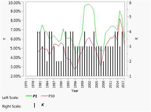
Figure 1. Optimum number of factors and standard deviation of portfolio 1 & 30.

For each security in our universe and the benchmark (S&P 500), we estimated the factor loadings over the same period in (5) with three factors extracted from 30 size ranked portfolio returns. We then estimated the covariance matrix for each month, based on the previous 5 years of monthly data for the securities in our universe and the benchmark as:

$\begin{array}{l}{\stackrel{⌢}{\Omega }}_{t,NxN}\cong B_{t,kxN}^T{B}_{t,kxN}\\ \text{Where}\\ B_{t,kxN}=\left(\begin{array}{cccc}{\stackrel{⌢}{\beta }}_{t,1,1}& {\stackrel{⌢}{\beta }}_{t,1,2}& \cdots & {\stackrel{⌢}{\beta }}_{t,1,k}\\ {\stackrel{⌢}{\beta }}_{t,2,1}& {\stackrel{⌢}{\beta }}_{t,2,2}& \cdots & {\stackrel{⌢}{\beta }}_{t,2,k}\\ ⋮& ⋮& \cdots & ⋮\\ {\stackrel{⌢}{\beta }}_{t,N,1}& {\stackrel{⌢}{\beta }}_{t,N,2}& \cdots & {\stackrel{⌢}{\beta }}_{t,N,k}\end{array}\right)& (10)\end{array}$

Note that the MLM estimation extracts orthogonal factors and the variance of the factors is set to unity by default. That is, Ψ in (9) is reduced to N × N unit matrix. In this paper we assume that factor loadings are stationary over the month (B_{t+1, k} = B_t,k) in estimating the weight of each security in tracking portfolio.

Estimation of Expected Returns

There are many approaches to security valuation and the creation of expected returns. We believe that asset managers use security analysis and stock selection models consisting of reported earnings, forecasted earnings and financial data⁵. Graham and Dodd [27] recommended that stocks be purchased on the basis of the price-earnings (P/E) ratio. The “low” PE investment strategy was discussed in Williams [28], the monograph that influenced Harry Markowitz and his thinking on portfolio construction. Bloch et al. [29] and Haugen and Baker [30, 31] advocated models incorporating earnings-to-price (EP), book-value-to-price, BP, cash flow-to-price, CP, sales-to-price, SP, and other fundamental data. Guerard et al. [32, 33] added price momentum (PM), price at t-1 divided by the price 12 months ago, t-12, and consensus temporary earnings forecast (CTEF) to expected returns modeling. They denoted the stock selection model as United States Expected Returns (USER). They reported, among other results, that: (1) the EP variable had a larger average weight than the BP variable; (2) the relative PE, denoted RPE, the EP relative to its 60-month average had a higher average weight than the PE variable; and (3) the composite earnings forecast variable, CTEF, had a larger weight than the RPE variable. In fact, in the USER model, only the price momentum variable, PM, had a higher weight than the CTEF variable (and only by one percent, at that)⁶.

In this paper, we use the same USER Model.

$\begin{array}{l}\text{ T}{\text{R}}_{\text{t}+1}={\text{a}}_0+{\text{a}}_1\text{E}{\text{P}}_{\text{t}}+{\text{a}}_2\text{B}{\text{P}}_{\text{t}}+{\text{a}}_3\text{C}{\text{P}}_{\text{t}}+{\text{a}}_4\text{S}{\text{P}}_{\text{t}}+{\text{a}}_5\text{RE}{\text{P}}_{\text{t}}\\ +{\text{a}}_6\text{RB}{\text{P}}_{\text{t}}+{\text{a}}_7\text{RC}{\text{P}}_{\text{t}}+{\text{a}}_8\text{RS}{\text{P}}_{\text{t}}+{\text{a}}_9\text{CTE}{\text{F}}_{\text{t}}+{\text{a}}_{10}\text{P}{\text{M}}_{\text{t}}+{\text{e}}_{\text{t}}& (11)\end{array}$

$\begin{array}{l}\text{where}:\text{ EP}=[\text{earnings per share}]/[\text{price per share}]\\ =\text{earnings}-\text{price ratio};\\ \text{ BP}=[\text{book value per share}]/[\text{price per share}]\\ =\text{book}-\text{price ratio};\\ \text{ CP}=[\text{cash flow per share}]/[\text{price per share}]\\ =\text{ cash flow}-\text{price ratio};\\ \text{ SP}=[\text{net sales per share}]/[\text{price per share}]\\ =\text{sales}-\text{price ratio};\\ \text{ REP}=[\text{current EP ratio}]/[\text{average EP ratio over}\\ \text{ the past 5 years}];\\ \text{ RBP}=[\text{current BP ratio}]/[\text{average BP ratio over}\\ \text{ the past 5 years}];\\ \text{ RCP}=[\text{current CP ratio}]/[\text{average CP ratio over}\\ \text{ the past 5 years}];\\ \text{ RSP}=[\text{current SP ratio}]/[\text{average SP ratio over}\\ \text{ the past 5 years}];\\ \text{ CTEF}=\text{consensus earnings}-\text{per}-\text{share}\\ \text{ I/B/E/S forecast},\text{ revisions},\text{ and breadth},\\ \text{ PM}=\text{Price Momentum};\\ \text{ e}=\text{randomly distributed error term}.\end{array}$

Given concerns about both outlier distortion and multicollinearity, Bloch et al. [29] tested the relative explanatory and predictive merits of alternative regression estimation procedures: OLS, robust regression using the Beaton and Tukey [42] bi-square criterion to mitigate the impact of outliers, latent root to address the issue of multicollinearity [see [43]], and weighted latent root, denoted WLRR, a combination of robust and latent root. The Guerard et al. [33] USER model test substantiated the Bloch et al. [29] approach, techniques, and conclusions that WLLR works best among the alternative linear predictive models.

Data and Estimation

For each security, we use monthly total stock returns and prices from CRSP files, earnings book value cash flow, net sales from quarterly COMPUSTAT files, and consensus earnings-per-share, forecast revisions and breadth from I/B/E/S files. We construct the variables used in (8) for each month starting in January 1980. The USER model is estimated using WLRR analysis over the 60 month (5 year) moving window for each period to identify variables statistically significant at the 10% level. The model uses the normalized coefficients as weights over the past 12 months with Beaton-Tukey outlier adjustment. We use the statistically significant coefficients to estimate the next month's expected return rank, E_i, for each security. The USER estimation conditions are virtually identical to those described in Guerard et al. [32, 33, 44].

Portfolio Construction

We construct monthly long only, i.e., w_i ≥ 0, portfolios to track S&P 500 index with minimum tracking error by solving the following equation:

$\begin{array}{l}\text{Min }{W}_t^T\stackrel{⌢}{\Omega }{W}_t-\lambda E_t^T{W}_t-{\stackrel{⌢}{\sigma }}_{S\&P500,t}^2+Z_{t}c\\ st:\\ W_t^T\underset{\_}{1}=1\\ X_t^T\underset{\_}{1}\le M\\ Z_t\underset{\_}{1}\le M\times p\\ x_{i,t}=(\begin{array}{l}1,for{w}_{i,t}>0\hfill \\ 0,\text{ for }{w}_{i,t}=0\hfill \end{array}\\ w_{i,t}\ge 0,i=1,\cdots ,N& (12)\end{array}$

where λ is the relative risk aversion, $\underset{-}{1}$ is the unit, vector X_t = {x_1,t, x_{2, t}, …, x_N,t} is the vector of binary variables that indicate if the security i is included in the portfolio in month t, Z_t = {|x_{1, t} − x_{1, t−1}|, |x_{2, t} − x_{2, t−1}|, …, |x_{N, t} − x_{N, t−1}|} is the vector of binary variables to account for security turnover, c is the transaction cost, p is the portfolio turnover limit percentage, and M is the maximum number of securities allowed in the portfolio. Variance of S&P 500 for the period in Equation (12) is estimated with Equation (10) using the factor loadings of the 3-factor model. We specifically solve Equation (12) with a relatively small number of securities (M), set at 50 and 100 or less, transactions cost (c), set 150 basis points each way, and portfolio turnover (p) set at 8 percent or less⁷.

In Table 1, we present portfolio statistics for each year for relative risk aversion of 0.01, 0.05, and 0.10. Excess return is the annual portfolio return net of truncations costs in excess of the annual return of S&P 500. Relative Sharpe ratios is portfolio Sharpe ratio divided by Share ratio of S&P 500. The active average excess returns of the USER model are statistically significant. Tracking error is not statistically significant for 100-security portfolio.

TABLE 1

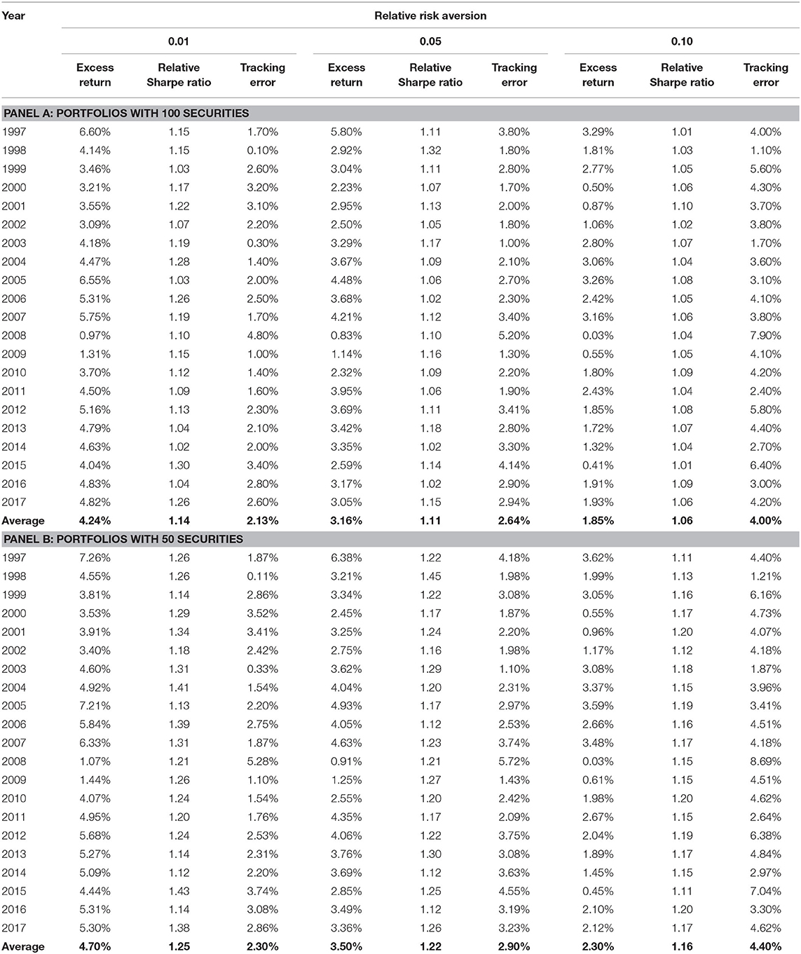
Table 1. Portfolio Statistics for the USER model.

Summary and Conclusions

Investing with fundamental, expectations, and momentum variables is a good investment strategy over the long run. The use of multi-factor risk-control significantly improves portfolios performance relative to the benchmark. We considered long only portfolio construction in this study. Construction of realistic Long–Short portfolios are not feasible under these settings unless one assumes that securities are always available to borrow to short sell. However, there are various actively traded derivative securities based on S&P 500 index, the benchmark used in this study. Portfolios constructed in the study tracks the S&P Index with reasonably low tracking error. With the use of these derivative securities, it is possible to expand the opportunity set for investors.

Data Availability Statement

The raw data supporting the conclusions of this article will be made available by the authors, without undue reservation, to any qualified researcher.

Author Contributions

All authors listed have made a substantial, direct and intellectual contribution to the work, and approved it for publication.

Conflict of Interest

JG is employed by company McKinley Capital Management, LLC.

The remaining authors declare that the research was conducted in the absence of any commercial or financial relationships that could be construed as a potential conflict of interest.

Acknowledgments

We thank the referees for their helpful comments and recommendations.

Footnotes

1. ^An assumption underlying many studies is that the market model, or more generally a model with one factor common to all securities, generates realized returns. In such a one-factor model, realized returns are the sum of an asset's response to a stochastic factor common to all assets and a factor unique to the individual asset. In the last decade, there has been much interest in models with more than one common stochastic factor, using either pre-specified factors, like Fama and French [2] 3-factor model, or factors identified through factor analysis or similar multivariate techniques. Factor analysis and similar factor analytic techniques have on occasion played an important role in the analysis of returns on common stocks and other types of financial assets. Farrar [3] may have been the first to use factor analysis in conjunction with principal component analysis to assign securities into homogeneous correlation groups. King [4] used factor analysis to evaluate the role of market and industry factors in explaining stock returns. These two studies sparked an interest in multi-index models, and a rich body of empirical work soon emerged. Examples include Elton and Gruber [5, 6], Meyer [7], Farrell [8], and Livingston [9], among others. The major goal of these earlier studies was to establish the smallest number of “indexes” needed to construct efficient sets. Factor models have been used in the tests of arbitrage pricing theory and its variants. See for example, Ross and Roll [10] and Dhrymes et al. [11–13], to cite a few from the large literature.

2. ^This is the well know Separation Theorem in the economic theory. Opportunity set is independent of individuals' preferences.

3. ^A rich and detailed Mean-Variance portfolio construction methods are covered in Elton et al. [19] and Rudd and Rosenberg [20].

4. ^There is a rich literature related to CAPM. Treynor's equilibrium model based on the market model in an unpublished internal memorandum is most likely the first one. CAPM is attributed to works of Sharpe [21], Lintner [22], and Mossin [23]. For a very detailed analysis of CAPM, see Mossin [24].

5. ^Expected earnings have been used as a proxy for company's future cash flow in many studies. For a detailed analysis of analysts' consensus forecasts and share prices, see Elton et al. [26].

6. ^Wall Street practitioners have embraced the “low PE” approach for well over 50 years. The low PE strategy is a form of the contrarian investment approach associated with Bernard [34] and Dremen [35, 36]. The authors believe in the low PE strategy, but not as the exclusive strategy. There is extensive literature on the impact of individual value ratios on the cross section of stock returns. We go beyond using just one or two of the standard value ratios (EP and BP) to include the cash-price ratio (CP) and/or the sales-price ratio (SP). Several major papers on combination of value ratios to predict stock returns (that include at least CP and/or SP) are Fama and French [2, 37, 38], Bloch et al. [29], Chan et al. [39], Blin et al. [40], Guerard, Gültekin, and Stone [41], and Haugen and Baker [30, 31].

7. ^The second constraint in (12) was binding at all months.

References

1. Blume M, Gültekin MN, Gültekin NB. Validating return-generating models. In: Guerard JG, editor. Portfolio Construction, Measurement, and Efficiency: Essays in Honor of Jack Treynor. Springer (2017). p. 111–34. doi: 10.1007/978-3-319-33976-4_5

CrossRef Full Text | Google Scholar

2. Fama EF, French KR. Cross-sectional variation in expected stock returns. J Finance. (1992) 47:427–65. doi: 10.1111/j.1540-6261.1992.tb04398.x

CrossRef Full Text

3. Farrar DE. The Investment Decision Under Uncertainty. Englewood Cliffs, NJ: Prentice-Hall, Inc. (1962).

4. King BF. Market and industry factors in stock price behavior. J Business. (1966) 39:139–90. doi: 10.1086/294847

CrossRef Full Text | Google Scholar

5. Elton EJ, Gruber MJ. Dynamic programming applications in finance. J Finance. (1971) 26:473–506.

Google Scholar

6. Elton EJ, Gruber MJ. Estimating the dependence structure of share prices–implications for portfolio selection. J Finance. (1973) 28:1203–32.

Google Scholar

7. Meyer S. A re-examination of market and industry factors in stock price behavior. J Finance. (1973) 8:645–709. doi: 10.1111/j.1540-6261.1973.tb01390.x

CrossRef Full Text | Google Scholar

8. Farrell J. Analyzing covariation of returns to determine homogeneous stock groupings. J Business. (1974) 47:186–207. doi: 10.1086/295630

CrossRef Full Text | Google Scholar

9. Livingston M. Industry movements of common stocks. J Finance. (1977) 32:861–74. doi: 10.1111/j.1540-6261.1977.tb01994.x

CrossRef Full Text | Google Scholar

10. Ross SA, Roll R. An empirical investigation of the arbitrage pricing theory. J Finance. (1980) 35:1071–103. doi: 10.1111/j.1540-6261.1980.tb02197.x

CrossRef Full Text | Google Scholar

11. Dhrymes PJ, Friend I, Gültekin NB. Critical reexamination of the empirical evidence on the arbitrage pricing theory. J Finance. (1984) 39:323–46. doi: 10.1111/j.1540-6261.1984.tb02312.x

CrossRef Full Text | Google Scholar

12. Dhrymes PJ, Friend I, Gültekin NB, Gultekin MN. An empirical examination of the implications of arbitrage theory. J Banking Finance. (1985) 9:73–99. doi: 10.1016/0378-4266(85)90063-9

CrossRef Full Text | Google Scholar

13. Dhrymes PJ, Friend I, Gültekin NB, Gültekin MN. New tests of the APT and their implications. J Finance. (1985) 40:659–75. doi: 10.1111/j.1540-6261.1985.tb04988.x

CrossRef Full Text | Google Scholar

14. Markowitz HM. Portfolio Selection: Efficient Diversification of Investment. Cowles Foundation Monograph No. 16. New York, NY: John Wiley & Sons (1959).

Google Scholar

15. Markowitz HM. Portfolio selection. J Finance. (1952) 7:77–91. doi: 10.1111/j.1540-6261.1952.tb01525.x

CrossRef Full Text | Google Scholar

16. Markowitz HM. Investment in the long run: new evidence for an old rule. J Finance. (1976) 31:1273–86. doi: 10.1111/j.1540-6261.1976.tb03213.x

CrossRef Full Text | Google Scholar

17. Markowitz HM. Mean-Variance Analysis in Portfolio Choice and Capital Markets. Oxford: Basil Blackwell (1987).

Google Scholar

18. Markowitz HM. Mean-Variance Analysis in Portfolio Choice and Capital Markets. New Hope, PA: Frank J. Fabozzi Associates (2000).

Google Scholar

19. Elton EJ, Gruber MJ, Brown SJ, Goetzman WM. Modern Portfolio Theory and Investment Analysis. 7th edn. New York, NY: John Wiley & Sons, Inc. (2007).

20. Rudd A, Rosenberg B. Realistic portfolio optimization. In Elton, EJ, Gruber, MJ, editors. Portfolio Theory, 25 Years After. Amsterdam: North-Holland (1979). p. 21–46.

21. Sharpe WF. Capital asset prices: a theory of market equilibrium under conditions of risk. J Finance. (1964) 19:425–42. doi: 10.1111/j.1540-6261.1964.tb02865.x

CrossRef Full Text | Google Scholar

22. Lintner J. The valuation of risk assets on the selection of risky investments in stock portfolios and capital investments. Rev Econ Statist. (1965) 47:13–37. doi: 10.2307/1924119

CrossRef Full Text | Google Scholar

23. Mossin J. Equilibrium in a capital asset market. Econometrica. (1966) 34:768–83. doi: 10.2307/1910098

CrossRef Full Text | Google Scholar

24. Mossin J. Theory of Financial Markets. Englewood Cliffs, NJ: Prentice-Hall, Inc (1973).

25. Bartlett MS. A note on the multiplying factors for various Chi-squared approximations. J R Statist Soc. (1954) 16:296–8. doi: 10.1111/j.2517-6161.1954.tb00174.x

CrossRef Full Text | Google Scholar

26. Elton EJ, Gruber MJ, Gültekin MN. Expectations and share prices. Manag Sci. (1981) 27:975–87. doi: 10.1287/mnsc.27.9.975

CrossRef Full Text | Google Scholar

27. Graham B, Dodd DL. Security Analysis. New York: Whittlesey House. (1934).

Google Scholar

28. Williams JB. The Theory of Investment Value. (1938).

Google Scholar

29. Bloch M, Guerard JB Jr, Markowitz HM, Todd P, Xu GL. A comparison of some aspects of the U.S. and Japanese equity markets. Japan World Econ. (1993) 5:3–26. doi: 10.1016/0922-1425(93)90025-Y

CrossRef Full Text | Google Scholar

30. Haugen RA, Baker NL. Commonality in the determinants of expected stock returns. J Finan Econo. (1996) 41:401–39. doi: 10.1016/0304-405X(95)00868-F

CrossRef Full Text | Google Scholar

31. Haugen RA, Baker NL. Case closed. In: Handbook of Portfolio Construction. Boston, MA: Springer (2010) 601–19.

Google Scholar

32. Guerard JB Jr, Gültekin MN, Xu G. Investing with momentum: the past, present, and future. J Invest. (2012) 21:68–80. doi: 10.3905/joi.2012.21.1.068

CrossRef Full Text | Google Scholar

33. Guerard JB Jr, Markowitz HM, Xu G. The role of effective corporate decisions in the creation of efficient portfolios. IBM J Res Dev. (2014) 58:11. doi: 10.1147/JRD.2014.2326591

CrossRef Full Text | Google Scholar

34. Bernhard A. The Evaluation of Common Stocks. New York, NY: Simon and Schuster (1959).

35. Dreman DN. Contrarian investment strategy: the psychology of stock market success. Random House Incorporated. (1979).

36. Dreman D. The contrarian. FORBES. (1999) 163:158–9.

37. Fama EF, French KR. Size and the book-to-market factors in earnings and returns. J Finance. (1995) 50:131–55. doi: 10.1111/j.1540-6261.1995.tb05169.x

CrossRef Full Text | Google Scholar

38. Fama EF, French KR. Dissecting anomalies. J Finance. (2008) 63:1653–78. doi: 10.1111/j.1540-6261.2008.01371.x

CrossRef Full Text | Google Scholar

39. Chan L, Hamao Y, Lakonishok J. Fundamentals and stock returns in Japan. J Finance. (1991) 46:1739–64. doi: 10.1111/j.1540-6261.1991.tb04642.x

CrossRef Full Text | Google Scholar

40. Blin JM, Bender S, Guerard JB Jr. Earnings forecasts, revisions and momentum in the estimation of efficient market-neutral Japanese and U.S. Portfolios. In: Chen A, editor. Research in Finance. Vol. 15. Greenwich, CT: JAI Press, Inc., (1997). p. 93–114.

Google Scholar

41. Guerard JB Jr, Gültekin M, Stone BK. The role of fundamental data and analysts' earnings breadth, forecasts, and revisions in the creation of efficient portfolios. Res Finance. (1997) 15:69–92.

42. Beaton AE, Tukey JW. The fitting of power series, meaning polynomials, illustrated on band-spectroscopic data. Technometrics. (1974) 16:147–85.

Google Scholar

43. Gunst RF, Webster JT, Mason RL. A comparison of least squares and latent root regression estimators. Technometrics. (1976) 18:75–83.

Google Scholar

44. Guerard JB Jr, Markowitz HM, Xu G. Earnings forecasting in a global stock selection model and efficient portfolio construction and management. Int J Forecast. (2015) 31:550–60. doi: 10.1016/j.ijforecast.2014.10.003

CrossRef Full Text | Google Scholar