Structured Sparsity of Convolutional Neural Networks via Nonconvex Sparse Group Regularization

1 Introduction

Deep neural networks (DNNs) have proven to be advantageous for numerous modern computer vision tasks involving image or video data. In particular, convolutional neural networks (CNNs) yield highly accurate models with applications in image classification [28, 39, 77, 95], semantic segmentation [13, 49], and object detection [30, 72, 73]. These large models often contain millions of weight parameters that often exceed the number of training data. This is a double-edged sword since on one hand, large models allow for high accuracy, while on the other, they contain many redundant parameters that lead to overparametrization. Overparametrization is a well-known phenomenon in DNN models [6, 17] that results in overfitting, learning useless random patterns in data [96], and having inferior generalization. Additionally, these models also possess exorbitant computational and memory demands during both training and inference. Consequently, they may not be applicable for devices with low computational power and memory.

Resolving these problems requires compressing the networks through sparsification and pruning. Although removing weights might affect the accuracy and generalization of the models, previous works [25, 54, 66, 81] demonstrated that many networks can be substantially pruned with negligible effect on accuracy. There are many systematic approaches to achieving sparsity in DNNs, as discussed extensively in Refs. 14 and 15.

Han et al. [26] proposed to first train a dense network, prune it afterward by setting the weights to zeroes if below a fixed threshold, and retrain the network with the remaining weights. Jin et al. [32] extended this method by restoring the pruned weights, training the network again, and repeating the process. Rather than pruning by thresholding, Aghasi et al. [1, 2] proposed Net-Trim, which prunes an already trained network layer by layer using convex optimization in order to ensure that the layer inputs and outputs remain consistent with the original network. For CNNs in particular, filter or channel pruning is preferred because it significantly reduces the amount of weight parameters required compared to individual weight pruning. Li et al. [43] calculated the sums of absolute weights of the filters of each layer and pruned the ones with the smallest sums. Hu et al. [29] proposed a metric called average percentage of zeroes for channels to measure their redundancies and pruned those with highest values for each layer. Zhuang et al. [105] developed discrimination-aware channel pruning that selects channels that contribute to the network’s discriminative power.

An alternative approach to pruning a dense network is learning a compressed structure from scratch. A conventional approach is to optimize the loss function equipped with either the ${\ell }_1$ or ${\ell }_2$ regularization, which drives the weights to zeroes or to very small values during training. To learn which groups of weights (e.g., neurons, filters, channels) are necessary, group regularization, such as group lasso [93] and sparse group lasso [76], are equipped to the loss function. Alvarez and Salzmann [4] and Scardapane et al. [75] applied group lasso and sparse group lasso to various architectures and obtained compressed networks with comparable or even better accuracy. Instead of sharing features among the weights as suggested by group sparsity, exclusive sparsity [104] promotes competition for features between different weights. This method was investigated by Yoon and Hwang [92]. In addition, they combined it with group sparsity and demonstrated that this combination resulted in compressed networks with better performance than their original counterparts. Non-convex regularization has also been examined. Louizos et al. [54] proposed a practical algorithm using probabilistic methods to perform ${\ell }_0$ regularization on CNNs. Ma et al. [61] proposed integrated transformed ${\ell }_1$, a convex combination of transformed ${\ell }_1$ and group lasso, and compared its performance against the aforementioned group regularization methods.

In this paper, we propose a family of group regularization methods that balances both group lasso for group-wise sparsity and nonconvex regularization for element-wise sparsity. The family extends sparse group lasso by replacing the ${\ell }_1$ penalty term with a nonconvex penalty term. The nonconvex penalty terms considered are ${\ell }_0$, ${\ell }_1-\alpha {\ell }_2$, transformed ${\ell }_1$, and SCAD. The proposed family is supposed to yield a more accurate and/or more compressed network than sparse group lasso since ${\ell }_1$ suffers various weaknesses due to being a convex relaxation of ${\ell }_0$. We develop an algorithm to optimize loss functions equipped with the proposed nonconvex, group regularization terms for DNNs.

2 Model and Algorithm

2.1 Preliminaries

Given a training dataset consisting of N input-output pairs ${\left\{\left(x_i,y_i\right)\right\}}_{i=1}^N$, the weight parameters of a DNN are learned by optimizing the following objective function:

$\underset{W}{\text{min}}\frac{1}{N}{\displaystyle \sum _{i=1}^N\mathrm{ℒ}\left[h\left(x_i,W\right),y_i\right]+\lambda \mathrm{ℛ}\left(W\right)},(1)$

where

W is the set of weight parameters of the DNN.

$h\left(\cdot ,\cdot \right)$ is the output of the DNN used for prediction.

$\mathrm{ℒ}\left(\cdot ,\cdot \right)\ge 0$ is the loss function that compares the prediction $h\left(x_i,W\right)$ with the ground-truth output $y_i$. Examples include cross-entropy loss function for classification and mean-squared error for regression.

$\mathrm{ℛ}(\cdot )$ is the regularizer on the set of weight parameters W.

$\lambda >0$ is a regularization parameter for $\mathrm{ℛ}(\cdot )$.

The most common regularizer used for DNNs is ${\ell }_2$ regularization ${\Vert \cdot \Vert }_2^2$, also known as weight decay. It prevents overfitting and improves generalization because it enforces the weights to decrease proportionally to their magnitudes [40]. Sparsity can be imposed by pruning weights whose magnitudes are below a certain threshold at each iteration during training. However, an alternative regularizer is the ${\ell }_1$ norm ${\Vert \cdot \Vert }_1$, also known as the lasso penalty [78]. The ${\ell }_1$ norm is the tightest convex relaxation of the ${\ell }_0$ penalty [20, 23, 82] and it yields a sparse solution that is found on the corners of the 1-norm ball [27, 52]. Theoretical results justify the ${\ell }_1$ norm’s ability to reconstruct sparse solution in compressed sensing. When a sensing matrix satisfies the restricted isometry property, the ${\ell }_1$ norm recovers the sparse solution exactly with high probability [11, 23, 82]. On the other hand, the null space property is a necessary and sufficient condition for ${\ell }_1$ minimization to guarantee exact recovery of sparse solutions [16, 23]. Being able to yield sparse solutions, the ${\ell }_1$ norm has gained popularity in other types of inverse problems such as compressed imaging [33, 57] and image segmentation [34, 35, 42] and in various fields of applications such as geoscience [74], medical imaging [33, 57], machine learning [10, 36, 67, 78, 89], and traffic flow network [91]. Unfortunately, element-wise sparsity by ${\ell }_1$ or ${\ell }_2$ regularization in CNNs may not yield meaningful speedup as the number of filters and channels required for computation and inference may remain the same [86].

To determine which filters or channels are relevant in each layer, group sparsity using the group lasso penalty [93] is considered. The group lasso penalty has been utilized in various applications, such as microarray data analysis [62], machine learning [7, 65], and EEG data [46]. Suppose a DNN has L layers, so the set of weight parameters W is divided into L sets of weights: $W={\left\{W_l\right\}}_{l=1}^L$. The weight set of each layer $W_l$ is divided into $N_l$ groups (e.g., channels or filters): $W_l={\left\{w_{l,g}\right\}}_{g=1}^{N_l}$. The group lasso penalty applied to $W_l$ is formulated as

${\mathrm{ℛ}}_{GL}\left(W_l\right)={\displaystyle \sum _{g=1}^{N_l}\sqrt{\#w_{l,g}}{\left|\left|w_{l,g}\right|\right|}_2}={\displaystyle \sum _{g=1}^{N_l}\sqrt{\#w_{l,g}}\sqrt{{\displaystyle \sum }_{i=1}^{\#w_{l,g}}{w}_{l,g,i}^2}},(2)$

where $w_{l,g,i}$ corresponds to the weight parameter with index i in group g in layer l and the term $\#w_{l,g}$ denotes the number of weight parameters in group g in layer l. Because group sizes vary, the constant $\sqrt{\#w_{l,g}}$ is multiplied in order to rescale the ${\ell }_2$ norm of each group with respect to the group size, ensuring that each group is weighed uniformly [65, 76, 93]. The group lasso regularizer imposes the ${\ell }_2$ norm on each group, forcing weights of the same groups to decrease altogether at every iteration during training. As a result, the groups of weights are pruned when their ${\ell }_2$ norms are negligible, resulting in a highly compact network compared to element-sparse networks.

As an alternative to group lasso that encourages feature sharing, exclusive sparsity [104] enforces the model weight parameters to compete for features, making the features discriminative for each class in the context of classification. The regularization for exclusive sparsity is

$\frac{1}{2}{\displaystyle \sum }_{g=1}^{N_l}{\left|\left|w_{l,g}\right|\right|}_1^2=\frac{1}{2}{\displaystyle \sum }_{g=1}^{N_l}{\left({\displaystyle \sum }_{i=1}^{\#w_{l,g}}\left|w_{l,g,i}\right|\right)}^2.(3)$

Now, within each group, sparsity is enforced. Because exclusivity cannot guarantee the optimal features since some features do need to be shared, exclusive sparsity can be combined with group sparsity to form combined group and exclusive sparsity (CGES) [92]. CGES is formulated as

${\mathrm{ℛ}}_{CGES}={\displaystyle \sum }_{g=1}^{N_l}\left[\left(1-{\mu }_l\right)\sqrt{{\displaystyle \sum }_{i=1}^{\#w_{l,g}}{w}_{l,g,i}^2}+\frac{{\mu }_l}{2}{\left({\displaystyle \sum }_{i=1}^{\#w_{l,g}}\left|w_{l,g,i}\right|\right)}^2\right],(4)$

where ${\mu }_l\in \left(\mathrm{0,1}\right)$ is a parameter for balancing exclusivity and sharing among features.

To obtain an even sparser network, element-wise sparsity and group sparsity can be combined and applied together to the training of DNNs. One regularizer that combines these two types of sparsity is the sparse group lasso penalty [76], which is formulated as

${\mathrm{ℛ}}_{SG{L}_1}\left(W_l\right)={\mathrm{ℛ}}_{GL}\left(W_l\right)+{\Vert W_l\Vert }_1(5)$

where

${\Vert W_l\Vert }_1={\displaystyle \sum }_{g=1}^{N_l}{\displaystyle \sum }_{i=1}^{\#w_{l,g}}\left|w_{l,g,i}\right|.$

Sparse group lasso simultaneously enforces group sparsity by having the regularizer ${\mathrm{ℛ}}_{GL}(\cdot )$ and element-wise sparsity by having the ${\ell }_1$ norm. This regularizer has been used in machine learning [83], bioinformatics [48, 103], and medical imaging [47].

Figure 1 demonstrates the differences between lasso, group lasso, and sparse group lasso applied to a weight matrix connecting a 5-dimensional input layer to a 10-dimensional output layer. In white, the entries are zero’ed out; in gray; the entries are not. Unlike lasso, group lasso results in a more structured method of pruning since three of the five neurons can be zero’ed out. Combined with ${\ell }_1$ regularization on the individual weights, sparse group lasso allows for more weights in the remaining two neurons to be pruned.

FIGURE 1

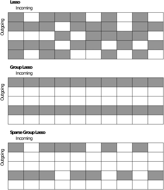
FIGURE 1. Comparison between lasso, group lasso, and sparse group lasso applied to a weight matrix. Entries in white are zero’ed out or removed; entries in gray remain.

2.2 Nonconvex Sparse Group Lasso

We recall that the ${\ell }_1$ norm is the tightest convex relaxation of the ${\ell }_0$ penalty, given by

${\left|\left|W_l\right|\right|}_0={\displaystyle \sum }_{g=1}^{N_l}{\displaystyle \sum }_{i=1}^{\#w_{l,g}}|w_{l,g,i}{|}_0(6)$

where

$|w{|}_0=\{\begin{array}{cc}1\text{ if }w\ne 0& \\ 0\text{ if }w=0& \end{array}$

when applied to the weight set $W_l$ of layer l. The ${\ell }_0$ penalty is non-convex and discontinuous. In addition, any ${\ell }_0$-regularized problem is NP-hard [23]. These properties make developing convergent and tractable algorithms for ${\ell }_0$-regularized problems difficult, thereby making ${\ell }_1$-regularized problems better alternatives to solve. However, the ${\ell }_0$-regularized problems have been shown to recover better solutions in terms of sparsity and/or accuracy than do ${\ell }_1$-regularized problems in various applications, such as compressed sensing [56], image restoration [8, 12, 19, 55, 102], MRI reconstruction [80], and machine learning [56, 94]. In particular, ${\ell }_0$-regularized inverse problems were demonstrated to be more robust against Poisson noise than are ${\ell }_1$-regualarized inverse problems [100].

A continuous alternative to the ${\ell }_0$ penalty is the SCAD penalty term [22, 58], given by

$\lambda {\left|\left|W_l\right|\right|}_{\text{SCAD}\left(a\right)}={\displaystyle \sum }_{g=1}^{N_l}{\displaystyle \sum }_{i=1}^{\#w_{l,g}}\lambda |w_{l,g,i}{|}_{\text{SCAD}\left(a\right)}(7)$

where

$\lambda |w{|}_{\text{SCAD}\left(a\right)}:=\{\begin{array}{cc}\lambda \left|w\right|& \text{ if }\left|w\right|<\lambda \\ \frac{2a\lambda \left|w\right|-w^2-{\lambda }^2}{2\left(a-1\right)}& \text{ if }\lambda \le \left|w\right|<a\lambda \\ \left(a+1\right){\lambda }^2/2& \text{ if }\left|w\right|\ge a\lambda \end{array}$

for $\lambda >0$ and $a>2$. This penalty term enjoys three properties – unbiasedness, sparsity, and continuity – while the ${\ell }_1$ norm, on the other hand, has only sparsity and continuity [22]. In linear and logistic regression, SCAD was shown to outperform ${\ell }_1$ in variable selection [22]. SCAD has been applied to wavelet approximation [5], bioinformatics [9, 84], and compressed sensing [64].

The transformed ${\ell }_1$ penalty term [68] also enjoys the properties of unbiasedness, sparsity, and continuity [58]. In fact, the regularizer is not just continuous but Lipschitz continuous [98]. The term is given by

${\left|\left|W_l\right|\right|}_{\text{TL}1\left(a\right)}={\displaystyle \sum }_{g=1}^{N_l}{\displaystyle \sum }_{i=1}^{\#w_{l,g}}|w_{l,g,i}{|}_{\text{TL}1\left(a\right)}(8)$

where

$|w{|}_{\text{TL}1\left(a\right)}=\frac{\left(a+1\right)\left|w\right|}{a+\left|w\right|}.$

In addition, it interpolates the ${\ell }_0$ and ${\ell }_1$ penalties through the parameter a [98] because

$\underset{a\to 0^{+}}{\text{lim}}\left|w{|}_{\text{TL}1\left(a\right)}=\right|w{|}_0\text{ and }\underset{a\to \infty }{\text{lim}}|w{|}_{\text{TL}1\left(a\right)}=\left|w\right|.$

The transformed ${\ell }_1$ penalty term was investigated and was shown to outperform ${\ell }_1$ in compressed sensing [79, 97, 98], deep learning [45, 61, 87], matrix completion [99], and epidemic forecasting [45].

Another Lipschitz continuous, nonconvex regularizer is the ${\ell }_1-\alpha {\ell }_2$ penalty given by

${\left|\left|W_l\right|\right|}_{{\ell }_1-\alpha {\ell }_2}={\left|\left|W_l\right|\right|}_1-\alpha {\left|\left|W_l\right|\right|}_2={\displaystyle \sum }_{g=1}^{N_l}{\displaystyle \sum }_{i=1}^{\#w_{l,g}}\left|w_{l,g,i}\right|-\alpha \sqrt{{\displaystyle \sum }_{g=1}^{N_l}{\displaystyle \sum }_{i=1}^{\#w_{l,g}}|w_{l,g,i}{|}^2},(9)$

where $\alpha \in \left(\mathrm{0,1}\right]$. In a series of works [50–52, 90], the penalty term ${\ell }_1-{\ell }_2$ with $\alpha =1$ yields better solutions than does ${\ell }_1$ in various compressed sensing applications especially when the sensing matrix is highly coherent or it violates the restricted isometry property condition. To guarantee exact recovery of sparse solution, ${\ell }_1-{\ell }_2$ only requires a relaxed variant of the null space property [79]. Furthermore, ${\ell }_1-\alpha {\ell }_2$ is more robust against impulsive noise in yielding sparse, accurate solutions for inverse problems than is ${\ell }_1$ [44]. Besides compressed sensing, it has been utilized in image denoising and deblurring [53], image segmentation [71], image inpainting [63], and hyperspectral demixing [21]. In deep learning application, the ${\ell }_1-{\ell }_2$ regularization was used to learn permutation matrices [59] for ShuffleNet [60, 101].

Due to the advantages and recent successes of the aforementioned nonconvex regularizers, we propose to replace the ${\ell }_1$ norm in Eq. 5 with nonconvex penalty terms. Hence, we propose a family of group regularizers called nonconvex sparse group lasso. The family includes the following:

${\mathrm{ℛ}}_{SG{L}_0}\left(W_l\right)={\mathrm{ℛ}}_{GL}\left(W_l\right)+{\left|\left|W_l\right|\right|}_0(10)$

${\mathrm{ℛ}}_{SGSCAD\left(a\right)}\left(W_l\right)={\mathrm{ℛ}}_{GL}\left(W_l\right)+{\left|\left|W_l\right|\right|}_{\text{SCAD}\left(a\right)}(11)$

${\mathrm{ℛ}}_{SGT{L}_1\left(a\right)}\left(W_l\right)={\mathrm{ℛ}}_{GL}\left(W_l\right)+{\left|\left|W_l\right|\right|}_{\text{TL}1\left(a\right)}(12)$

${\mathrm{ℛ}}_{SG{L}_1-\alpha L_2}\left(W_l\right)={\mathrm{ℛ}}_{GL}\left(W_l\right)+{\left|\left|W_l\right|\right|}_{{\ell }_1-\alpha {\ell }_2}.(13)$

Using these regularizers, we expect to obtain a sparser and/or more accurate network than from using the original sparse group lasso. The ${\ell }_1$ norm can also be replaced with other nonconvex penalties not mentioned in this paper. Refer to Refs. 3 and 85 to see other nonconvex penalties. However, we focus on the aforementioned nonconvex regularizers because they have closed-form proximal operators required by our proposed algorithm described in the next section.

2.3 Notations and Definitions

Before discussing the algorithm, we summarize notations that we will use to save space. They are the following:

If $V={\left\{V_l\right\}}_{l=1}^L$ and $W={\left\{W_l\right\}}_{l=1}^L$, then $\left(V,W\right):=\left({\left\{V_l\right\}}_{l=1}^L,{\left\{W_l\right\}}_{l=1}^L\right)=\left(V_1,\dots ,V_L,W_1,\dots ,W_L\right)$

$V^{+}:=V^{k+1}$

$\widetilde{\mathrm{ℒ}}\left(W\right):=\frac{1}{N}{{{\displaystyle \sum }}^{\text{}}}_{i=1}^N\mathrm{ℒ}\left(h\left(x_i,W\right),y_i\right)$

In addition, we define the proximal operator for the regularization function $r(\cdot )$ as follows:

${\text{prox}}_{\lambda r}\left(y\right)=\text{arg }\underset{x}{\text{min}}\lambda r\left(x\right)+\frac{1}{2}{\left|\left|x-y\right|\right|}_2^2$

for $\lambda >0$.

2.4 Numerical Optimization

We develop a general algorithm framework to solve

$\underset{W}{\text{min}}\widetilde{\mathrm{ℒ}}\left(W\right)+\lambda {\displaystyle \sum _{l=1}^L\mathrm{ℛ}\left(W_l\right)}=\widetilde{\mathrm{ℒ}}\left(W\right)+{\displaystyle \sum _{l=1}^L\left[\lambda {\mathrm{ℛ}}_{GL}\left(W_l\right)+\lambda r\left(W_l\right)\right]}(14)$

where $W={\left\{W_l\right\}}_{l=1}^L$, $\mathrm{ℛ}$ is either ${\mathrm{ℛ}}_{SG{L}_1}$ or one of the nonconvex regularizers Eqs. 10–13, and $r(\cdot )$ is the corresponding sparsity-inducing regularizer. Throughout the paper, our assumption on Eq. 14 is the following:

Assumption 1. The function $\widetilde{\mathrm{ℒ}}$ is continuously differentiable with respect to $W_l$ for each $l=1,\dots ,L$.

By introducing an auxiliary variable $V={\left\{V_l\right\}}_{l=1}^L$ for (14), we have a constrained optimization problem:

$\begin{array}{l}\underset{V,W}{\text{min}}\widetilde{\mathrm{ℒ}}\left(W\right)+\stackrel{L}{{\displaystyle \sum }_{l=1}}\left(\lambda {\mathrm{ℛ}}_{GL}\left(W_l\right)+\lambda r\left(V_l\right)\right)\\ \text{s}\text{.t}\text{. }{V}_l=W_{l}l=1,\dots ,L.\end{array}(15)$

The constraints can be relaxed by adding the quadratic penalty terms with $\beta >0$ so that we have

$\underset{V,W}{\text{min}}{F}_{\beta }\left(V,W\right):=\widetilde{\mathrm{ℒ}}\left(W\right)+{\displaystyle \sum }_{l=1}^L[\lambda {\mathrm{ℛ}}_{GL}\left(W_l\right)+\lambda r\left(V_l\right)+\frac{\beta }{2}{\left|\left|V_l-W_l\right|\right|}_2^2].(16)$

With β fixed, Eq. 16 can be solved by alternating minimization:

$W^{k+1}={\text{arg min}}_W{F}_{\beta }\left(V^k,W\right)(\mathrm{17a})$

$V^{k+1}={\text{arg min}}_V{F}_{\beta }\left(V,W^{k+1}\right).(\mathrm{17b})$

To solve Eq. 17a, we simultaneously update $W_l$ for $l=1,\dots L$ by gradient descent

$W_l^{k+1}=W_l^k-\gamma \left[{\nabla }_{W_l}\widetilde{\mathrm{ℒ}}\left(W^k\right)+\lambda {\partial }_{W_l}{\mathrm{ℛ}}_{GL}\left(W_l^k\right)-\beta \left(V_l^k-W_l^k\right)\right](18)$

where $\gamma >0$ is the learning rate and ${\partial }_{W_l}{\mathrm{ℛ}}_{GL}$ is the subdifferential of ${\mathrm{ℛ}}_{GL}$ with respect to $W_l$. In practice, Eq. 18 is performed using stochastic gradient descent (or one of its variants) with mini-batches due to the large-size computation dealing with the amount of data and weight parameters that a typical DNN has.

To update V, we see that Eq. 17b can be rewritten as

$V^{k+1}={\text{arg min}}_V{\displaystyle \sum }_{l=1}^L\left(\frac{\lambda }{\beta }r\left(V_l\right)+\frac{1}{2}{\left|\left|V_l-W_l\right|\right|}_2^2\right)=\left({\text{prox}}_{\frac{\lambda }{\beta }r}\left(W_1\right),\dots ,{\text{prox}}_{\frac{\lambda }{\beta }r}\left(W_L\right)\right).(19)$

The proximal operators for the considered regularizers are thresholding functions as their closed-form solutions, and as a result, the V update simplifies to thresholding W. The regularization functions and their corresponding proximal operators are summarized in Table 1.

TABLE 1

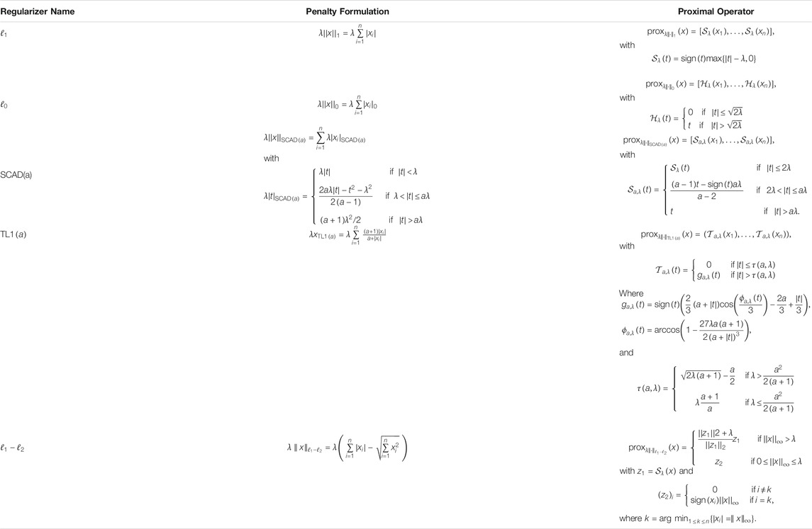
TABLE 1. Regularization penalties and their corresponding proximal operators with $\lambda >0$.

ALGORITHM 1:

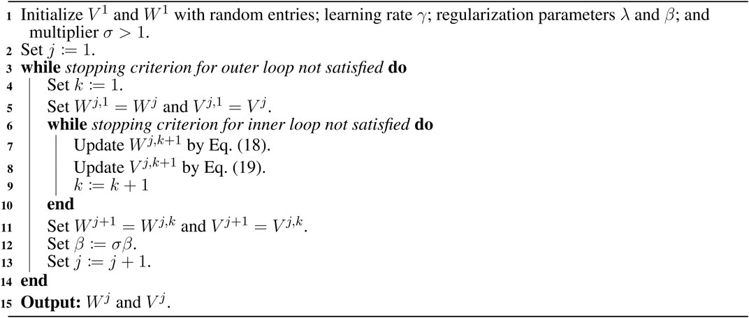
Algorithm 1:. Algorithm for Nonconvex Sparse Group Lasso RegularizationFAMS_fams-2020-529564_gs_fx1

Incorporating the algorithm that solves the quadratic penalty problem Eq. 16, we now develop a general algorithm to solve Eq. 14. We solve a sequence of quadratic penalty problems Eq. 16 with $\beta \in {\left\{{\beta }_j\right\}}_{j=1}^{\infty }$ where ${\beta }_j\uparrow \infty$. This will yield a sequence ${\left\{\left(V^j,W^j\right)\right\}}_{j=1}^{\infty }$ so that $W^j\to W^{\text{*}}$, a solution to (14). This algorithm is based on the quadratic penalty method [69] and the penalty decomposition method [56]. The algorithm is summarized in Algorithm 1.

An alternative algorithm to solve Eq. 14 is proximal gradient descent [70]. By this method, the update for $W_l,l=1,\dots ,L$, is

$W_l^{k+1}={\text{prox}}_{\gamma \lambda r}\left\{W_l^k-\gamma \left[{\nabla }_{W_l}\widetilde{\mathrm{ℒ}}\left(W^k\right)+\lambda {\partial }_{W_l}{\mathrm{ℛ}}_{GL}\left(W_l^k\right)\right]\right\}.(20)$

Using this algorithm results in weight parameters with some already zero’ed out.

However, the advantage of our proposed algorithm lies in Eq. 17a, written more specifically as

$W_l^{k+1}={\text{arg min}}_{W_l}\widetilde{\mathrm{ℒ}}\left(W\right)+{\mathrm{ℛ}}_{GL}\left(W_l\right)+\frac{\beta }{2}{\left|\left|V_l-W_l\right|\right|}_2^2(21)$

$={\text{arg min}}_{W_l}\widetilde{\mathrm{ℒ}}\left(W\right)+{\mathrm{ℛ}}_{GL}\left(W_l\right)+\frac{\beta }{2}\stackrel{\#W_l}{{\displaystyle \sum }_{i=1}}{\left(v_{l,i}-w_{l,i}\right)}^2.$

We see that this step performs exact weight decay or ${\ell }_2$ regularization on weights $w_{l,i}$ whenever $v_{l,i}=0$. On the other hand, when $v_{l,i}\ne 0$, the effect of ${\ell }_2$ regularization is mitigated on the corresponding weight $w_{l,i}$ based on the absolute difference $\left|v_{l,i}-w_{l,i}\right|$. Using ${\ell }_2$ regularization was shown to give superior pruning results in terms of accuracy by Han et al. [26]. Our proposed algorithm can be perceived as an adaptive ${\ell }_2$ regularization method, where Eq. 17b identifies which weights to perform exact ${\ell }_2$ regularization on and Eq. 17a updates and regularizes the weights accordingly.

2.5 Convergence Analysis

To establish convergence for the proposed algorithm, the results below state that the accumulation point of the sequence generated by Eqs 17a and 17b is a block-coordinate minimizer, and an accumulation point generated by Algorithm 1 is a sparse feasible solution to (15). Proofs are provided in Section 5. Unfortunately, the feasible solution generated may not be a local minimizer of Eq. 15 because the loss function $\mathrm{ℒ}\left(\cdot ,\cdot \right)$ is nonconvex. However, it was shown in [18] that a similar algorithm to Algorithm 1, but for fixed β in a bounded interval, generates an approximate global solution with high probability for a one-layer CNN with ReLu activation function.

Theorem 2. Let ${\left\{\left(V^k,W^k\right)\right\}}_{k=1}^{\infty }$ be a sequence generated by the alternating minimization algorithm Eqs. 17a and 17b, where $r(\cdot )$ is ${\ell }_0$, ${\ell }_1$, transformed ${\ell }_1$, ${\ell }_1-\alpha {\ell }_2$, or SCAD. If $\left(V^{\text{*}},W^{\text{*}}\right)$ is an accumulation point of ${\left\{\left(V^k,W^k\right)\right\}}_{k=1}^{\infty }$, then $\left(V^{\text{*}},W^{\text{*}}\right)$ is a block-coordinate minimizer of Eq. 16. that is

$V^{\text{*}}\in \text{arg }\underset{V}{\text{min}}{F}_{\beta }\left(V,W^{\text{*}}\right)$

$W^{\text{*}}\in \text{arg }\underset{W}{\text{min}}{F}_{\beta }\left(V^{\text{*}},W\right).$

Theorem 3. Let ${\left\{\left(V^k,W^k,{\beta }_k\right)\right\}}_{k=1}^{\infty }$ be a sequence generated by Algorithm 1. Suppose that ${\left\{F_{{\beta }_k}\left(V^k,W^k\right)\right\}}_{k=1}^{\infty }$ is uniformly bounded. If $(V^{\text{*}},W^{\text{*}})$ is an accumulation point of ${\left\{\left(V^k,W^k\right)\right\}}_{k=1}^{\infty }$, then $\left(V^{\text{*}},W^{\text{*}}\right)$ is a feasible solution to Eq. 15, that is $V^{\text{*}}=W^{\text{*}}$.

Remark: To safely ensure that ${\left\{F_{{\beta }_k}\left(V^k,W^k\right)\right\}}_{k=1}^{\infty }$ is uniformly bounded in practice, we can find a feasible solution $\left(V^{\text{feas}},W^{\text{feas}}\right)$ to (15) and impose a bound M such that

$M\ge \text{max}\left\{\tilde{L}\left(W^{\text{feas}}\right)+\lambda {\displaystyle \sum }_{l=1}^L\mathrm{ℛ}\left(W_l^{\text{feas}}\right),\underset{W}{\text{min}}{F}_{{\beta }_0}\left(V^1,W\right)\right\}.$

If ${\text{min}}_W{F}_{{\beta }_{k+1}}\left(V^k,W\right)>M$, then we set $V^{k+1}=W^{\text{feas}}$. This strategy is based on Ref. 56. However, in our numerical experiments, we have not yet encountered $F_{{\beta }_k}\left(V^k,W^k\right)$ to diverge.

3 Numerical Experiments

3.1 Application to Deep Neural Networks

We compare the proposed nonconvex sparse group lasso against four other methods as baselines: group lasso, sparse group lasso ($SG{L}_1$), CGES proposed in Ref. 92, and the group variant of ${\ell }_0$ regularization (denoted as ${\ell }_0$ for simplicity) proposed in Ref. 54. $SG{L}_1$ is optimized using the same algorithm proposed for nonconvex sparse group lasso. For the group terms, the weights are grouped together based on the filters or output channels, which we will refer to as neurons. We trained various CNN architectures on MNIST [41] and CIFAR 10/100 [38]. The MNIST dataset consists of 60k training images and 10k test images. MNIST is trained on two simple CNN architectures: LeNet-5-Caffe [31, 41] and a 4-layer CNN with two convolutional layers (32 and 64 channels, respectively) and an intermediate layer of 1000 fully connected neurons. CIFAR 10/100 is a dataset that has 10/100 classes split into 50k training images and 10k test images. It is trained on Resnets [28] and wide Resnets [95]. Throughout all of our experiments, for $SGSCAD\left(a\right)$, we set $a=3.7$ as suggested in [22]; for $SGT{L}_1\left(a\right)$, we set $a=1.0$ as suggested in Ref. 99; and for $SG{L}_1-L_2$, we set $\alpha =1.0$ as suggested by the literatures [50–52, 90]. For CGES, we have ${\mu }_l=l/L$. Because the optimization algorithms do not drive most, if not all, the weights and neurons to zeroes, we have to set them to zeroes when their values are below a certain threshold. In our experiments, if the absolute weights are below ${10}^{-5}$, we set them to zeroes. Then, weight sparsity is defined to be the percentage of zero weights with respect to the total number of weights trained in the network. If the normalized sum of the absolute values of the weights of the neuron is less than ${10}^{-5}$, then the weights of the neuron are set to zeroes. Neuron sparsity is defined to be the percentage of neurons whose weights are zeroes with respect to the total number of neurons in the network.

3.1.1 MNIST Classification

MNIST is trained on Lenet-5-Caffe, which has four layers with 1,370 total neurons and 431,080 total weight parameters. All layers of the network are applied with strictly the same type of regularization. No other regularization methods (e.g., dropout and batch normalization) are used. The network is optimized using Adam [37] with initial learning rate 0.001. For every 40 epochs, the learning rate decays by a factor of 0.1. We set the regularization parameter to the following values: $\lambda =\alpha /60000$ for $\alpha \in \left\{0.1,0.2,0.3,0.4,0.5\right\}$. For $SG{L}_1$ and nonconvex sparse group lasso, we set $\beta =25\alpha /60000$, and for every 40 epochs, β increases by a factor of $\sigma =1.25$. The network is trained for 200 epochs across 5 runs.

Table 2 reports the mean results for test error, weight sparsity, and neuron sparsity across five runs of Lenet-5-Caffe trained after 200 epochs. We see that although CGES has the lowest test errors at $\alpha \in \left\{0.1,0.3,0.4\right\}$ and the largest weight sparsity for all $\alpha \in \left\{0.1,0.2,\dots ,0.5\right\}$, nonconvex sparse group lasso’s test errors and weight sparsity are comparable. Additionally, nonconvex sparse group lasso’s neuron sparsity is nearly two times larger than the neuron sparsity attained by CGES. Across all parameters and methods, SGL₀ with $\alpha =0.5$ attains the best average test error of 0.630 with average weight sparsity 95.7% and neuron sparsity 80.7%. Furthermore, its test error is lower than the test errors of other nonconvex sparse group lasso regularization methods for all α’s tested. Generally, $SG{L}_1$ and nonconvex sparse group lasso outperform ${\ell }_0$ regularization proposed by Louizos et al. [54] and group lasso by average weight and neuron sparsity.

TABLE 2

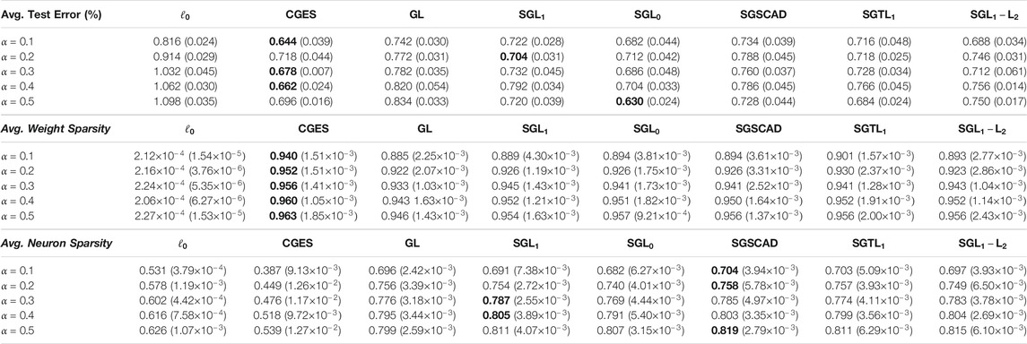
TABLE 2. Average test error, weight sparsity, and neuron sparsity of Lenet-5 models trained on MNIST after 200 epochs across 5 runs. Standard deviations are in parentheses.

Table 3 reports the mean results for test error, weight sparsity, and neuron sparsity of the Lenet-5-Caffe models with the lowest test errors from the five runs. According to the results, the best test errors are attained by $SG{L}_0$ at $\alpha =0.3,0.5$; $SG{L}_1-L_2$ at $\alpha =0.2$; and CGES at $\alpha =0.1,0.4$. For average weight sparsity, $SG{L}_0$ attains the largest weight sparsity at $\alpha \in \left\{0.2,0.3,0.4,0.5\right\}$. For average neuron sparsity, the largest values are attained by $SGT{L}_1$ at $\alpha =0.1,0.2$; by $SG{L}_1$ at $\alpha =0.3$; and by $SG{L}_0$ at $\alpha =0.4,0.5$. Although $SG{L}_0$ does not outperform all the other methods across the board, its results are still comparable to the best results. Overall, we see that nonconvex sparse group lasso outperforms ${\ell }_0$ in test error, weight sparsity, and neuron sparsity and group lasso in weight and neuron sparsity.

TABLE 3

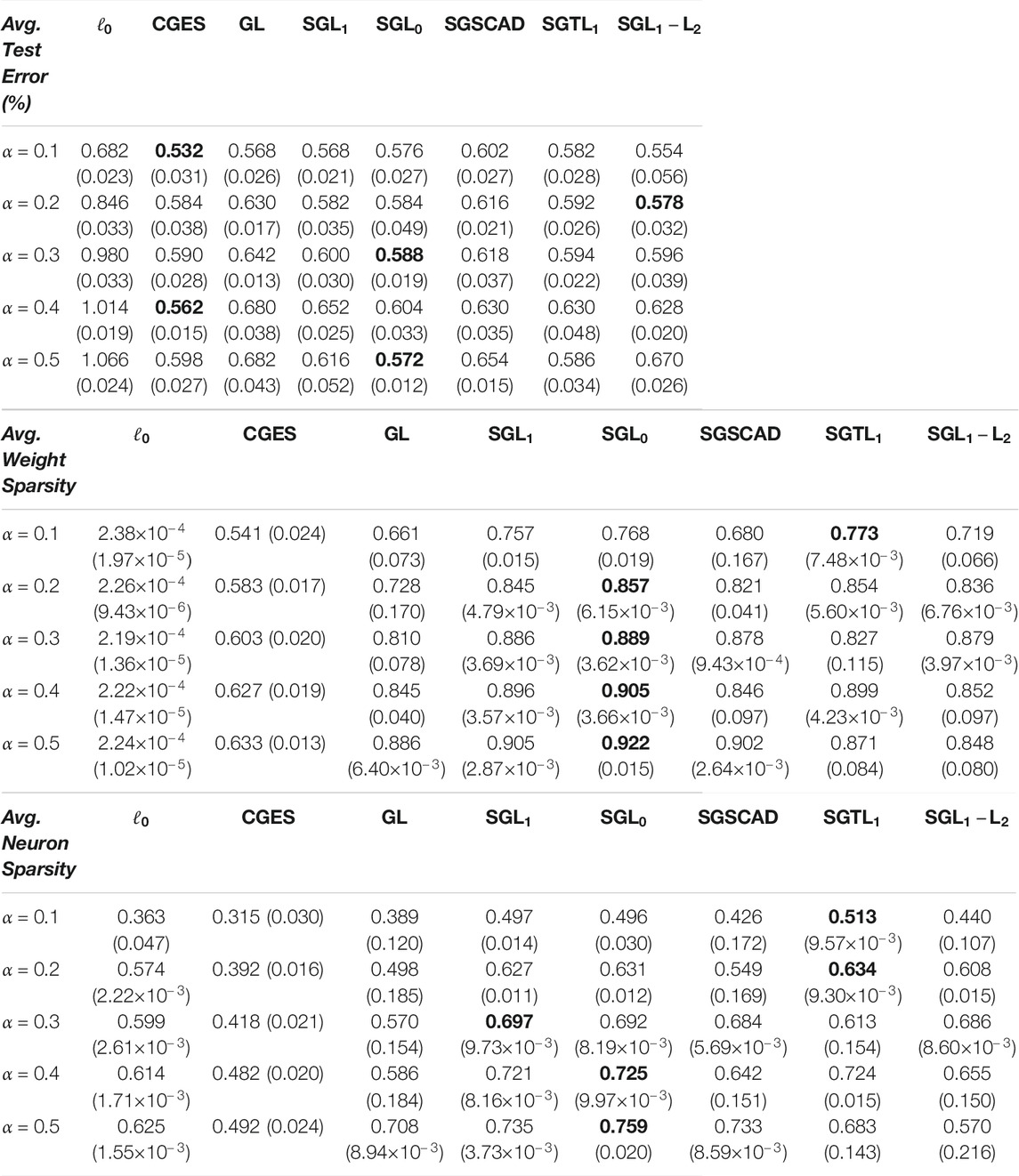
TABLE 3. Average test error, weight sparsity, and neuron sparsity of Lenet-5 models trained on MNIST with lowest test errors across 5 runs. Standard deviations are in parentheses.

MNIST is also trained on a 4-layer CNN with two convolutional layers with 32 and 64 channels, respectively, and an intermediate layer with 1000 neurons. Each convolutional layer has a $5\times 5$ convolutional filters. The 4-layer CNN has 2,120 total neurons and 1,087,010 total weight parameters. All layers of the network are applied with strictly the same type of regularization. The network is optimized with the same settings as Lenet-5-Caffe. However, the regularization parameter is different: we have $\lambda =\alpha /60000$ for $\alpha \in \left\{0.2,0.4,0.6,0.8,1.0\right\}$. For $SG{L}_1$ and nonconvex sparse group lasso, we set $\beta =5\alpha /60000$ and for every 40 epochs, β increases by a factor of $\sigma =1.25$. The network is trained for 200 epochs across 5 runs.

Table 4 reports the mean results for test error, weight sparsity, and neuron sparsity across five runs of the 4-layer CNN models trained after 200 epochs. Although CGES consistently has the highest weight sparsity, it does not yield the most accurate models until when $\alpha \ge 0.8$. Moreover, its neuron sparsity is smaller than the neuron sparsity by group lasso, $SG{L}_1$, and nonconvex group lasso when $\alpha \ge 0.6$. ${\ell }_0$ has the highest neuron sparsity for all α’s given, but its test errors are much greater. When $\alpha \le 0.6$, $SGSCAD$ yields the most accurate models at $\alpha =0.2,0.6$ while $SG{L}_1$ yields one at $\alpha =0.4$. Overall, we see that nonconvex group lasso has comparable weight sparsity and neuron sparsity as group lasso and $SG{L}_1$.

TABLE 4

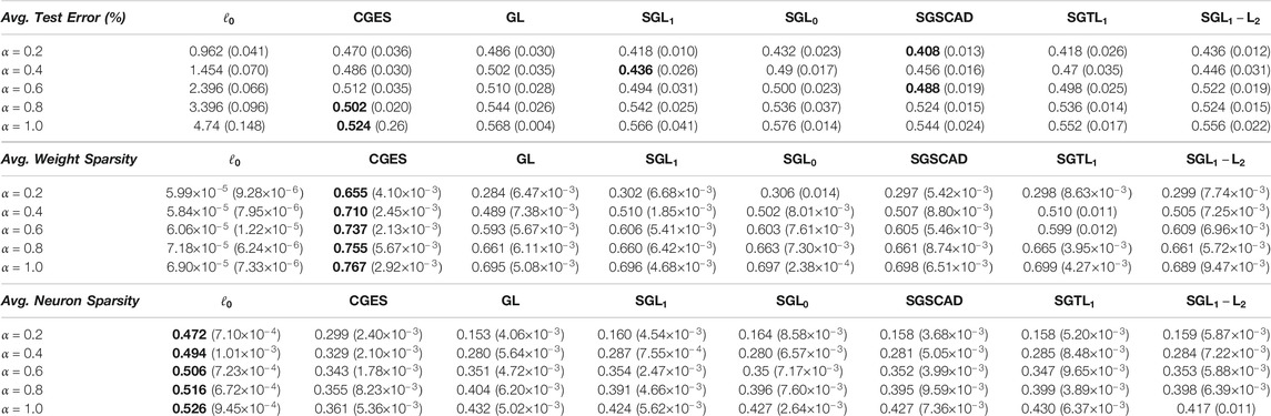
TABLE 4. Average test error, weight sparsity, and neuron sparsity of 4-layer CNN models trained on MNIST after 200 epochs across 5 runs. Standard deviations are in parentheses.

Table 5 reports the mean results for test error, weight sparsity, and neuron sparsity of the 4-layer CNN models with the lowest test errors from the five runs. At $\alpha =0.2$, $SG{L}_1$ and $SGSCAD$ have the lowest test errors, but their weight sparsity are exceeded by CGES and their neuron sparsity are exceeded by ${\ell }_0$. At $\alpha =0.4$, $SG{L}_1-L_2$ has the lowest test error, but its weight sparsity and neuron sparsity are exceeded by CGES and ${\ell }_0$, respectively. At $\alpha =0.6$, $SG{L}_1$ has the lowest test error, but $SGSCAD$ has the largest weight sparsity with comparable test error. At $\alpha \ge 0.8$, CGES has the lowest test error, but its weight sparsity is exceeded by group lasso, $SG{L}_1$, and the nonconvex group lasso regularizers, which all have slightly higher test error. At $\alpha =0.8$, the neuron sparsity of CGES is comparable to the neuron sparsity of group lasso, $SG{L}_1$, and the nonconvex group lasso regularizers. At $\alpha =1.0$, group lasso has the highest neuron sparsity, but nonconvex group lasso has slightly lower neuron sparsity. In general, weight sparsity of nonconvex group lasso is comparable to or larger than the weight sparsity of group lasso and $SG{L}_1$.

TABLE 5

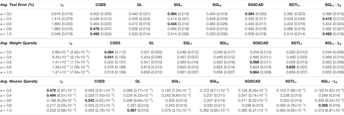
TABLE 5. Average test error, weight sparsity, and neuron sparsity of 4-layer CNN models trained on MNIST with lowest test errors across 5 runs. Standard deviations are in parentheses.

3.1.2 CIFAR Classification

CIFAR 10/100 is trained on Resnet-40 and wide Resnet with depth 28 and width 10 (WRN-28-10). Resnet-40 has approximately 570,000 weight parameters and 1520 neurons while WRN-28-10 has approximately 36,500,000 weight parameters and 10,736 neurons. The networks are optimized using stochastic gradient descent with initial learning rate 0.1. After every 60 epochs, learning rate decays by a factor of 0.2. Strictly the same type of regularization is applied to the weights of the hidden layer where dropout is utilized in the residual block. We vary the regularization parameter $\lambda =\alpha /50000$. For Resnet-40, we have $\alpha \in \left\{1.0,1.5,2.0,2.5,3.0\right\}$ for CIFAR 10 and $\alpha \in \left\{2.0,2.5,3.0,3.5,4.0\right\}$ for CIFAR 100. For $SG{L}_1$ and nonconvex sparse group lasso, we set $\beta =15\alpha /50000$ for Resnet-40 and $\beta =25\alpha /50000$ for WRN-28-10. For every 20 epochs, β increases by a factor of $\sigma =1.25$. The networks are trained for 200 epochs across 5 runs. We excluded ${\ell }_0$ regularization by Louizos et al. [54] because it was unstable for the provided α’s. Furthermore, we only analyze the models with the lowest test errors since the test errors did not stabilize by the end of the 200 epochs in our experiments.

Table 6 reports mean test error, weight sparsity, and neuron sparsity across the Resnet-40 models trained on CIFAR 10 with the lowest test errors from the five runs. Group lasso has the lowest test errors for all α’s provided while CGES, $SG{L}_1$, and nonconvex sparse group lasso are higher by at most 1.1%. When $\alpha \le 1.5$, CGES has the largest weight sparsity while $SGSCAD$, $SGT{L}_1$$SG{L}_1-SG{L}_2$ have larger weight sparsity than does group lasso. At $\alpha =2.0,2.5$, $SGSCAD$ has the largest weight sparsity. At $\alpha =3.0$, $SG{L}_1$ has the largest weight sparsity with comparable test error as the nonconvex group lasso regularizers. For neuron sparsity, $SG{L}_1-L_2$ has the largest at $\alpha =1.0$ while $SGSCAD$ has the largest at $\alpha =1.5,2.0$. However, at $\alpha =2.5,3.0$, group lasso has the largest neuron sparsity. For all α’s tested, $SGSCAD$ has higher weight sparsity and neuron sparsity than does $SG{L}_1$ but with comparable test error.

TABLE 6

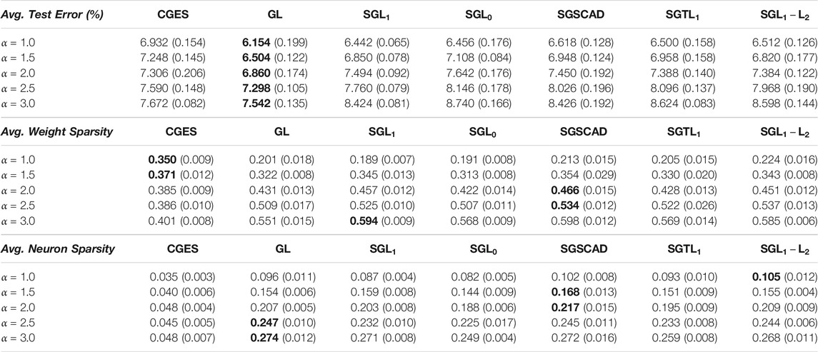
TABLE 6. Average test error, weight sparsity, and neuron sparsity of Resnet-40 models trained on CIFAR 10 with lowest test errors across 5 runs. Standard deviations are in parentheses.

Table 7 reports mean test error, weight sparsity, and neuron sparsity across the Resnet-40 models trained on CIFAR 100 with the lowest test errors from the five runs. Group lasso has the lowest test errors for $\alpha \le 3.5$ while CGES has the lowest test error at $\alpha =4.0$. However, the weight sparsity and the neuron sparsity of group lasso are lower than the sparsity of $SG{L}_1$ and some of the nonconvex sparse group lasso regularizers. CGES has the lowest neuron sparsity across all α’s. Among the nonconvex group lasso penalties, $SGSCAD$ has the best test errors, which are lower than the test errors of $SG{L}_1$ for all α’s except 2.5.

TABLE 7

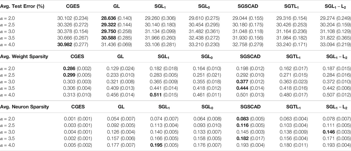
TABLE 7. Average test error, weight sparsity, and neuron sparsity of Resnet-40 models trained on CIFAR 100 with lowest test errors across 5 runs. Standard deviations are in parentheses.

Table 8 reports mean test error, weight sparsity, and neuron sparsity across the WRN-28-10 models trained on CIFAR 10 with the lowest test errors from the five runs. The best test errors are attained by $SGT{L}_1$ at $\alpha =0.05,0.2,0.5$; by CGES at $\alpha =0.01$; and by $SG{L}_1$ at $\alpha =0.1$. Weight sparsity of CGES outperforms the other methods only when $\alpha =0.01,0.05,0.1$, but it underperforms when $\alpha \ge 0.2$. Weight sparsity levels between group lasso and nonconvex group lasso are comparable across all α. For neuron sparsity, $SG{L}_1-L_2$ attains the largest values at $\alpha =0.02,0.1,0.2$. Nevertheless, the other nonconvex sparse group lasso methods have comparable neuron sparsity. Overall, $SG{L}_1$, $SG{L}_0$, $SGSCAD$, and $SGT{L}_1$ outperform group lasso in test error while having similar or higher weight and neuron sparsity.

TABLE 8

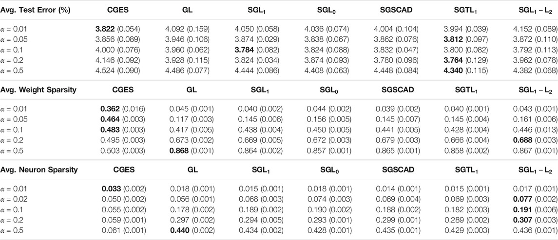
TABLE 8. Average test error, weight sparsity, and neuron sparsity of WRN-28-10 models trained on CIFAR 10 with lowest test errors across 5 runs. Standard deviations are in parentheses.

Table 9 reports mean test error, weight sparsity, and neuron sparsity across the WRN-28-10 models trained on CIFAR 100 with the lowest test errors from the five runs. According to the results, the best test errors are attained by CGES when $\alpha =0.01,0.05$; by $SGSCAD$ when $\alpha =0.1,0.5$; and by $SGT{L}_1$ when $\alpha =0.2$. Although CGES has the largest weight sparsity for $\alpha =0.01,0.05,0.1,0.2$, we see that its test error increases as α increases. When $\alpha =0.5$, the best weight sparsity is attained by $SGSCAD$, but the other methods have comparable weight sparsity. The best neuron sparsity is attained by CGES at $\alpha =0.01,0.02$; by $SG{L}_1-L_2$ at $\alpha =0.1,0.2$; and by $SGSCAD$ at $\alpha =0.5$. The neuron sparsity among the nonconvex sparse group lasso methods are comparable. For $\alpha \le 0.2$, we see that $SG{L}_1$ and nonconvex sparse group lasso outperform group lasso in test error across α while having comparable weight and neuron sparsity.

TABLE 9

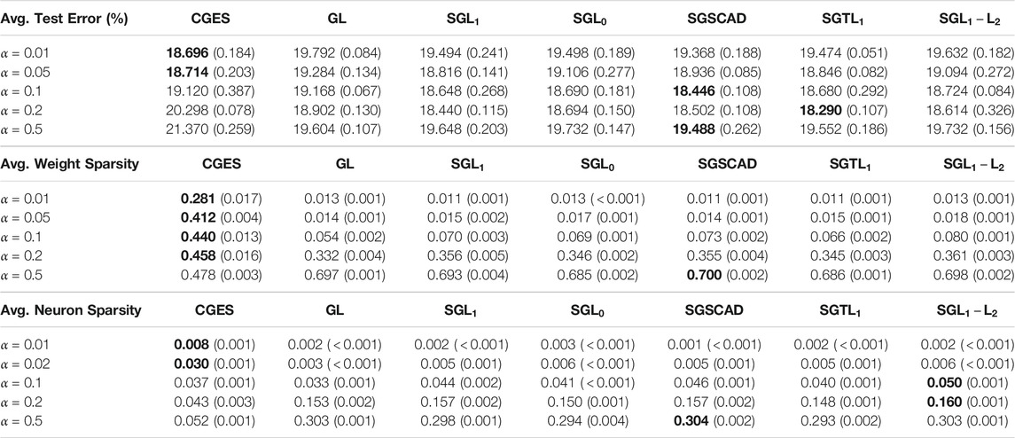
TABLE 9. Average test error, weight sparsity, and neuron sparsity of WRN-28-10 models trained on CIFAR 100 with lowest test errors across 5 runs. Standard deviations are in parentheses.

3.2 Algorithm Comparison

We compare the proposed Algorithm 1 with direct stochastic gradient descent, where the gradient of the regularizer is approximated by backpropagation, and proximal gradient descent, discussed in Section 2.4, by applying them to $SG{L}_1$ on Lenet-5 trained on MNIST. The parameter setting for this CNN is discussed in Section 3.1.1. Table 10 reports the mean results for test error, weight sparsity, and neuron sparsity across five models trained after 200 epochs while Figure 2 provides visualizations. Table 11 and Figure 3 record mean statistics for models with the lowest test errors from the five runs. According to the results, proximal stochastic gradient descent attains the highest level of weight sparsity and neuron sparsity for models trained after 200 epochs and models with the lowest test error. However, their test errors are the highest among the three algorithms. On the other hand, our proposed algorithm attains the lowest test errors. For models trained after 200 epochs, the weight sparsity and neuron sparsity attained by Algorithm 1 are comparable to the sparsity attained by direct stochastic gradient descent. For models with the lowest test errors generated from their respective runs, the weight sparsity and neuron sparsity by the proposed algorithm are better than the sparsity by direct stochastic gradient descent. Therefore, our proposed algorithm generates the most accurate model with satisfactory sparsity among the three algorithms for sparse regularization.

TABLE 10

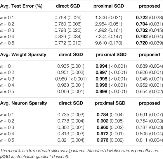
TABLE 10. Average test error, weight sparsity, and neuron sparsity of ${\text{SGL}}_1$-regularized Lenet-5 models trained on MNIST after 200 epochs across 5 runs.

FIGURE 2

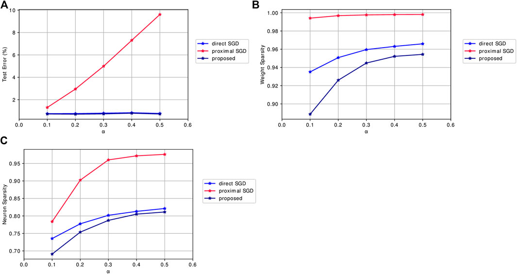
FIGURE 2. Mean results of algorithms applied to SGL₁ for Lenet-5 models trained on MNIST for 200 epochs across 5 runs when varying the regularization parameter $\lambda =\alpha /60000$ when $\alpha \in \left\{0.1,0.2,0.3,0.4,0.5\right\}$. (A) Mean test error. (B) Mean weight sparsity. (C) Mean neuron sparsity.

TABLE 11

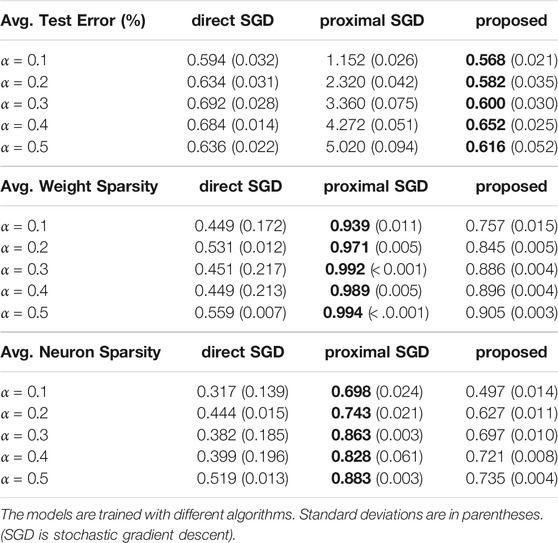
TABLE 11. Average test error, weight sparsity, and neuron sparsity of ${\text{SGL}}_1$-regularized Lenet-5 models trained on MNIST with lowest test errors across 5 runs.

FIGURE 3

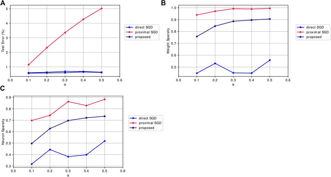
FIGURE 3. Mean results of algorithms applied to SGL₁ for Lenet-5 models trained on MNIST with lowest test errors across 5 runs when varying the regularization parameter $\lambda =\alpha /60000$ when $\alpha \in \left\{0.1,0.2,0.3,0.4,0.5\right\}$. (A) Mean test error. (B) Mean weight sparsity. (C) Mean neuron sparsity.

4 Conclusion and Future Work

In this work, we propose nonconvex sparse group lasso, a nonconvex extension of sparse group lasso. The ${\ell }_1$ norm in sparse group lasso on the weight parameters is replaced with a nonconvex regularizer whose proximal operator is a thresholding function. Taking advantage of this property, we develop a new algorithm to optimize loss functions regularized with nonconvex sparse group lasso for CNNs in order to attain a sparse network with competitive accuracy. We compare the proposed family of regularizers with various baseline methods on MNIST and CIFAR 10/100 on different CNNs. The experimental results demonstrate that in general, nonconvex sparse group lasso generates a more accurate and/or more compressed CNN than does group lasso. In addition, we compare our proposed algorithm to direct stochastic gradient descent and proximal gradient descent on Lenet-5 trained on MNIST. The results show that the proposed algorithm to solve $SG{L}_1$ yields a satisfactorily sparse network with lower test error than do the other two algorithms.

According to the numerical results, there is no single sparse regularizer that outperforms all other on any CNN trained on a given dataset. One regularizer may perform well in one case while it may perform worse on a different case. Due to the myriad of sparse regularizers to select from and the various parameters to tune, especially for one CNN trained on a given dataset, one direction is to develop an automatic machine learning framework that efficiently selects the right regularizer and parameters. In recent works, automatic machine learning can be represented as a matrix completion problem [88] and a statistical learning problem [24]. These frameworks can be adapted for selecting the best sparse regularizer, thus saving time for users who are training sparse CNNs.

5 Proofs

We provide proofs for the results discussed in Section 2.5.

5.1 Proof of Theorem 2

By Eqs 17a and 17b, for each $k\in \mathrm{\mathbb{N}}$, we have

$F_{\beta }\left(V^k,W^{k+1}\right)\le F_{\beta }\left(V^k,W\right)(22)$

for all W, and

$F_{\beta }\left(V^{k+1},W^{k+1}\right)\le F_{\beta }\left(V,W^{k+1}\right)(23)$

for all V. By Eq. 23, we have

$F_{\beta }\left(V^{+},W^{+}\right)\le F_{\beta }\left(V^k,W^{+}\right)(24)$

for each $k\in \mathrm{\mathbb{N}}$. Altogether, we have

$F_{\beta }\left(V^{+},W^{+}\right)\le F_{\beta }\left(V^k,W^k\right)(25)$

for each $k\in \mathrm{\mathbb{N}}$, so ${\left\{F_{\beta }\left(V^k,W^k\right)\right\}}_{k=1}^{\infty }$ is nonincreasing. Since $F_{\beta }\left(V^k,W^k\right)\ge 0$ for all $k\in \mathrm{\mathbb{N}}$, its limit $\underset{k\to \infty }{\text{lim}}{F}_{\beta }\left(V^k,W^k\right)$ exists. From Eqs. 22–24, we have

$F_{\beta }\left(V^{+},W^{+}\right)\le F_{\beta }\left(V^k,W^{+}\right)\le F_{\beta }\left(V^k,W^k\right).$

Taking the limit gives us

$\underset{k\to \infty }{\text{lim}}{F}_{\beta }\left(V^k,W^{+}\right)=\underset{k\to \infty }{\text{lim}}{F}_{\beta }\left(V^k,W^k\right).(26)$

Since $\left(V^{\text{*}},W^{\text{*}}\right)$ is an accumulation point of ${\left\{\left(V^k,W^k\right)\right\}}_{k=1}^{\infty }$, there exists a subsequence K such that

$\underset{k\in K\to \infty }{\text{lim}}\left(V^k,W^k\right)=\left(V^{\text{*}},W^{\text{*}}\right).(27)$

Because $r(\cdot )$ is lower semicontinuous and $\underset{k\in K\to \infty }{\text{lim}}{V}^k=V^{\text{*}}$, there exists $k^{\prime }\in K$ such that $k\ge k^{\prime }$ implies $r\left(V_l^k\right)\ge r\left(V_l^{\text{*}}\right)$ for each $l=1,\dots ,L$. Using this result along with Eq. 23, we obtain

$\begin{array}{c}{F}_{\beta }\left(V,W^k\right)\ge F_{\beta }\left(V^k,W^k\right)\\ =\widetilde{\mathrm{ℒ}}\left(W^k\right)+\stackrel{L}{{\displaystyle \sum }_{l=1}}\left[\lambda \left({\mathrm{ℛ}}_{GL}\left(W_l^k\right)+r\left(V_l^k\right)\right)+\frac{\beta }{2}{\left|\left|V_l^k-W_l^k\right|\right|}_2^2\right]\\ \ge \widetilde{\mathrm{ℒ}}\left(W^k\right)+\stackrel{L}{{\displaystyle \sum }_{l=1}}\left[\lambda \left({\mathrm{ℛ}}_{GL}\left(W_l^k\right)+r\left(V_l^{\text{*}}\right)\right)+\frac{\beta }{2}{\left|\left|V_l^k-W_l^k\right|\right|}_2^2\right]\end{array}$

for $k\ge k^{\prime }$. As $k\in K\to \infty$, we have

$F_{\beta }\left(V,W^{\text{*}}\right)\ge \widetilde{\mathrm{ℒ}}\left(W^{\text{*}}\right)+{\displaystyle \sum }_{l=1}^L\left[\lambda \left({\mathrm{ℛ}}_{GL}\left(W_l^{\text{*}}\right)+r\left(V_l^{\text{*}}\right)\right)+\frac{\beta }{2}{\left|\left|V_l^{\text{*}}-W_l^{\text{*}}\right|\right|}_2^2\right]=F_{\beta }\left(V^{\text{*}},W^{\text{*}}\right)(28)$

by continuity, so it follows that $V^{\text{*}}\in {\text{arg min}}_V{F}_{\beta }\left(V,W^{\text{*}}\right)$.

For notational convenience, let

${\widetilde{\mathrm{ℛ}}}_{\lambda ,\beta }\left(V,W\right):={\displaystyle \sum }_{l=1}^L\left[\lambda {\mathrm{ℛ}}_{GL}\left(W_l\right)+\frac{\beta }{2}{\left|\left|V_l-W_l\right|\right|}_2^2\right].(29)$

By Eq. 22, we have

$\begin{array}{c}\widetilde{\mathrm{ℒ}}\left(W\right)+{\widetilde{\mathrm{ℛ}}}_{\lambda ,\beta }\left(V^k,W\right)=F_{\beta }\left(V^k,W\right)-\lambda \stackrel{L}{{\displaystyle \sum }_{i=1}}r\left(V_l^k\right)\\ \ge F_{\beta }\left(V^k,W^{+}\right)-\lambda \stackrel{L}{{\displaystyle \sum }_{i=1}}r\left(V_l^k\right)=\widetilde{\mathrm{ℒ}}\left(W^{+}\right)+{\widetilde{\mathrm{ℛ}}}_{\lambda ,\beta }\left(V^k,W^{+}\right).\end{array}(30)$

Because $\underset{k\in K\to \infty }{\text{lim}}{V}^k$ exists, the sequence ${\left\{V^k\right\}}_{k\in K}$ is bounded. If $r(\cdot )$ is ${\ell }_0$, transformed ${\ell }_1$, or SCAD, then ${\left\{r\left(V^k\right)\right\}}_{k\in K}$ is bounded. If $r(\cdot )$ is ${\ell }_1$, then $r(\cdot )$ is coercive. If $r(\cdot )$ is ${\ell }_1-\alpha {\ell }_2$, then $r(\cdot )$ is bounded above by ${\ell }_1$. Overall, this follows that ${\left\{r\left(V^k\right)\right\}}_{k\in K}$ bounded as well. Hence, there exists a further subsequence $\overline{K}\subset K$ such that $\underset{k\in \overline{K}\to \infty }{\text{lim}}r\left(V^k\right)$ exists. So, we obtain

$\begin{array}{c}\underset{k\in \overline{K}\to \infty }{\text{lim}}\widetilde{\mathrm{ℒ}}\left(W^{+}\right)+{\widetilde{\mathrm{ℛ}}}_{\lambda ,\beta }\left(V^k,W^{+}\right)=\underset{k\in \overline{K}\to \infty }{\text{lim}}{F}_{\beta }\left(V^k,W^{+}\right)-\lambda \stackrel{L}{{\displaystyle \sum }_{i=1}}r\left(V_l^k\right)\\ =\underset{k\in \overline{K}\to \infty }{\text{lim}}{F}_{\beta }\left(V^k,W^{+}\right)-\underset{k\in \overline{K}\to \infty }{\text{lim}}\lambda \stackrel{L}{{\displaystyle \sum }_{i=1}}r\left(V_l^k\right)\\ =\underset{k\in \overline{K}\to \infty }{\text{lim}}{F}_{\beta }\left(V^k,W^k\right)-\underset{k\in \overline{K}\to \infty }{\text{lim}}\lambda \stackrel{L}{{\displaystyle \sum }_{i=1}}r\left(V_l^k\right)\\ =\underset{k\in \overline{K}\to \infty }{\text{lim}}{F}_{\beta }\left(V^k,W^k\right)-\lambda \stackrel{L}{{\displaystyle \sum }_{i=1}}r\left(V_l^k\right)\\ =\underset{k\in \overline{K}\to \mathrm{\infty }}{\text{lim}}\widetilde{\mathrm{ℒ}}\left(W^k\right)+{\widetilde{\mathrm{ℛ}}}_{\lambda ,\beta }\left(V^k,W^k\right)\\ =\widetilde{\mathrm{ℒ}}\left(W^{\text{*}}\right)+{\widetilde{\mathrm{ℛ}}}_{\lambda ,\beta }\left(W^{\text{*}},V^{\text{*}}\right)\end{array}(31)$

after applying Eq. 26 in the third inequality and by continuity in the last equality.

Taking the limit over the subsequence $\overline{K}$ in Eq. 30 and applying Eq. 31, we obtain

$\widetilde{\mathrm{ℒ}}\left(W\right)+{\widetilde{\mathrm{ℛ}}}_{\lambda ,\beta }\left(V^{\text{*}},W\right)\ge \widetilde{\mathrm{ℒ}}\left(W^{\text{*}}\right)+{\widetilde{\mathrm{ℛ}}}_{\lambda ,\beta }\left(W^{\text{*}},V^{\text{*}}\right)(32)$

by continuity. Adding ${{{\displaystyle \sum }}^{\text{}}}_{l=1}^{L}r\left(V_l^{\text{*}}\right)$ on both sides yields

$F_{\beta }\left(V^{\text{*}},W\right)\ge F_{\beta }\left(V^{\text{*}},W^{\text{*}}\right),(33)$

which follows that $W^{\text{*}}\in {\text{arg min}}_W{F}_{\beta }\left(V^{\text{*}},W\right)$. This completes the proof.

5.2 Proof of Theorem 3

Because $\left(V^{\text{*}},W^{\text{*}}\right)$ is an accumulation point, there exists a subsequence K such that $\underset{k\in K\to \infty }{\text{lim}}\left(V^k,W^k\right)=\left(V^{\text{*}},W^{\text{*}}\right)$. If ${\left\{F_{{\beta }_k}\left(V^k,W^k\right)\right\}}_{k=1}^{\infty }$ is uniformly bounded, there exists M such that $F_{{\beta }_k}\left(V^k,W^k\right)\le M$ for all $k\in \mathrm{\mathbb{N}}$. Then we have

$M\ge F_{{\beta }_k}\left(V^k,W^k\right)=\widetilde{\mathrm{ℒ}}\left(W\right)+{\displaystyle \sum }_{l=1}^L\left[\lambda {\mathrm{ℛ}}_{GL}\left(W_l\right)+\lambda r\left(V_l\right)+\frac{{\beta }_k}{2}{\left|\left|V_l-W_l\right|\right|}_2^2\right]\ge \frac{{\beta }_k}{2}{\displaystyle \sum }_{l=1}^L{\left|\left|V_l-W_l\right|\right|}_2^2$

As a result,

${\displaystyle \sum }_{l=1}^L{\left|\left|V_l^k-W_l^k\right|\right|}_2^2\le \frac{2}{{\beta }_k}M.(34)$

Taking the limit over $k\in K$, we have

${\displaystyle \sum }_{l=1}^L{\left|\left|V_l^{\text{*}}-W_l^{\text{*}}\right|\right|}_2^2=0,$

which follows that $V^{\text{*}}=W^{\text{*}}$. As a result, $\left(V^{\text{*}},W^{\text{*}}\right)$ is a feasible solution to Eq. 15.

Data Availability Statement

The datasets MNIST and CIFAR 10/100 for this study are available through the Pytorch package in Python. Codes for the numerical experiments in Section 3 are available at https://github.com/kbui1993/Official_Nonconvex_SGL.

Author Contributions

KB and FP performed the experiments and analysis. All authors contributed to the design, evaluation, discussions and production of the manuscript.

Funding

The work was partially supported by NSF grants IIS-1632935, DMS-1854434, DMS-1924548, DMS-1952644 and the Qualcomm Faculty Award.

Conflict of Interest

The authors declare that the research was conducted in the absence of any commercial or financial relationships that could be construed as a potential conflict of interest.

Acknowledgments

The authors would like to thank Thu Dinh for helpful conversations. They also thank Christos Louizos for answering our questions we had regarding his work in [54]. Lastly, the authors thank AWS Cloud Credits for Research and Google Cloud Platform (GCP) for providing cloud based computational resources for this work.

References

1. Aghasi, A, Abdi, A, Nguyen, N, and Romberg, J. Net-trim: convex pruning of deep neural networks with performance guarantee. In: Advances in Neural Information Processing Systems; 2017 Nov 23; Long Beach, CA. Pasadena, CA: NeurIPS (2017). p. 3177–86. doi:10.5555/3294996.3295077

PubMed Abstract | CrossRef Full Text | Google Scholar

2. Aghasi, A, Abdi, A, and Romberg, J. Fast convex pruning of deep neural networks. SIAM J Math Data Sci (2020). 2:158–188. doi:10.1137/19m1246468

PubMed Abstract | CrossRef Full Text | Google Scholar

3. Ahn, M, Pang, J-S, and Xin, J. Difference-of-convex learning: directional stationarity, optimality, and sparsity. SIAM J Optim. (2017). 27:1637–1665. doi:10.1137/16m1084754

PubMed Abstract | CrossRef Full Text | Google Scholar

4. Alvarez, JM, and Salzmann, M. Learning the number of neurons in deep networks In: Advances in Neural Information Processing Systems; 2018 Oct 11; Barcelona, Spain. Pasadena, CA: NeurIPS (2016). p. 2270–8.

Google Scholar

5. Antoniadis, A, and Fan, J. Regularization of wavelet approximations. J Am Stat Assoc. (2001). 96:939–67. doi:10.1198/016214501753208942

PubMed Abstract | CrossRef Full Text | Google Scholar

6. Ba, J, and Caruana, R. Do deep nets really need to be deep? Adv Neural Inf Process Syst. (2014). 2:2654–62. doi:10.5555/2969033.2969123

PubMed Abstract | CrossRef Full Text | Google Scholar

7. Bach, FR. Consistency of the group lasso and multiple kernel learning. J Mach Learn Res. (2008). 9:1179–225. doi:10.5555/1390681.1390721

PubMed Abstract | CrossRef Full Text | Google Scholar

8. Bao, C, Dong, B, Hou, L, Shen, Z, Zhang, X, and Zhang, X. Image restoration by minimizing zero norm of wavelet frame coefficients. Inverse Problems. (2016). 32:115004. doi:10.1088/0266-5611/32/11/115004

PubMed Abstract | CrossRef Full Text | Google Scholar

9. Breheny, P, and Huang, J. Coordinate descent algorithms for nonconvex penalized regression, with applications to biological feature selection. Ann Appl Stat. (2011). 5:232. doi:10.1214/10-aoas388

PubMed Abstract | CrossRef Full Text | Google Scholar

10. Candès, EJ, Li, X, Ma, Y, and Wright, J. Robust principal component analysis? J ACM. (2011). 58:1–37. doi:10.1145/1970392.1970395

PubMed Abstract | CrossRef Full Text | Google Scholar

11. Candès, EJ, Romberg, JK, and Tao, T. Stable signal recovery from incomplete and inaccurate measurements. Commun Pure Appl Math. (2006). 59:1207–23. doi:10.1002/cpa.20124

PubMed Abstract | CrossRef Full Text | Google Scholar

12. Chan, RH, Chan, TF, Shen, L, and Shen, Z. Wavelet algorithms for high-resolution image reconstruction. SIAM J Sci Comput. (2003). 24:1408–32. doi:10.1137/s1064827500383123

PubMed Abstract | CrossRef Full Text | Google Scholar

13. Chen, LC, Papandreou, G, Kokkinos, I, Murphy, K, and Yuille, AL (2018). Deeplab: Semantic image segmentation with deep convolutional nets, atrous convolution, and fully connected crfs. IEEE Trans Pattern Anal Mach Intell. 40, 834–848doi:10.1109/TPAMI.2017.2699184

PubMed Abstract | CrossRef Full Text | Google Scholar

14. Cheng, Y, Wang, D, Zhou, P, and Zhang, T. A survey of model compression and acceleration for deep neural networks. Preprint repository name [Preprint] (2017). Available from: https://arxiv.org/abs/1710.09282.

Google Scholar

15. Cheng, Y, Wang, D, Zhou, P, and Zhang, T. Model compression and acceleration for deep neural networks: The principles, progress, and challenges. IEEE Signal Process Mag. (2018). 35:126–36. doi:10.1109/msp.2017.2765695

PubMed Abstract | CrossRef Full Text | Google Scholar

16. Cohen, A, Dahmen, W, and DeVore, R. Compressed sensing and best k-term approximation. J Am Math Soc. (2009). 22:211–31. doi:10.1090/S0894-0347-08-00610-3

PubMed Abstract | CrossRef Full Text | Google Scholar

17. Denton, EL, Zaremba, W, Bruna, J, LeCun, Y, and Fergus, R. Exploiting linear structure within convolutional networks for efficient evaluation. Adv Neural Inf Process Syst. (2014). 1:1269–77. doi:10.5555/2968826.2968968

PubMed Abstract | CrossRef Full Text | Google Scholar

18. Dinh, T, and Xin, J. Convergence of a relaxed variable splitting method for learning sparse neural networks via ℓ₁,ℓ₀, and transformed-ℓ₁ penalties. In: Proceedings of SAI Intelligent Systems Conference. Springer International Publishing (2020). p. 360–374.

Google Scholar

19. Dong, B, and Zhang, Y. An efficient algorithm for ℓ₀ minimization in wavelet frame based image restoration. J Sci Comput. (2013). 54:350–68. doi:10.1007/s10915-012-9597-4

CrossRef Full Text | Google Scholar

20. Donoho, DL, and Elad, M. Optimally sparse representation in general (nonorthogonal) dictionaries via ℓ₁ minimization. Proc Natl Acad Sci USA. (2003). 100:2197–202. doi:10.1073/pnas.0437847100

PubMed Abstract | CrossRef Full Text | Google Scholar

21. Esser, E, Lou, Y, and Xin, J. A method for finding structured sparse solutions to nonnegative least squares problems with applications. SIAM J Imag Sci (2013). 6:2010–46. doi:10.1137/13090540x

PubMed Abstract | CrossRef Full Text | Google Scholar

22. Fan, J, and Li, R. Variable selection via nonconcave penalized likelihood and its oracle properties. J Am Stat Assoc. (2001). 96:1348–60. doi:10.1198/016214501753382273

PubMed Abstract | CrossRef Full Text | Google Scholar

23. Foucart, S, and Rauhut, H. An invitation to compressive sensing. A mathematical introduction to compressive sensing. New York, NY: Birkhäuser (2013). p. 1–39.

Google Scholar

24. Gupta, R, and Roughgarden, T. A pac approach to application-specific algorithm selection. SIAM J Comput. (2017). 46:992–1017. doi:10.1137/15m1050276

PubMed Abstract | CrossRef Full Text | Google Scholar

25. Han, S, Mao, H, and Dally, WJ. Deep compression: compressing deep neural networks with pruning, trained quantization and Huffman coding (2015). Available from: https://arxiv.org/abs/1510.00149.

Google Scholar

26. Han, S, Pool, J, Tran, J, and Dally, W. Learning both weights and connections for efficient neural network. Adv Neural Inf Process Syst. (2015). 1:1135–43. doi:10.5555/2969239.2969366

PubMed Abstract | CrossRef Full Text | Google Scholar

27. Hastie, T, Tibshirani, R, and Friedman, J. The elements of statistical learning: data mining, inference, and prediction. New York, NY: Springer Science & Business Media (2009). 745 p.

Google Scholar

28. He, K, Zhang, X, Ren, S, and Sun, J. Deep residual learning for image recognition. In: Proceedings of the IEEE conference on computer vision and pattern recognition; 2016 Jun 27–30; Las Vegas, NV. New York, NY: IEEE (2016). p 770–8.

Google Scholar

29. Hu, H, Peng, R, Tai, Y-W, and Tang, C-K. Network trimming: A data-driven neuron pruning approach towards efficient deep architectures (2016). Available from: https://arxiv.org/abs/1607.03250.

Google Scholar

30. Huang, J, Rathod, V, Sun, C, Zhu, M, Korattikara, A, Fathi, A, et al. Speed/accuracy trade-offs for modern convolutional object detectors. In: Proceedings of the IEEE conference on computer vision and pattern recognition; 2017 Jul 21–26; Honolulu, HI. New York, NY: IEEE (2017). p. 7310–1.

Google Scholar

31. Jia, Y, Shelhamer, E, Donahue, J, Karayev, S, Long, J, Girshick, R, et al. Caffe: convolutional architecture for fast feature embedding. In: Proceedings of the 22nd ACM international conference on multimedia (ACM); 2014 Jul 20; Berkeley, CA. Berkeley, CA: UC Berkeley EECS (2014). p. 675–8.

PubMed AbstractGoogle Scholar

32. Jin, X, Yuan, X, Feng, J, and Yan, S. Training skinny deep neural networks with iterative hard thresholding methods (2016). Available from: https://arxiv.org/abs/1607.05423.

Google Scholar

33. Jung, H, Ye, JC, and Kim, EY. Improvedk-tBLAST and k-t SENSE using FOCUSS. Phys Med Biol. (2007). 52:3201. doi:10.1088/0031-9155/52/11/018

PubMed Abstract | CrossRef Full Text | Google Scholar

34. Jung, M. Piecewise-Smooth image Segmentation models with L¹ data-fidelity Terms. J Sci Comput. (2017). 70:1229–61. doi:10.1007/s10915-016-0280-z

PubMed Abstract | CrossRef Full Text | Google Scholar

35. Jung, M, Kang, M, and Kang, M. Variational image segmentation models involving non-smooth data-fidelity terms. J Sci Comput. (2014). 59:277–308. doi:10.1007/s10915-013-9766-0

PubMed Abstract | CrossRef Full Text | Google Scholar

36. Kim, C, and Klabjan, D. A simple and fast algorithm for L1-norm kernel PCA. IEEE Trans Patt Anal Mach Intell. (2019). 42:1842–55. doi:10.1109/TPAMI.2019.2903505

PubMed Abstract | CrossRef Full Text | Google Scholar

37. Kingma, DP, and Ba, J. Adam: a method for stochastic optimization. (2014). Available from: https://arxiv.org/abs/1412.6980.

Google Scholar

38. Krizhevsky, A, and Hinton, G. Learning multiple layers of features from tiny images (2009). p. 60. Available from: http://citeseerx.ist.psu.edu/viewdoc/download?doi=10.1.1.222.9220&rep=rep1&type=pdf.

Google Scholar

39. Krizhevsky, A, Sutskever, I, and Hinton, GE. Imagenet classification with deep convolutional neural networks. Commun ACM. (2012). 60:1097–105. doi:10.1145/3065386

PubMed Abstract | CrossRef Full Text | Google Scholar

40. Krogh, A, and Hertz, JA. A simple weight decay can improve generalization. Adv Neural Inf Process Syst. (1992). 4:950–957. doi:10.5555/2986916.2987033

PubMed Abstract | CrossRef Full Text | Google Scholar

41. LeCun, Y, Bottou, L, Bengio, Y, and Haffner, P. Gradient-based learning applied to document recognition. Proc IEEE. (1998). 86:2278–324. doi:10.1109/5.726791

PubMed Abstract | CrossRef Full Text | Google Scholar

42. Li, F, Osher, S, Qin, J, and Yan, M. A multiphase image segmentation based on fuzzy membership functions and l1-norm fidelity. J Sci Comput. (2016). 69:82–106. doi:10.1007/s10915-016-0183-z

PubMed Abstract | CrossRef Full Text | Google Scholar

43. Li, H, Kadav, A, Durdanovic, I, Samet, H, and Graf, HP. Pruning filters for efficient convnets (2016). Available from: https://arxiv.org/abs/1608.08710.

PubMed AbstractGoogle Scholar

44. Li, P, Chen, W, Ge, H, and Ng, MK. ℓ₁−αℓ₂ minimization methods for signal and image reconstruction with impulsive noise removal. Inv Problems. (2020). 36:055009. doi:10.1088/1361-6420/ab750c

PubMed Abstract | CrossRef Full Text | Google Scholar

45. Li, Z, Luo, X, Wang, B, Bertozzi, AL, and Xin, J. A study on graph-structured recurrent neural networks and sparsification with application to epidemic forecasting. World congress on global optimization. Cham, Switzerland: Springer (2019). p. 730–9.

Google Scholar

46. Lim, M, Ales, JM, Cottereau, BR, Hastie, T, and Norcia, AM. Sparse EEG/MEG source estimation via a group lasso. PloS One. (2017). 12:e0176835. doi:10.1371/journal.pone.0176835

PubMed Abstract | CrossRef Full Text | Google Scholar

47. Lin, D, Calhoun, VD, and Wang, Y-P. Correspondence between fMRI and SNP data by group sparse canonical correlation analysis. Med Image Anal. (2014). 18:891–902. doi:10.1016/j.media.2013.10.010

PubMed Abstract | CrossRef Full Text | Google Scholar

48. Lin, D, Zhang, J, Li, J, Calhoun, VD, Deng, H-W, and Wang, Y-P. Group sparse canonical correlation analysis for genomic data integration. BMC bioinf. (2013). 14:1–16. doi:10.1186/1471-2105-14-245

PubMed Abstract | CrossRef Full Text | Google Scholar

49. Long, J, Shelhamer, E, and Darrell, T. Fully convolutional networks for semantic segmentation. In: Proceedings of the IEEE conference on computer vision and pattern recognition; 2015 Jun 7–15; Boston, MA. New York, NY: IEEE (2015). p. 3431–40.

PubMed AbstractGoogle Scholar

50. Lou, Y, Osher, S, and Xin, J. Computational aspects of constrained minimization for compressive sensing. Modelling, computation and optimization in information systems and management sciences. Cham, Switzerland: Springer (2015). p. 169–80.

Google Scholar

51. Lou, Y, and Yan, M. Fast L1-L2 minimization via a proximal operator. J Sci Comput. (2018). 74:767–85. doi:10.1007/s10915-017-0463-2

PubMed Abstract | CrossRef Full Text | Google Scholar

52. Lou, Y, Yin, P, He, Q, and Xin, J. Computing sparse representation in a highly coherent dictionary based on difference of L₁ and L₂. J Sci Comput. (2015). 64:178–96. doi:10.1007/s10915-014-9930-1

PubMed Abstract | CrossRef Full Text | Google Scholar

53. Lou, Y, Zeng, T, Osher, S, and Xin, J. A weighted difference of anisotropic and isotropic total variation model for image processing. SIAM J Imag Sci. (2015). 8:1798–823. doi:10.1137/14098435x

PubMed Abstract | CrossRef Full Text | Google Scholar

54. Louizos, C, Welling, M, and Kingma, DP. Learning sparse neural networks through regularization (2017). Available from: https://arxiv.org/abs/1712.01312.

PubMed AbstractGoogle Scholar

55. Lu, J, Qiao, K, Li, X, Lu, Z, and Zou, Y. ℓ₀-minimization methods for image restoration problems based on wavelet frames. Inverse Probl. (2019). 35:064001. doi:10.1088/1361-6420/ab08de

PubMed Abstract | CrossRef Full Text | Google Scholar

56. Lu, Z, and Zhang, Y. Sparse approximation via penalty decomposition methods. SIAM J Optim. (2013). 23:2448–78. doi:10.1137/100808071

PubMed Abstract | CrossRef Full Text | Google Scholar

57. Lustig, M, Donoho, D, and Pauly, JM. Sparse MRI: the application of compressed sensing for rapid MR imaging. Magn Reson Med. (2007). 58:1182–95. doi:10.1002/mrm.21391

PubMed Abstract | CrossRef Full Text | Google Scholar

58. Lv, J, and Fan, Y. A unified approach to model selection and sparse recovery using regularized least squares. Ann Stat. (2009). 37:3498–528. doi:10.1214/09-aos683

PubMed Abstract | CrossRef Full Text | Google Scholar

59. Lyu, J, Zhang, S, Qi, Y, and Xin, J. Autoshufflenet: learning permutation matrices via an exact Lipschitz continuous penalty in deep convolutional neural networks. In: Proceedings of the 26th ACM SIGKDD international conference on knowledge discovery & data mining. New York, NY: Association for Computing Machinery (2020). p. 608–16.

Google Scholar

60. Ma, N, Zhang, X, Zheng, H-T, and Sun, J. “Shufflenet v2: practical guidelines for efficient CNN architecture design”. Computer Vision – ECCV 2018. Cham: Springer International Publishing (2018). p. 122–38.

Google Scholar

61. Ma, R, Miao, J, Niu, L, and Zhang, P. Transformed ℓ₁ regularization for learning sparse deep neural networks. Neur Netw (2019). 119:286–98 doi:10.1016/j.neunet.2019.08.01

PubMed AbstractGoogle Scholar

62. Ma, S, Song, X, and Huang, J. Supervised group lasso with applications to microarray data analysis. BMC bioinf. (2007). 8:60. doi:10.1186/1471-2105-8-60

PubMed Abstract | CrossRef Full Text | Google Scholar

63. Ma, T-H, Lou, Y, Huang, T-Z, and Zhao, X-L. Group-based truncated model for image inpainting. In: IEEE international conference on image processing (ICIP); 2018 Feb 22; Beijing, China. New York, NY: IEEE (2017). p. 2079–83.

Google Scholar

64. Mehranian, A, Rad, HS, Rahmim, A, Ay, MR, and Zaidi, H. Smoothly clipped absolute deviation (SCAD) regularization for compressed sensing MRI using an augmented Lagrangian scheme. Magn Reson Imag. (2013). 31:1399–411. doi:10.1016/j.mri.2013.05.010

PubMed Abstract | CrossRef Full Text | Google Scholar

65. Meier, L, Van De Geer, S, and Bühlmann, P. The group lasso for logistic regression. J Roy Stat Soc B. (2008). 70:53–71. doi:10.1111/j.1467-9868.2007.00627.x

PubMed Abstract | CrossRef Full Text | Google Scholar

66. Molchanov, D, Ashukha, A, and Vetrov, D (2017). Variational dropout sparsifies deep neural networks. In Proceedings of the 34th International Conference on Machine Learning; Sydney, Australia. Sydney, NSW, Australia: JMLR. 2498–507.

Google Scholar

67. Nie, F, Wang, H, Huang, H, and Ding, C. Unsupervised and semi-supervised learning via ℓ₁-norm graph. In: 2011 international conference on computer vision (IEEE) (2011). 2268–73.

Google Scholar

68. Nikolova, M. Local strong homogeneity of a regularized estimator. SIAM J Appl Math. (2000). 61:633–58. doi:10.1137/s0036139997327794

PubMed Abstract | CrossRef Full Text | Google Scholar

69. Nocedal, J, and Wright, S. Numerical optimization. New York, NY: Springer Science & Business Media (2006). 651 p.

Google Scholar

70. Parikh, N, and Boyd, S. Proximal algorithms. FNT Optimization. (2014). 1:127–239. doi:10.1561/2400000003

PubMed Abstract | CrossRef Full Text | Google Scholar

71. Park, F, Lou, Y, and Xin, J. A weighted difference of anisotropic and isotropic total variation for relaxed mumford-shah image segmentation. In: 2016 IEEE International Conference on Image Processing (ICIP); 2016 Sep 25–28; Phoenix, AZ. New York, NY: IEEE (2016). 4314 p.

Google Scholar

72. Parkhi, OM, Vedaldi, A, and Zisserman, A. Deep face recognition. In: Proceedings of the british machine vision conference. Cambridge, UK: BMVA Press (2015). p. 41.1–41.12.

Google Scholar

73. Ren, S, He, K, Girshick, R, and Sun, J. Faster R-CNN: Towards real-time object detection with region proposal networks. Adv Neural Inf Process Syst (2015). 39:91–99. doi:10.1109/TPAMI.2016.2577031

PubMed Abstract | CrossRef Full Text | Google Scholar

74. Santosa, F, and Symes, WW. Linear inversion of band-limited reflection seismograms. SIAM J Sci Stat Comput. (1986). 7:1307–30. doi:10.1137/0907087

PubMed Abstract | CrossRef Full Text | Google Scholar

75. Scardapane, S, Comminiello, D, Hussain, A, and Uncini, A. Group sparse regularization for deep neural networks. Neurocomputing. (2017). 241:81–9. doi:10.1016/j.neucom.2017.02.029

PubMed Abstract | CrossRef Full Text | Google Scholar

76. Simon, N, Friedman, J, Hastie, T, and Tibshirani, R. A sparse-group lasso. J Comput Graph Stat. (2013). 22:231–45. doi:10.1080/10618600.2012.681250

PubMed Abstract | CrossRef Full Text | Google Scholar

77. Simonyan, K, and Zisserman, A. Very deep convolutional networks for large-scale image recognition (2015). Available from: https://arxiv.org/abs/1409.1556.

Google Scholar

78. Tibshirani, R. Regression shrinkage and selection via the lasso. J Roy Stat Soc B. (1996). 58:267–88. doi:10.1111/j.2517-6161.1996.tb02080.x

PubMed Abstract | CrossRef Full Text | Google Scholar

79. Tran, H, and Webster, C. A class of null space conditions for sparse recovery via nonconvex, non-separable minimizations. Res Appl Math. (2019). 3:100011. doi:10.1016/j.rinam.2019.100011

PubMed Abstract | CrossRef Full Text | Google Scholar

80. Trzasko, J, Manduca, A, and Borisch, E. Sparse MRI reconstruction via multiscale L₀-continuation. In: 2007 IEEE/SP 14th workshop on statistical signal processing. New York, NY: IEEE (2007). p. 176–80.

PubMed AbstractGoogle Scholar

81. Ullrich, K, Meeds, E, and Welling, M. Soft weight-sharing for neural network compression. Stat. (2017). 1050:9.

Google Scholar

82. Vershynin, R. High-dimensional probability: An introduction with applications in data science. Cambridge, UK: Cambridge University Press (2018). 296 p.

Google Scholar

83. Vincent, M, and Hansen, NR. Sparse group lasso and high dimensional multinomial classification. Comput Stat Data Anal. (2014). 71:771–86. doi:10.1016/j.csda.2013.06.004

PubMed Abstract | CrossRef Full Text | Google Scholar

84. Wang, L, Chen, G, and Li, H. Group scad regression analysis for microarray time course gene expression data. Bioinformatics. (2007). 23:1486–94. doi:10.1093/bioinformatics/btm125

PubMed Abstract | CrossRef Full Text | Google Scholar

85. Wen, F, Chu, L, Liu, P, and Qiu, RC. A survey on nonconvex regularization-based sparse and low-rank recovery in signal processing, statistics, and machine learning. IEEE Access. (2018). 6:69883–906. doi:10.1109/access.2018.2880454

PubMed Abstract | CrossRef Full Text | Google Scholar

86. Wen, W, Wu, C, Wang, Y, Chen, Y, and Li, H. Learning structured sparsity in deep neural networks. In: Advances in Neural Information Processing Systems; 2016 Aug 12; Barcelona, Spain. NeurIPS. Red Hook, NY: Curran Associates Inc. (2016). p. 2074–82.

Google Scholar

87. Xue, F, and Xin, J. Learning sparse neural networks via ℓ₀ and Tℓ₁ by a relaxed variable splitting method with application to multi-scale curve classification. World congress on global optimization. Cham, Switzerland: Springer (2019). p. 800–809.

Google Scholar

88. Yang, C, Akimoto, Y, Kim, DW, and Udell, M. Oboe: Collaborative filtering for automl model selection. In: Proceedings of the 25th ACM SIGKDD international conference on knowledge discovery & data mining. New York, NY: ACM (2019). p. 1173–183.

Google Scholar

89. Ye, Q, Zhao, H, Li, Z, Yang, X, Gao, S, Yin, T, et al. L1-Norm Distance minimization-based fast robust twin support vector κ-plane Clustering. IEEE Trans Neural Netw Learn Syst. (2018). 29:4494–503. doi:10.1109/TNNLS.2017.2749428

PubMed Abstract | CrossRef Full Text | Google Scholar

90. Yin, P, Lou, Y, He, Q, and Xin, J. Minimization of ℓ1-2 for Compressed Sensing. SIAM J Sci Comput. (2015). 37:A536–63. doi:10.1137/140952363

PubMed Abstract | CrossRef Full Text | Google Scholar

91. Yin, P, Sun, Z, Jin, W-L, and Xin, J. ℓ₁-minimization method for link flow correction. Transp Res Part B Methodol. (2017). 104:398–408. doi:10.1016/j.trb.2017.08.006

PubMed Abstract | CrossRef Full Text | Google Scholar

92. Yoon, J, and Hwang, SJ. Combined group and exclusive sparsity for deep neural networks. In: Proceedings of the 34th international conference on machine learning; Sydney, Australia. JMLR (2017). 3958–66.

Google Scholar

93. Yuan, M, and Lin, Y. Model selection and estimation in regression with grouped variables. J Roy Stat Soc B. (2006). 68:49–67. doi:10.1111/j.1467-9868.2005.00532.x

PubMed Abstract | CrossRef Full Text | Google Scholar

94. Yuan, X-T, Li, P, and Zhang, T. Gradient hard thresholding pursuit. J Mach Learn Res. (2017). 18:166–1. doi:10.5555/3122009.3242023

PubMed Abstract | CrossRef Full Text | Google Scholar

95. Zagoruyko, S, and Komodakis, N. Wide residual networks (2016). Available from: https://arxiv.org/abs/1605.07146.

Google Scholar

96. Zhang, C, Bengio, S, Hardt, M, Recht, B, and Vinyals, O. Understanding deep learning requires rethinking generalization (2016). Available from: https://arxiv.org/abs/1611.03530.

PubMed AbstractGoogle Scholar

97. Zhang, S, and Xin, J. Minimization of transformed L-1 penalty: Closed form representation and iterative thresholding algorithms. Commun Math Sci. (2017). 15:511–37. doi:10.4310/cms.2017.v15.n2.a9

PubMed Abstract | CrossRef Full Text | Google Scholar

98. Zhang, S, and Xin, J. Minimization of transformed L₁ penalty: theory, difference of convex function algorithm, and robust application in compressed sensing. Math Program. (2018). 169:307–36. doi:10.1007/s10107-018-1236-x

PubMed Abstract | CrossRef Full Text | Google Scholar

99. Zhang, S, Yin, P, and Xin, J. Transformed schatten-1 iterative thresholding algorithms for low rank matrix completion. Commun Math Sci. (2017). 15:839–62. doi:10.4310/cms.2017.v15.n3.a12

PubMed Abstract | CrossRef Full Text | Google Scholar

100. Zhang, X, Lu, Y, and Chan, T. A novel sparsity reconstruction method from Poisson data for 3d bioluminescence tomography. J Sci Comput. (2012). 50:519–35. doi:10.1007/s10915-011-9533-z

PubMed Abstract | CrossRef Full Text | Google Scholar

101. Zhang, X, Zhou, X, Lin, M, and Sun, J. Shufflenet: an extremely efficient convolutional neural network for mobile devices. In: Proceedings of the IEEE conference on computer vision and pattern recognition. IEEE (2018). p. 6848–56.

Google Scholar

102. Zhang, Y, Dong, B, and Lu, Z. ℓ₀ minimization for wavelet frame based image restoration. Math Comput. (2013). 82:995–1015. doi:10.1090/S0025-5718-2012-02631-7

PubMed Abstract | CrossRef Full Text | Google Scholar

103. Zhou, H, Sehl, ME, Sinsheimer, JS, and Lange, K. Association screening of common and rare genetic variants by penalized regression. Bioinformatics. (2010). 26:2375. doi:10.1093/bioinformatics/btq448

PubMed Abstract | CrossRef Full Text | Google Scholar

104. Zhou, Y, Jin, R, and Hoi, S. Exclusive lasso for multi-task feature selection. In: Proceedings of the thirteenth international conference on artificial intelligence and statistics; Montreal, Canada. JMLR: W&CP (2010). p. 988–95.

PubMed AbstractGoogle Scholar

105. Zhuang, Z, Tan, M, Zhuang, B, Liu, J, Guo, Y, Wu, Q, et al. Discrimination-aware channel pruning for deep neural networks. In: Advances in Neural Information Processing Systems; 2018 Dec 2–8; Sardinia, Italy. San Diego, CA: NeurIPS (2018). p. 875–86.

Google Scholar