Phase Distortion by Linear Signal Transforms

In this study, we are concerned with the effect of certain linear transformations of a signal f on its phase. We are, in particular, interested in phase distortions caused by band-limiting operations. The band-limiting operators serve as a motivation for studying the class of phase-preserving operators. This class will be completely characterized.

1. Introduction

In science and engineering, the problem of recuperating a square-integrable signal f from its transformed version $T\left(f\right)$ is ubiquitous. The case where T is given by the Fourier transform is of fundamental importance in signal analysis. A particular example which also served as a motivation for our studies arises in the field of optics. In diffraction imaging, the so-called diffraction pattern of the object f is measured usually (but not necessarily) in the far-field regime. In this regime, the diffraction pattern is given by the Fourier transform of the object. If we have full access to the Fourier transform of f the reconstruction of the signal is naturally no problem as the transform is one to one on the signal space. Unfortunately, this is almost never the case in practice. Not only is the signal corrupted with noise, experimental restrictions and more importantly physical limitations of the devices used to perform the measurement usually make it impossible to have full access to the Fourier transform. For example, in diffraction imaging, the sensor is usually a Charged-Coupled Device camera, which is, by construction, only able to measure the intensity of the incoming signal. As mentioned before, in the far-field, the signal is nothing but the Fourier transform of the object. Hence, the output of the measurement device is the squared modulus of the Fourier transform of the object, which means the phase information is completely lost. This leads to the problem of phase retrieval which is a notoriously difficult task. Even if we could solve this severe problem, there is yet another problem coming from the signal recording process. No sensor can cover the full range in frequency. Every recorder comes with a specific bandwidth characteristic, which means that the measured signal becomes artificially a band-limited signal and this creates another source of distortion in the signal recovery process. It is exactly this problem on which we are going to concentrate in the present study. To make this more clear, let us describe the problem in a more rigorous form.

Suppose the complex-valued signal $f\in L^2\left(\mathrm{ℝ}\right)$ is compactly supported and consider the decomposition $f\left(t\right)=\left|f\left(t\right)\right|e^{i\theta \left(t\right)}$. The function $\theta \left(t\right)$ is called phase function, and it is well-defined only for those t for which the signal $f\left(t\right)$ is different from zero. Clearly, the Fourier transform of f, defined on $L^1\left(\mathrm{ℝ}\right)\cap L^2\left(\mathrm{ℝ}\right)$ by

$\mathrm{ℱ}f\left(\xi \right)=\widehat{f}\left(\xi \right)={\displaystyle {\int }_{\mathrm{ℝ}}f\left(t\right)e^{-2\pi i\xi t}dt}$

and on $L^2\left(\mathrm{ℝ}\right)$via an usual extension argument, cannot have compact support. However, due to sensor characteristics, the Fourier transform is restricted to a certain bandwidth. Assume that the sensor bandwidth is given by $\left[-W,W\right]W>0$. Although a restriction to different sets is mathematically possible, the restriction to a symmetric interval is the most relevant case in practice, where sensors usually act as low-pass filters. This will be the case we will concentrate on in the present study. As a result, not $\widehat{f}$ but ${\stackrel{\mathrm{\wedge }}{f}}_W={\chi }_{\left[-W,W\right]}\stackrel{\mathrm{\wedge }}{f}$ is recorded during the measurement process. Applying the inverse Fourier transform gives $f_W={\left({\chi }_{\left[-W,W\right]}\widehat{f}\right)}^{\vee }$ which has the representation $f_W\left(t\right)=\left|f_W\left(t\right)\right|e^{i{\theta }_W\left(t\right)}$. Note that since f is compactly supported, its Fourier transform $\widehat{f}$ is an entire function and thus uniquely determined by ${\widehat{f}}_W$. The before mentioned approach seeks to recover f by applying the inverse Fourier transform since the extension to the whole real line would be numerically impractical. The band-limiting operator which sends f to $f_W$ is actually an orthogonal projection of $L^2\left(\mathrm{ℝ}\right)$ onto the Paley–Wiener space $P{W}_{2W}$, and hence $f_W$ is the best approximation of f by band-limited functions of bandwidth $2W$ with respect to the $L^2$-norm. If we impose some moderate assumptions on the smoothness of f, it is relatively easy to obtain a bound for $\left|\right|f\left(t\right)|-|f_W\left(t\right)\left|\right|$. An interesting question now is how much the phase of f gets distorted by the band-limiting operation. One problem which we will address in this study is to find an estimate for the phase difference $\left|\theta \left(t\right)-{\theta }_W\left(t\right)\right|$. It will turn out that again smoothness requirements are sufficient to get bounds for the phase differences. Moreover, we will also demonstrate under what conditions the phase is preserved by band-limiting operations. This raises the question what type of operators will leave the phase unchanged. We will present a characterization of these phase-preserving operators (PPO). It is obvious that every multiplication operator $T_{\varphi }f=\varphi f$ with $\varphi \in L^{\infty }\left(\mathrm{ℝ}\right)$ and $\varphi \ge 0$ almost everywhere is phase-preserving. However, it is not obvious whether or not these are the only linear operators with this property. We will demonstrate that this is indeed the case.

The organization of the study is as follows. In Section 2, we introduce our notations and provide some auxiliary results. Section 3 is devoted to the study of the band-limiting operation and its effect on the phase of a signal. Finally, in Section 4, we will present a characterization of those operators which will preserve the phase of the signal.

2. Preliminaries

We start by introducing some notations used throughout our presentation. Moreover, we will give some simple but nevertheless important facts on complex numbers.

The set of complex numbers different from zero will be denoted by ${\mathrm{ℂ}}^{\times }$, and by $\mathcal{T}$, we denote the set of complex numbers of modulus one. Any $z\in {\mathrm{ℂ}}^{\times }$ has a unique representation $z=\left|z\right|e^{i\theta }$ with $\theta \in \left[\mathrm{0,2}\pi \right)$, and clearly, any ϑ congruent to θ modulo $2\pi$ results into another representation $z=\left|z\right|e^{i\vartheta }$. We will refer to θ as the phase of z. We define a metric on $\mathrm{ℝ}$via

$|\theta -\phi {|}_{2\pi }:=\underset{k\in \mathrm{\mathbb{Z}}}{\text{min}}\left|\xi -\eta +2\pi k\right|,\theta ,\phi \in \mathrm{ℝ}.$

The following simple result will be of some significance later.

Lemma 2.1. Let $z,w\in {\mathrm{ℂ}}^{\times }$ with $z=e^{i\theta }\left|z\right|,w=e^{i\phi }\left|w\right|$. Then,

$|\theta -\phi {|}_{2\pi }\le 2\text{arcsin}\left(\text{min}\left\{1,\frac{\left|z-w\right|}{\left|z\right|}\right\}\right)\le \frac{\pi \left|z-w\right|}{\left|z\right|}.$

Proof. According to the definition of $|\theta -\phi {|}_{2\pi }$, we obtain

$\text{sin}\left(\frac{1}{2}|\theta -\phi {|}_{2\pi }\right)=\frac{1}{2}\left|e^{i\theta }-e^{i\phi }\right|,$

which implies

$|\theta -\phi {|}_{2\pi }=2\text{arcsin}\left(\frac{1}{2}\left|e^{i\theta }-e^{i\phi }\right|\right)=2\text{arcsin}\left(\text{min}\left\{1,\frac{1}{2}\left|e^{i\theta }-e^{i\phi }\right|\right\}\right).(1)$

With $e^{i\theta }=z/\left|z\right|$ and $e^{i\phi }=w/\left|w\right|$, we obtain

$\begin{array}{l}\left|e^{i\theta }-e^{i\phi }\right|=\left|\frac{z}{\left|z\right|}-\frac{w}{\left|w\right|}\right|=\left|\frac{\left(z-w\right)\left|w\right|+\left(\left|w\right|-\left|z\right|\right)w}{\left|z\right|\left|w\right|}\right|\\ \le \frac{\left|z-w\right|}{\left|z\right|}+\frac{\left|\left|w\right|-\left|z\right|\right|}{\left|z\right|}\le 2\frac{\left|z-w\right|}{\left|z\right|}.\end{array}$

Combining the previous estimate with Eq. 1 and the fact that $\text{arcsin}\left(x\right)\le \frac{\pi }{2}x$ for $x\in \left[\mathrm{0,1}\right]$, it yields the following statement.

The previous Lemma shows the intuitive fact that if the distance between z and w is small and if one of the two complex numbers stays sufficiently far away from zero (relative to $\left|z-w\right|$), then the corresponding phase distance $|\theta -\phi {|}_{2\pi }$ is small.

Let f be a complex-valued function defined on a subset $X\subseteq \mathrm{ℝ}$. Then,

$f\left(t\right)=\left|f\left(t\right)\right|e^{i{\theta }_f\left(t\right)},$

where ${\theta }_f$ is a real-valued function which we will call in accordance with our previous terminology the phase function of f. The phase function ${\theta }_f$ is well-defined for all $t\in X$ for which $f\left(t\right)$ is different from zero. Henceforth, we will denote this set by $D\left(f\right)$, i.e., $D\left(f\right):=\{t\in X|f\left(t\right)\ne 0\}$. If $g:Y\to \mathrm{ℂ}$ is a second function with $g\left(t\right)=\left|g\left(t\right)\right|e^{i{\theta }_g\left(t\right)}$ defined on $Y\subseteq \mathrm{ℝ}$, then we define ${\theta }_g$ and ${\theta }_f$ to be equal if ${\theta }_g\left(t\right)={\theta }_f\left(t\right)$, for all $t\in D\left(f\right)D\cap \left(g\right)$. Note that this relation is well-defined as for all $t\notin D\left(f\right)\cap \left(g\right)$, the phase functions can be considered to be equal anyway. With these terminologies, we immediately get the following sequence from Lemma 2.1 the following consequence.

Lemma 2.2. Let $X\subseteq \mathrm{ℝ}$ and $f,g:X\to \mathrm{ℂ}$ be complex-valued functions with $f=e^{i\theta }\left|f\right|$ and $g=e^{i\phi }\left|g\right|$. Let $0\le \epsilon \le 1$ be fixed and suppose that the inequality

$\left|f\left(x\right)-g\left(x\right)\left|\le \epsilon \right|f\left(x\right)\right|$

holds pointwise for every x in some subset $\mathcal{J}\subseteq D\left(f\right)\cap D\left(g\right)$. Then,

$|\theta \left(x\right)-\phi \left(x\right){|}_{2\pi }\le 2\text{arcsin}\left(\epsilon \right)$

for every x in $\mathcal{J}$.

Throughout this work, the $L^p$-norm of a measurable function $f:E\to \mathrm{ℂ}$ defined on some measurable set $E\subseteq \mathrm{ℝ}$ is defined as usual via

${\left|\left|f\right|\right|}_p=\{\begin{array}{l}{\left({{\displaystyle \int }}_E|f\left(x\right){|}^{p}dx\right)}^{\frac{1}{p}},1\le p<\infty \\ \text{ess}{\text{sup}}_{x\in E}\left|f\left(x\right)\right|,p=\infty .\end{array}$

3. Phase Distance and Truncated Measurements

In this section, we want to compare the phase function of a compactly supported function $f\in L^2\left(\mathrm{ℝ}\right)$ with the phase function of $f_W:={\left({\chi }_{\left[-W,W\right]}\widehat{f}\right)}^{\vee }$, i.e., $f_W$ originates from f by band limiting the Fourier transform of f. We begin our consideration with some facts about localization of functions. For an introduction to the basic notions of Fourier analysis and operator theory see, for instance, [7,9].

Let $\mathcal{T},\mathcal{W}\subseteq \mathrm{ℝ}$ be measurable sets. We define the following two operators acting on functions $f\in L^2\left(\mathrm{ℝ}\right)$

$R_{\mathcal{T}}f:={\chi }_{\mathcal{T}}f,B_{\mathcal{W}}f={\mathrm{ℱ}}^{-1}\left({\chi }_{\mathcal{W}}\mathrm{ℱ}f\right),$

where $\mathrm{ℱ}$ denotes the Fourier operator on $L^2\left(\mathrm{ℝ}\right)$. In case $\mathcal{T}=\left[-T,T\right]$, $\mathcal{W}=\left[-W,W\right]$, $T,W>0$ we will write $R_T\text{ and }{B}_W$ instead of $R_{\mathcal{T}}\text{ and }{B}_{\mathcal{W}}$, respectively. Both operators are orthogonal projections on $L^2\left(\mathrm{ℝ}\right)$, and their range is $L^2\left(\mathcal{T}\right)$ respective to those functions in $f\in L^2\left(\mathrm{ℝ}\right)$ with Fourier transform supported in $\mathcal{W}$. In case $\mathcal{T}=\left[-T,T\right]\text{ and }\mathcal{W}=\left[-W,W\right]$, we speak f as time-limited or band-limited, respectively. The time- and band-limiting operator $B_W{R}_T$ was studied by Slepian and Pollak [5,6] in some detail, and they showed that it has the representation

$B_W{R}_{T}f\left(t\right)={{\displaystyle \int }}_{-T}^T\frac{\text{sin}\left(2\pi W\left(t-s\right)\right)}{\pi \left(t-s\right)}f\left(s\right)ds.(2)$

We now introduce the concept of time-frequency localization of a function $f\in L^1\left(\mathrm{ℝ}\right)$.

Definition 3.1. Let $f\in L^1\left(\mathrm{ℝ}\right)$, $\mathcal{T},\mathcal{W}\subseteq \mathrm{ℝ}$ be measurable sets, and ${\epsilon }_{\mathcal{T}},{\epsilon }_{\mathcal{W}}>0$. Then, f is called ${\epsilon }_{\mathcal{T}}$-localized if ${\Vert f-R_{\mathcal{T}}f\Vert }_{L^1\left(\mathrm{ℝ}\right)}\le {\epsilon }_{\mathcal{T}}$. Let

${\mathrm{ℬ}}_1\left(\mathcal{W}\right):=\{f\in L^1\left(\mathrm{ℝ}\right)|\text{supp}\left(\widehat{f}\right)\subseteq \mathcal{W}\}.$

The function f is called ${\epsilon }_{\mathcal{W}}$-band-limited if there is a function $g\in {\mathrm{ℬ}}_1\left(\mathcal{W}\right)$ such that ${\left|\left|f-g\right|\right|}_{L^1\left(\mathrm{ℝ}\right)}\le {\epsilon }_{\mathcal{W}}$.

In what follows we are mainly interested in the case where both $\mathcal{W}$ and $\mathcal{T}$ are symmetric intervals as introduced above. We now aim for a pointwise estimate of the phase difference between the compactly supported signal $f\in L^2\left(\mathrm{ℝ}\right)$ and its band-limited version $f_W$. To be more precise, suppose that $f\in L^2\left(\mathrm{ℝ}\right),\text{supp}\left(f\right)\subseteq \left[-T,T\right]$ and let $f_W:=B_{W}f$ for some $W>0$. Then, both the phase function $\theta \left(t\right)$ of f and the phase function ${\theta }_W\left(t\right)$ of $f_W$ are well-defined almost everywhere. We would like to have an estimate for $\left|\theta \left(t\right)-{\theta }_W\left(t\right)\right|$. To this end, we define the following class of functions. For $n\in \mathrm{\mathbb{N}}$ and $K\ge 0$, let

$G_{n,K}:=\left\{f\in C^n\left(\mathrm{ℝ}\right):\text{supp}\left(f\right)\subseteq \left[-T,T\right],\parallel f^{\left(n\right)}{\parallel }_{BV}\le K\right\},$

where $\parallel \cdot {\parallel }_{BV}$ denotes the total variation norm.

Theorem 3.2. Assume that $f\in G_{n,K}$ with $K\le n{\pi }^{n+1}$ and let $f_W=B_{W}f$. Then, for every $t\in D\left(f\right)$ with $\left|f\left(t\right)\right|\ge W^{-n}$, we have

$\left|\theta \left(t\right)-{\theta }_W\left(t\right)\right|\le 2\text{arcsin}\left(\frac{1}{2^n}\right).$

Proof. Since $f\in C^n\left(\mathrm{ℝ}\right)$ with $\text{supp}\left(f\right)\subseteq \left[-T,T\right]$, we have $f^{\left(k\right)}\in L^1\left(\mathrm{ℝ}\right)$, for all $0\le k\le n$. Hence, for all $\xi \in \mathrm{ℝ}$, we get

$\left|{\left(2\pi i\xi \right)}^{n+1}\widehat{f}\left(\xi \right)|=|2\pi i\xi \widehat{f^{\left(n\right)}}\left(\xi \right)\right|\le {\Vert f\Vert }_{BV},$

where we used the elementary inequality $\widehat{h}\left(\xi \right)\le {\Vert h\Vert }_{BV}|2\pi \xi {|}^{-1}$ which holds for functions $h\in BV\left(\mathrm{ℝ}\right)$ (see, for instance, [3, pp. 33–34]). If $\xi \ne 0$, this yields the estimate:

$\left|\widehat{f}\left(\xi \right)\right|\le \frac{{\Vert f^{\left(n\right)}\Vert }_{BV}}{{\left(2\pi \xi \right)}^{n+1}}.$

Since f and $f_W$ are pointwise-defined and $f\in G_{n,K}$, we obtain

$\begin{array}{ll}\left|f\left(t\right)-f_W\left(t\right)\right|\hfill & =\left|{\displaystyle {\int }_{\mathrm{ℝ}}\widehat{f}\left(\xi \right)e^{2\pi i\xi t}d\xi }-{{{\displaystyle \int }}^{\text{}}}_{-W}^W\widehat{f}\left(\xi \right)e^{2\pi i\xi t}d\xi \right|\le {\displaystyle {\int }_{{[-W,W]}^c}\left|\widehat{f}\left(\xi \right)\right|d\xi }\hfill \\ \hfill & \le \frac{2{\left|\left|f^{\left(n\right)}\right|\right|}_{BV}}{{\left(2\pi \right)}^{n+1}}{{{\displaystyle \int }}^{\text{}}}_W^{\infty }\frac{1}{{\xi }^{n+1}}d\xi =\frac{{\left|\left|f^{\left(n\right)}\right|\right|}_{BV}}{2^n{W}^n{\pi }^{n+1}n}\le \frac{1}{2^n{W}^n},\hfill \end{array}$

for all $t\in \mathrm{ℝ}$. We define $\mathcal{J}:=\left\{t\in \text{supp}\left(f\right):\left|f\left(t\right)\right|\ge W^{-n}\right\}.$. Then,

$\frac{\left|f\left(t\right)-f_W\left(t\right)\right|}{\left|f\left(t\right)\right|}\le \frac{1}{2^n},$

for all $t\in \mathcal{J}$. Now, Lemma 2.2 yields

$\left|\theta \left(t\right)-{\theta }_W\left(t\right)\right|\le 2\text{arcsin}\left(\frac{1}{2^n}\right)$

on $\mathcal{J}$.

An immediate consequence of this result shows that, for a certain class of $C^{\infty }$-functions, we get the equality of the phase functions. More precisely, we have the following.

Corollary 3.3. Let $W>1$ and let $f\in C^{\infty }\left(\mathrm{ℝ}\right)$ with $\text{supp}\left(f\right)\subseteq \left[-T,T\right]$. Assume there exists $N\in \mathrm{\mathbb{N}}$ such that

${\left|\left|f^{\left(n\right)}\right|\right|}_{BV}\le n{\pi }^{n+1}(3)$

for every $n\ge N.$ Then, $\theta ={\theta }_W$ everywhere on $D\left(f\right)$.

Proof. The assumptions on f imply that

$f\in \underset{n\ge N}{{{\displaystyle \cap }}^{\text{}}}{G}_{n,K_n},$

with $K_n=n{\pi }^{n+1}.$ According to Theorem 3.2, we have $\left|\theta \left(t\right)-{\theta }_W\left(t\right)\right|\le 2\text{arcsin}\left(2^{-n}\right)$ on ${\mathcal{J}}_n\text{:}=\left\{t\in \text{supp}\left(f\right):\left|f\left(t\right)\right|\ge W^{-n}\right\}$, for every $n\ge N.$ Since $W>1$, we have $W^{-n}\to 0$ as $n\to \infty$. We observe that $\text{arcsin}\left(2^{-n}\right)\to 0$ as $n\to \infty$ yields the following statement.

Corollary 3.3 shows, in particular, that if $f\in C^{\infty }\left(\mathrm{ℝ}\right)$ has compact support and if the sequence ${\left(f^{\left(n\right)}\right)}_n$ satisfies the growth condition

${\Vert f^{\left(n\right)}\Vert }_{BV}=\mathcal{O}\left({\pi }^{n+1}\right),$

then $\theta ={\theta }_W$ everywhere on $D\left(f\right)$. Moreover, one can weaken Corollary 3.3 by requiring estimate 3 not to hold for all $n\ge N$ but just for a subsequence ${\left(n_k\right)}_k\subset \mathrm{\mathbb{N}}$ with the property $n_k\to \infty$ as $k\to \infty$. We further observe that, for a compactly supported function $f\in C^{\infty }\left(\mathrm{ℝ}\right)$, the $BV$-norm of $f^{\left(n\right)}$ can indeed grow exponentially in n. To see this, we take, for instance, the function $f\left(t\right)=e^{e^t}$ and smooth it down to zero at the boundary of $\left[-\mathrm{1,1}\right]$. In this case, the sequence ${\Vert f^{\left(n\right)}\Vert }_1$ grows exponentially and so does ${\Vert f^{\left(n\right)}\Vert }_{BV}$.

Let us briefly discuss the case of real-valued functions. First, we observe that, according to identity 2 the operator $B_W$ acts as an integral operator with a real-valued kernel on the space of time-limited functions. This implies that $f_W$ is real-valued. Consequently, $\left|\theta \left(t\right)-{\theta }_W\left(t\right)\right|\in \left\{0,\pi \right\}$, for every $t\in D\left(f\right)\cap D\left(f_W\right)$, and $\theta ={\theta }_W$ if and only if $\text{sgn}\left(f\right)=\text{sgn}\left(f_W\right)$. Therefore, to obtain the equality of $\theta \left(t\right)$ and ${\theta }_W\left(t\right)$ at $t\in D\left(f\right)\cap D\left(f_W\right)$, it suffices that $\left|\theta \left(t\right)-{\theta }_W\left(t\right)\right|<\pi .$ For a real-valued function f, an ${\epsilon }_{\left[-W,W\right]}$-localization of its Fourier transform automatically implies equality of the phases on a suitable subset of $D\left(f\right)$. More precisely we have the following.

Theorem 3.4. Let $f\in L^2\left(\mathrm{ℝ}\right)$ be a real-valued function with $\text{supp}\left(f\right)\subseteq \left[-T,T\right]$. If $\widehat{f}\in L^1\left(\mathrm{ℝ}\right)$ and $\widehat{f}$ is ${\epsilon }_{\left[-W,W\right]}$-localized, then

$\theta \left(t\right)={\theta }_W\left(t\right),$

for every $t\in \left[-T,T\right]$ with $\left|f\left(t\right)\right|>{\epsilon }_W.$

Proof. Note that $f\in L^1\left(\mathrm{ℝ}\right)$, and the assumption $\widehat{f}\in L^1\left(\mathrm{ℝ}\right)$ implies that both f and $f_W$ are continuous. Hence, we have the pointwise estimate:

$|f\left(t\right)-f_W\left(t\right)|=|{\displaystyle {\int }_{{[-W,W]}^c}\widehat{f}\left(\xi \right)e^{2\pi i\xi t}d\xi |\le {\left|\left|\widehat{f}-R_W\widehat{f}\right|\right|}_{L^1\left(\mathrm{ℝ}\right)}.}$

Since $\widehat{f}$ is ${\epsilon }_{\left[-W,W\right]}$-localized and $t\in D\left(f\right)$ with $\left|f\left(t\right)\right|>{\epsilon }_W$, we obtain

$b:=\frac{{\left|\left|\widehat{f}-R_W\widehat{f}\right|\right|}_{L^1\left(\mathrm{ℝ}\right)}}{\left|f\left(t\right)\right|}<1.$

Now, Lemma 2.1 gives $\left|\theta \left(t\right)-{\theta }_W\left(t\right)\right|\le 2\text{arcsin}\left(b\right)<\pi$ and since f is real-valued, this implies $\left|\theta \left(t\right)-{\theta }_W\left(t\right)\right|=0$.

In a similar fashion as before, we could add in Theorem 3.4 a certain regularity assumption ($C^1$-regularity suffices) to ensure the integrability of $\widehat{f}$. The latter statement reveals the interaction between localization in time and frequency. The smaller the ${\epsilon }_W$ is, the better the result is, which means the better f is localized in the frequency domain. However, ${\epsilon }_W$ cannot be made arbitrarily small as this would contradict the Heisenberg uncertainty principle. The relation to an uncertainty principle due to Donoho and Stark is, however, more natural in our context. It reads as follows.

Theorem 3.5 (2, Theorem 7). Let $f\in L^1\left(\mathrm{ℝ}\right)$ with ${\Vert f\Vert }_{L^1\left(\mathrm{ℝ}\right)}=1.$ If f is ${\epsilon }_{\mathrm{ℒ}}$-localized and ${\epsilon }_{\mathcal{W}}$-bandlimited, then

$\left|\mathcal{W}\right|\left|\mathrm{ℒ}\right|\ge \frac{1-{\epsilon }_{\mathrm{ℒ}}-{\epsilon }_{\mathcal{W}}}{1+{\epsilon }_{\mathcal{W}}},(4)$

where $\left|\mathcal{W}\right|$ and $\left|\mathrm{ℒ}\right|$ denote the Lebesgue measure of $\mathcal{W}$ and $\mathrm{ℒ}$, respectively.

In the setting of Theorem 3.4, inequality 4 leads to

$W\ge \frac{1-{\epsilon }_W}{4T}.(5)$

for every $f\in L^2\left(\mathrm{ℝ}\right),\text{ supp}\left(f\right)\subseteq \left[-T,T\right]$ with ${\Vert f\Vert }_{L^1\left(\mathrm{ℝ}\right)}=1$ such that $\widehat{f}\in L^1\left(\mathrm{ℝ}\right)$ and localization ${\Vert \widehat{f}-R_W\widehat{f}\Vert }_{L^1\left(\mathrm{ℝ}\right)}\le {\epsilon }_W$. Inequality 5 can be seen as a necessary condition on the band-limiting operator $B_W$, for which a bound on $\left|\theta -{\theta }_W\right|$ is possible.

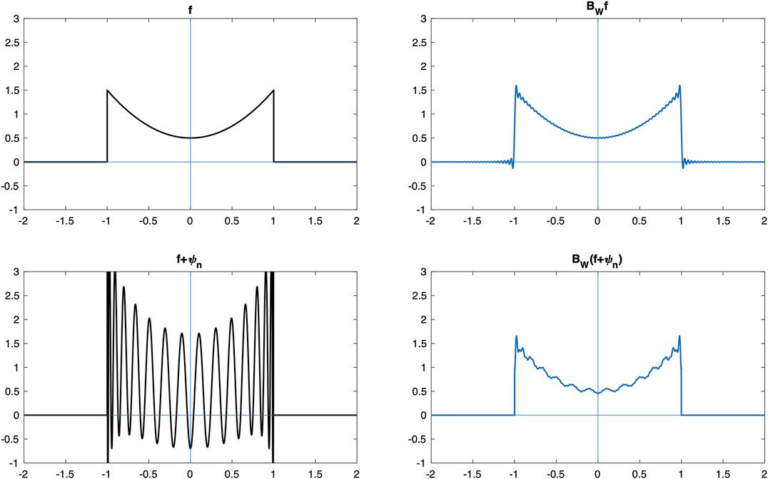
Remark 3.6. Consider the band-limiting operator $B_W$ acting on the space of time-limited functions $L^2\left(\mathcal{T}\right)$, where $\mathcal{T}=\left[-T,T\right]$. The eigenfunctions $\left\{{\psi }_j:j\in \mathrm{\mathbb{N}}\right\}$ of $B_W$ are the so-called prolate spheroidal wave functions (PSWFs) which are highly oscillating for big n. Suppose that the corresponding real eigenvalues $\left\{{\lambda }_n:n\in \mathrm{\mathbb{N}}\right\}$ are ordered by ${\lambda }_1>{\lambda }_2>\cdots \ge 0$. One can show that the amplitudes of the PSWFs ${\psi }_j$ satisfy a polynomial growth, while the eigenvalues ${\lambda }_j$ decay to zero exponentially [4]. Hence, a perturbation of a signal $f\in L^2\left(\mathcal{T}\right)$ by a PSWF ${\psi }_n$ causes a significant pointwise distortion of the original signal f (and therefore, of the phase ${\theta }_f$). If we define $h_n:=f+{\psi }_n$, then the band-limited version of $h_n$ is given by

$B_W{h}_n=f_W+{\lambda }_n{\psi }_n.$

Observing that ${\Vert {\lambda }_n{\psi }_n\Vert }_{\infty }\to 0$ exponentially as $n\to \infty$, we conclude that the distortion is negliglible after band limiting the perturbed signal $h_n$. In particular, this implies that, in general, one cannot expect a bound on the phase of $h_n$ and $B_W{h}_n$. This effect is visualized in Figure 1.

FIGURE 1

FIGURE 1. Perturbation of a signal f by a prolate spheroidal wave function ${\psi }_n$ before and after applying the band-limiting operator. To obtain the above visualization, we made use of approximation techniques of PSWFs as described in [1]

4. Phase-Preserving Operators

In Section 3, it has been shown under which conditions the phase of f is invariant under the action of the band-limiting operator, i.e., ${\theta }_f={\theta }_{B_{W}f}$. Moreover, we demonstrated that the equality of the two phases is not always possible, and we gave explicit examples for ${\theta }_f\ne {\theta }_{B_{W}f}$ by using perturbations by PSWFs. Therefore, the following question now comes up naturally.

Which operators $T:L^2\left(\mathrm{ℝ}\right)\to L^2\left(\mathrm{ℝ}\right)$ satisfy ${\theta }_f={\theta }_{Tf}$, for every $f\in L^2\left(\mathrm{ℝ}\right)$? Can we characterize those operators T?

In this section, we will give a precise characterization of operators on $L^2\left(\mathrm{ℝ}\right)$ which leave the phase invariant. The results will also be generalized to operators on $L^p\left(\mathrm{ℝ}\right),1\le p<\infty$. We start with a definition of a class of operators which we will call phase-preserving operators (PPO for short).

Definition 4.1. We call a bounded linear operator $T:L^2\left(\mathrm{ℝ}\right)\to L^2\left(\mathrm{ℝ}\right)$ to be phase-preserving if

${\theta }_f={\theta }_{Tf},$

for every $f\in L^2\left(\mathrm{ℝ}\right)$.

The following statement is an immediate consequence of the previous definition.

Lemma 4.2. If $T:L^2\left(\mathrm{ℝ}\right)\to L^2\left(\mathrm{ℝ}\right)$ is phase-preserving, then, for every $f\in L^2\left(\mathrm{ℝ}\right)$ with $f\ne 0$ a.e., there exists an a.e. unique function $p_f\ge 0$ such that $Tf=p_{f}f.$

Proof. Let $f\in L^2\left(\mathrm{ℝ}\right)$ with $f\left(t\right)\ne 0$, for a. e. $t\in \mathrm{ℝ}$. Then, for all $t\in \mathrm{ℝ}$ such that $f\left(t\right)\ne 0$ and $f\left(t\right)\ne \infty$, we have

$Tf\left(t\right)=e^{i{\theta }_{Tf}\left(t\right)}\left|Tf\left(t\right)\right|=\frac{e^{i{\theta }_{Tf}\left(t\right)}\left|Tf\left(t\right)\right|}{e^{i{\theta }_f\left(t\right)}\left|f\left(t\right)\right|}f\left(t\right)=\frac{\left|Tf\left(t\right)\right|}{\left|f\left(t\right)\right|}f\left(t\right),$

which implies

$p_f\left(t\right)=\frac{\left|Tf\left(t\right)\right|}{\left|f\left(t\right)\right|}.$

Since $\left\{t\in \mathrm{ℝ}\mathrm{:f}\left(t\right)=0\right\}{{\displaystyle \cup }}^{\text{}}\left\{t\in \mathrm{ℝ}\mathrm{:f}\left(t\right)=\infty \right\}$ is a zero set, the function $p_f$ is unique almost everywhere.

For $\varphi \in L^{\infty }\left(\mathrm{ℝ}\right)$, let the multiplication operator $M_{\varphi }:L^2\left(\mathrm{ℝ}\right)\to L^2\left(\mathrm{ℝ}\right)$ be defined by

$M_{\varphi }f=\varphi f.$

The function ϕ is called the symbol of the multiplication operator $M_{\varphi }$. Clearly, $M_{\varphi }$ is bounded with ${\Vert M\Vert }_{\varphi }={\Vert \varphi \Vert }_{\infty }$. It is obvious that if ϕ is real-valued with $\varphi \ge 0$ a.e., then $M_{\varphi }$ is phase-preserving. In the following, we will prove that the converse of this statement is true as well, i.e., for every PPO T, there exists a $\varphi \in L^{\infty }\left(\mathrm{ℝ}\right)$ with $\varphi \ge 0$ a.e. such that

$T=M_{\varphi }.$

In other words, the function $p_f$ from Lemma 4.2 is independent of f. To show this statement, we start by investigating the map $f\mapsto p_f$, where $p_f$ is defined as in Lemma 4.2.

Definition 4.3. Let $f:\mathrm{ℝ}\to \mathrm{ℂ}$ be measurable functions. We call f and g pointwise linear-independent if $\left(\text{Re}f\left(t\right),\text{Im}f\left(t\right)\right)$ and $\left(\text{Re}g\left(t\right),\text{Im}g\left(t\right)\right)$ are linear-independent vectors in ${\mathrm{ℝ}}^2$, for a.e. $t\in \mathrm{ℝ}.$

Lemma 4.4. Let $T:L^2\left(\mathrm{ℝ}\right)\to L^2\left(\mathrm{ℝ}\right)$ be phase-preserving, $f\in L^2\left(\mathrm{ℝ}\right)$ with $f\ne 0$ a.e., and $\lambda \in {\mathrm{ℂ}}^{\times }.$ Then,

$p_f=p_{\lambda f}.$

Moreover, if $g\in L^2\left(\mathrm{ℝ}\right)$ is a second function which is pointwise linear independent of f, then

$p_{f+g}=p_f=p_g.$

Proof. If $f\ne 0$ a.e., then $\lambda f\ne 0$ a.e. Due to linearity, we have

$\lambda p_{f}f=T\left(\lambda f\right)=p_{\lambda f}\lambda f.$

Therefore, $p_{\lambda f}=p_f.$ Now assume that $g\in L^2\left(\mathrm{ℝ}\right)$ is pointwise linear independent of f. Then, $f+g\ne 0$ a.e. since otherwise $f\left(t\right)$ and $g\left(t\right)$ would be pointwise linear-dependent on a set of measure greater than zero. Let $t\in \mathrm{ℝ}$ s.t. $f\left(t\right)$ and $g\left(t\right)$ are linear-independent. Due to the linearity of T, we obtain

$T\left(f+g\right)\left(t\right)=p_{f+g}\left(t\right)\left(f+g\right)\left(t\right)=p_f\left(t\right)f\left(t\right)+p_g\left(t\right)g\left(t\right).$

Linear independence implies $p_{f+g}\left(t\right)=p_f\left(t\right)=p_g\left(t\right).$ This equation holds for a.e. $t\in \mathrm{ℝ}.$

Suppose that $\mathcal{V}=\left\{f_1,f_2,\dots \right\}\subseteq L^2\left(\mathrm{ℝ}\right)$ is a system of functions with the property that, for every $n\in \mathrm{\mathbb{N}}$, there exists a $k\in \mathrm{\mathbb{N}}$ with $k\le n$ such that $f_n$ is pointwise linear independent of $f_k$. In this case, Lemma 4.4 implies that a PPO $T:L^2\left(\mathrm{ℝ}\right)\to L^2\left(\mathrm{ℝ}\right)$ is a multiplication operator on $\text{span}\mathcal{V}$. As a consequence, if $\mathcal{V}$ would be complete in $L^2\left(\mathrm{ℝ}\right)$, then T would be a multiplication operator by a simple extension argument. In the following, we will construct a system which satisfies exactly the conditions above. To do so, we consider the system of exponentials $\mathrm{ℰ}$ defined by the functions ${\chi }_c\left(t\right)=e^{2\pi ict},c\in \mathrm{ℝ}$. The set $\mathrm{ℰ}$ has the following property.

Lemma 4.5. Let ${\chi }_{c_1},\dots ,{\chi }_{c_n},{\chi }_{c_{n+1}}\in \mathrm{ℰ}$ be $n+1$ distinct exponentials and let ${\lambda }_1,\dots ,{\lambda }_n\in \mathrm{ℂ}$. We define $\ell :\mathrm{ℝ}\to \mathrm{ℂ}$ to be a nonzero linear combination of the first n exponentials:

$\ell :={\displaystyle \sum }_{j=1}^n{\lambda }_j{\chi }_{c_j}.$

Then, $\ell$ is pointwise linear independent of ${\chi }_{c_{n+1}}$

Proof. Without loss of generality, we may assume that ${\lambda }_j\ne 0$ for $j=1,\dots ,n.$ Let ${\lambda }_j=a_j+i{b}_j$ with $a_j,b_j\in \mathrm{ℝ}.$ Then,

$\text{Re}\ell \left(t\right)={\displaystyle \sum }_{j=1}^n{a}_j\text{cos}\left(2\pi c_{j}t\right)-b_j\text{sin}\left(2\pi c_{j}t\right)(6)$

and

$\text{Im}\ell \left(t\right)={\displaystyle \sum }_{j=1}^n{b}_j\text{cos}\left(2\pi c_{j}t\right)+a_j\text{sin}\left(2\pi c_{j}t\right).(7)$

We define the matrix

$M\left(t\right)=\left(\begin{array}{cc}\text{Re}\ell \left(t\right)& \text{cos}\left(2\pi c_{n+1}t\right)\\ \text{Im}\ell \left(t\right)& \text{sin}\left(2\pi c_{n+1}t\right)\end{array}\right).$

Then, $\ell$ and ${\chi }_{c_{n+1}}$ are pointwise linear-independent if $\text{det}M\left(t\right)\ne 0$, for almost every $t\in \mathrm{ℝ}.$ Plugging Eqs 6and7 into $M\left(t\right)$ and using the definition of the determinant as well as elementary trigonometric identities, we arrive at

$\text{det}M\left(t\right)={\displaystyle \sum }_{j=1}^n{a}_j\text{sin}\left(r_{j}t\right)-b_j\text{cos}\left(r_{j}t\right)$

with $r_j:=2\pi \left(c_{n+1}-c_j\right).$ In particular, $r_j\ne 0$, for every j, since $c_j$ was assumed to be distinct. We observe that $t\mapsto \text{det}M\left(t\right)$ can be extended to an entire function. Since zeros of entire functions form a discrete set with no accumulation point, it suffices to show that $t\mapsto \text{det}M\left(t\right)$ is not the zero function. To do so, we fix $k\in \left\{1,\dots ,n\right\}$ and let $R>0$. By using trigonometric identities, we observe that, for $j\ne k$, the term

$\left(a_j\text{sin}\left(r_{j}t\right)-b_j\text{cos}\left(r_{j}t\right)\right)\left(a_k\text{sin}\left(r_{k}t\right)-b_k\text{cos}\left(r_{k}t\right)\right)(8)$

is a sum of terms of the form

$\alpha \text{sin}\left(\left(r_j\pm r_k\right)t+\beta \right)$

with some $\alpha ,\beta \in \mathrm{ℝ}.$ Due to periodicity, this implies that there exists a $C>0$ such that

$\left|{{\displaystyle \int }}_{-R}^R\left(a_j\text{sin}\left(r_{j}t\right)-b_j\text{cos}\left(r_{j}t\right)\right)\left(a_k\text{sin}\left(r_{k}t\right)-b_k\text{cos}\left(r_{k}t\right)\right)dt\right|\le C,(9)$

for every $R>0$ and a constant $C>0$ independent of R. In case $j=k$, Eq. 8 becomes

${\left(a_k\text{sin}\left(r_{k}t\right)-b_k\text{cos}\left(r_{k}t\right)\right)}^2,$

which is a nonzero periodic function. Hence,

${{\displaystyle \int }}_{-R}^R{\left(a_k\text{sin}\left(r_{k}t\right)-b_k\text{cos}\left(r_{k}t\right)\right)}^{2}dt\to \infty (10)$

as $R\to \infty .$ Combining Eq. 9 with Eq. 10, it yields

${{\displaystyle \int }}_{-R}^R\text{det}M\left(t\right)\left(a_k\text{sin}\left(r_{k}t\right)-b_k\text{cos}\left(r_{k}t\right)\right)dt\to \infty$

as $R\to \infty$ In particular, $\text{det}M\left(t\right)$ is not the zero function.

We now give a characterization of PPO.

Theorem 4.6. Let $T:L^2\left(\mathrm{ℝ}\right)\to L^2\left(\mathrm{ℝ}\right)$ be a bounded linear operator. Then, T is phase-preserving if and only if there exists $\varphi \in L^{\infty }\left(\mathrm{ℝ}\right)$ with $\varphi \ge 0$ such that

$Tf=\varphi f,$

for every $f\in L^2\left(\mathrm{ℝ}\right).$ In other words, $T=M_{\varphi }.$

Proof. The fact that every multiplication operator $M_{\varphi }$ with $\varphi \ge 0$ is phase-preserving was discussed above. It remains to show the converse. We fix $f\left(t\right)=e^{-\pi t^2}$; then, $f\in L^2\left(\mathrm{ℝ}\right)$ and $\mathrm{ℱ}f\left(\xi \right)\ne 0$, for every $\xi \in \mathrm{ℝ}$. Wiener’s Tauberian theorem [8] implies that $\text{span}\left\{f\left(\cdot -c\right)\right|c\in \mathrm{ℝ}\}$ is dense in $L^2\left(\mathrm{ℝ}\right)$. Since the Fourier transform is an isometry and $\mathrm{ℱ}f=f$, the set

$Q:=\text{span}\left\{M_{-c}f\right|c\in \mathrm{ℝ}\}$

is dense in $L^2\left(\mathrm{ℝ}\right)$. Let $g,h\in Q$ with $g\ne h$. Then,

$g=\left({\displaystyle \sum }_{j\in A}{\lambda }_j{\chi }_{-c_j}\right)f$

and

$h=\left({\displaystyle \sum }_{i\in B}{\mu }_i{\chi }_{-c_i}\right)f$

for some $c_j,c_i\in \mathrm{ℝ}$, ${\lambda }_j,{\mu }_i\in \mathrm{ℂ}$, and finite subsets $A,B\subset \mathrm{\mathbb{N}}$. We choose an exponential ${\chi }_{-c_k}$ with $k\notin A$ and $k\notin B$. Since f is positive everywhere, Lemma 4.5 implies that ${\chi }_{-c_k}f$ is pointwise linear independent of both g and h. Lemma 4.4 implies that $p_h=p_g.$ Since g and h are arbitrary, we obtain a function $\varphi \in L^{\infty }\left(\mathrm{ℝ}\right)$ with

$Tg=\varphi g$

for every $g\in Q.$ We show that $\varphi \in L^{\infty }\left(\mathrm{ℝ}\right).$ Assume the contrary, i.e., ϕ is not essentially bounded. Then, for every $n\in \mathrm{\mathbb{N}}$ the set

$A_n:=\left\{t\in \mathbb{R}:\left|\varphi \left(t\right)\right|\ge n\right\}$

has a positive Lebesgue measure. We now choose $f_n\in L^2\left(\mathrm{ℝ}\right)$ with $f_n=0$ on $\mathrm{ℝ},A_n$ and ${\left|\left|f_n\right|\right|}_2=1$. Furthermore, we choose $q_n\in Q$ such that

${\Vert f_n-q_n\Vert }_2\le \frac{1}{n}.$

which is possible due to density of Q in $L^2\left(\mathrm{ℝ}\right).$ We estimate the $L^2$-norm of $q_n$ as follows:

${\left|q_n\right|}_{L^2\left(A_n\right)}^2={\Vert q_n\Vert }_{L^2\left(\mathrm{ℝ}\right)}^2-{\left|q_n\right|}_{L^2\left(\mathrm{ℝ},A_n\right)}^2$

$\ge {\left(1-\frac{1}{n}\right)}^2-\left(f_n-q_{n{L}^2\left(\mathrm{ℝ}\right)}^2-f_n-q_{n{L}^2\left(A_n\right)}^2\right)\ge 1-\frac{2}{n}$

With this choice of $q_n$, we obtain the following estimate:

$T^2{\left|q_n\right|}_2^2\ge {\left|\varphi q_n\right|}_2^2\ge n^2\underset{A_n}{{\displaystyle \int }}|q_n{|}^2\ge n^2\left(1-\frac{2}{n}\right)$

Because $q_{n_2}\le 1+\frac{1}{n}$, we see that

$T\ge n{d}_n$

where $\left(d_n\right)$ is a sequence with $d_n\to 1$. This is a contradiction to the boundedness of T. Consequently, $\varphi \in L^{\infty }\left(\mathrm{ℝ}\right)$ and

$T=M_{\varphi }$

on Q. Since Q is a dense subset of $L^2\left(\mathrm{ℝ}\right)$, we have $T=M_{\varphi }$ on the closure of Q, i.e., on $L^2\left(\mathrm{ℝ}\right)$.

The characterization of PPOs in Theorem 4.6 was stated in the space $L^2\left(\mathrm{ℝ}\right)$. The first property we used in the proof was the pointwise linear independence of exponentials. This condition is purely algebraic and does not depend on the structure of $L^p\left(\mathrm{ℝ}\right)$. The second crucial property we needed was the density of modulations of a positive function $f\in L^2\left(\mathrm{ℝ}\right)$ (in our case, f was a Gaussian) which was based on Wiener’s Tauberian theorem. Equivalently, this means that the set of exponentials

$\mathrm{ℰ}:=\left\{e^{2\pi ic}\right|c\in \mathrm{ℝ}\}(11)$

is complete in $L^2\left(\mathrm{ℝ},\mu \right)$, where $\mu =fdx$. In view of this reformulation, the characterization of PPOs can be generalized to operators on $L^p\left(\mathrm{ℝ}\right)$ which provided that the set of exponentials $\mathrm{ℰ}$ is complete in $L^p\left(\mathrm{ℝ},\mu \right)$. It is well known that this is true for every Borel measure µ on $\mathrm{ℝ}$ which is positive and finite.

Theorem 4.7. Let µ be a positive, finite Borel measure on $\mathrm{ℝ}$. We denote by $\mathrm{ℰ}$ the set of exponentials as defined in Eq. 11. Then, $\mathrm{ℰ}$ is complete in $L^p\left(\mathrm{ℝ},\mu \right)$ for every $p\in \left[1,\infty \right)$.

Proof. Assume by contradiction that $\mathrm{ℰ}$ is not complete in $L^p\left(\mathrm{ℝ},\mu \right)$. Then, there exists an $0\ne f\in L^p\left(\mathrm{ℝ},\mu \right),\overline{\text{span}}\mathrm{ℰ}$. Moreover, the Hahn–Banach theorem implies that there is a continuous linear functional $\ell \in L^p{\left(\mathrm{ℝ},\mu \right)}^{\text{*}}$ such that

$\ell {|}_{\overline{\text{span}}\mathrm{ℰ}}=0,\ell \left(f\right)=\text{dist}\left(f,\overline{\text{span}}\mathrm{ℰ}\right)\ne 0.(12)$

By the Riesz representation theorem, the functional $\ell$ has the form

$\ell \left(g\right)={\displaystyle {\int }_{\mathrm{ℝ}}g\left(t\right)m\left(t\right)d\mu \left(t\right)}$

for some $m\in L^q\left(\mathrm{ℝ},\mu \right)$ and every $g\in L^p\left(\mathrm{ℝ},\mu \right)$, where q is the Hölder conjugate exponent of p. The identities in Eq. 12 imply that

${\displaystyle {\int }_{\mathrm{ℝ}}m\left(t\right)e^{2\pi ict}d\mu \left(t\right)=0}$

for every $c\in \mathrm{ℝ}$. Let $\tau :=m\mu$. Then, τ is a finite signed measure on $\mathrm{ℝ}$ with the property that its Fourier–Stieltjes transform is zero:

$\widehat{\tau }=0.$

By the uniqueness theorem of the Fourier–Stieltjes transform of measures, we have $\tau =m\mu =0$ which implies that $\ell =0$, contradicting Eq. 12.

Corollary 4.8. Let $p\in \left[1,\infty \right)$ and $T:L^p\left(\mathrm{ℝ}\right)\to L^p\left(\mathrm{ℝ}\right)$ a bounded linear operator. Then, T is phase-preserving if and only if T is a multiplication operator with nonnegative symbol $\varphi \ge 0$.

Proof. It is clear that a multiplication operator on $L^p\left(\mathrm{ℝ}\right)$ with a nonnegative symbol is a PPO. For the other directions, we fix $f\left(t\right)=e^{-\pi t^2}$. Since f is a Schwartz function, it lies in $L^p\left(\mathrm{ℝ}\right)$, for every $1\le p\le \infty$. Consider the measure

$\mu =fdx$

where $dx$ stands for the Lebesgue measure. Clearly, µ is a finite, positive Borel measure on $\mathrm{ℝ}$. Theorem 4.7 implies that the set of exponentials is complete in $L^p\left(\mathrm{ℝ},\mu \right)$, which is equivalent to say that

$Q=\text{span}\left\{M_{c}f\right|c\in \mathrm{ℝ}\}$

is dense in $L^p\left(\mathrm{ℝ}\right)$. The proof now follows the lines of the proof of the characterization theorem in $L^2\left(\mathrm{ℝ}\right)$ by replacing the $L^2$-norm by the $L^p$-norm.

We finish this section by establishing a relation between the previous characterization theorems and Section 3, where we obtained bounds on the phase of a compactly supported function f and the phase of its band-limited version $f_W$.

Assume that $\varphi \in L^1\left(\mathrm{ℝ}\right)$ is nonnegative with $\mathrm{ℱ}\varphi \in L^1\left(\mathrm{ℝ}\right)$. Let $M_{\varphi }$ be the corresponding multiplication operator and for $W>0$, let $B_W$ be the band-limiting operator. By Young’s inequality, the operator $S_{\varphi }:L^2\left(\mathrm{ℝ}\right)\to L^2\left(\mathrm{ℝ}\right)$,

$S_{\varphi }h=\mathrm{ℱ}\varphi \text{*}h$

is well-defined and bounded. It follows that

$M_{\varphi }f={\mathrm{ℱ}}^{-1}\left(\mathrm{ℱ}\varphi \text{*}\mathrm{ℱ}f\right)={\mathrm{ℱ}}^{-1}{S}_{\varphi }\mathrm{ℱ}f.$

Similar to Definition 3.1, we say that a function $f\in L^2\left(\mathrm{ℝ}\right)$ is (strictly) ${\epsilon }_{\mathcal{W}}$-localized with respect to the $L^2$-norm if ${\left|\left|f-R_{W}f\right|\right|}_2<{\epsilon }_{\mathcal{W}}.$ As defined before, $\mathcal{W}$ denotes the interval $\left[-W,W\right]$. Now, suppose that the Fourier transform of a given compactly supported function $f\in L^2\left(\mathcal{T}\right)$ is (strictly) ${\epsilon }_{\mathcal{W}}$-localized with respect to the $L^2$-norm, i.e.,

${\left|\left|\mathrm{ℱ}f-R_W\mathrm{ℱ}f\right|\right|}_2<{\epsilon }_{\mathcal{W}}.$

We define $\delta :={\epsilon }_{\mathcal{W}}-\mathrm{ℱ}f-R_W\mathrm{ℱ}{f}_2>0$ and choose ϕ in such a way that

${\left|\left|\mathrm{ℱ}\varphi \text{*}\mathrm{ℱ}f\right|\right|}_2\le \delta .$

The existence of such a ϕ easily follows from the fact that the Gauss kernel is an approximate identity. Combining the two previous inequalities, we obtain the bound

${\left|\left|M_{\varphi }f-B_{W}f\right|\right|}_2={\Vert S_{\varphi }\mathrm{ℱ}f-R_W\mathrm{ℱ}f\Vert }_2\le {\epsilon }_{\mathcal{W}}.$

This proves the following statement.

Corollary 4.9. Let $f\in L^2\left(\mathcal{T}\right)$ be such that its Fourier transform is (strictly) ${\epsilon }_{\mathcal{W}}$-localized in the $L^2$-sense. Then, there exists a nonnegative function $\varphi \in L^1\left(\mathrm{ℝ}\right)\cap L^{\infty }\left(\mathrm{ℝ}\right)$, for which

${\left|\left|M_{\varphi }f-B_{W}f\right|\right|}_2\le {\epsilon }_{\mathcal{W}}.(13)$

Note that an $L^2$-localization of f can be achieved in an analogous manner to Section 3. Suppose that $f\in C^{n+1}\left(\mathrm{ℝ}\right)$ and that we have control over the total variation norm of $f^{\left(n\right)}$. We then obtain an ${\epsilon }_{\mathcal{W}}$-localized function (in the $L^1$-sense), and from the control over the BV-norm, we can assume that $\left|\widehat{f}\left(\xi \right)\right|\le 1$, for every $\left|\xi \right|\ge W$. This yields

${\left|\left|\widehat{f}-R_W\widehat{f}\right|\right|}_2\le {\Vert \widehat{f}-R_W\widehat{f}\Vert }_1\le {\epsilon }_{\mathcal{W}}.$

We conclude that if f satisfies the assumptions derived in Section 3 (regularity and control over the total variation norm) which yielded a bound on the phase distance $\left|\theta -{\theta }_W\right|$, then the band-limiting operator $B_W$ is close to a multiplication operator (in the $L^2$-sense).

5. Conclusion

In this article, we were concerned with phase distortions caused by band limiting a compactly supported signal. This problem naturally arises in the field of optics such as diffraction imaging. Precise localization and regularity conditions were derived for which a bound on the phase of the input signal and the band-limited signal is achievable. The class of operators which leave the phase of any input signal invariant was characterized as multiplication operators with nonnegative symbol.

Data Availability Statement

The original contributions presented in the study are included in the article, and further inquiries can be directed to the corresponding author.

Author Contributions

Both authors listed have made a substantial contribution to the work and approved it for publication.

Funding

The work was partially funded by the Helmholtz Association under the project Ptychography4.0. The open-access publication fees are payed by the University of Vienna via the open-access publishing agreement between Frontiers and the University of Vienna. The corresponding author (Lukas Liehr) is affiliated to the University of Vienna.

Conflict of Interest

The authors declare that the research was conducted in the absence of any commercial or financial relationships that could be construed as a potential conflict of interest.

Acknowledgments

The authors thank the reviewers for their valuable comments which were very helpful to improve the paper.

References

1. Bonami, A, and Karoui, A. Uniform approximation and explicit estimates for the prolate spheroidal wave functions. Constr Approx. (2016). 43:15–45. doi:10.1007/s00365-015-9295-1

CrossRef Full Text | Google Scholar

2. Donoho, DL, and Stark, PB. Uncertainty principles and signal recovery. SIAM J Appl Math. (1989). 49:906–31. doi:10.1137/0149053

CrossRef Full Text | Google Scholar

3. Mallat, S. A wavelet tour of signal processing. 2nd ed. Cambridge, MA: Academic Press (1999).

Google Scholar

4. Osipov, A, Rokhlin, V, and Xiao, H. Prolate spheroidal wave functions of order zero. Mathematical tools for bandlimited approximation. New York, NY: Springer US (2013).

Google Scholar

5. Slepian, D. Some comments on fourier analysis, uncertainty and modeling. SIAM Rev. (1983). 25(3):379–93. doi:10.1137/1025078

CrossRef Full Text | Google Scholar

6. Slepian, D, and Pollak, HO. Prolate spheroidal wave functions, fourier analysis and uncertainty - I. Bell Syst Tech J (1961). 40(1):43–63. doi:10.1002/j.1538-7305.1961.tb03976.x

CrossRef Full Text | Google Scholar

7. Stein, EM, and Weiss, G. Introduction to fourier analysis on Euclidean spaces, Vol. 32. Princeton, NJ: Princeton University Press (1971).

Google Scholar

8. Wiener, N. Tauberian theorems. Ann Math. (1932). 33(1):1–100. doi:10.2307/1968102

CrossRef Full Text | Google Scholar

9. Zhu, K. Operator theory in function spaces, Vol. 138. Mathematical Surveys and Monographs, American Mathematical Society (2007).

Google Scholar