Application of a Susceptible, Infectious, and/or Recovered (SIR) Model to the COVID-19 Pandemic in Ecuador

1. Introduction

The coronavirus disease 2019 (COVID-19) pandemic that is wreaking havoc in healthcare systems worldwide is caused by severe acute respiratory syndrome coronavirus 2 (SARS-CoV-2) infection. Several phylogenetic studies have determined the origin of this zoonotic virus and, simultaneously, the potential reservoirs and amplifying species (especially mammals) [1–3].

The first report of SARS-CoV-2 infection was in December 2019 in Wuhan (Hubei Province, China). Worldwide spread of SARS-CoV-2 was inevitable due to its easy dissemination (as droplets), apparently low mortality, and high incidence of asymptomatic cases (≥15.8% of infected people) [1–5].

In <3 months, 60% of countries reported COVID-19 cases, particularly in Europe (e.g., Italy, Spain). Then, SARS-CoV-2 infection was documented in North America and, one week later, in Brazil, Ecuador, and Chile.

For COVID-19, lethality has been estimated to be 4–6%, mortality to be 1–1.5%, and severe illness to occur in ≥4.7% of diagnosed cases. The recovery time has been estimated to range from 8 to 11.5 days, but it is related to multiple factors [6–8].

The Ministry of Public Health (MSP) of Ecuador reported the first case of COVID-19 on February 27, 2020. It was an Ecuadorian woman who returned from Spain to Guayaquil on a commercial flight and had a welcoming party. Then, other cases at the northern (Tulcan) and southern (Machala) borders appeared (arising potentially from Colombia and Peru, respectively) [8]. By the beginning of June, according to official reports, there were ≥43,120 confirmed cases, with a higher prevalence in people aged 21–60 years, lethality of 4–7%, and a mortality rate (<1%) [8, 9].

Mathematical models such as the Susceptible, Infectious, and/or Recovered (SIR) model are used to predict different scenarios related to epidemiologic factors and possible outcomes to assess epidemic spread. The reproduction number (R0) is used to estimate the capacity of viral transmission from one person to another. The effective reproduction number (Re or Rt) refers to the number of infected people in a specific time interval based on the R0. The susceptible fraction (Fso) takes into account the percentage of infected people that might exist in an epidemic. These indices show how a population and a virus are related to make predictions and consider the consequences at a given moment [8, 10, 11].

We aimed to generate SIR models based on data provided by the Ecuadorian MSP to estimate R0, Rt, Fso, time in quarantine, and the required percentage of immunized people to consider a reduction in the total incidence of COVID-19 in Ecuador. This strategy would allow the creation of a new SIR model readily without the need to have a large volume of regional data or national data. The possibility of developing retrospective and predictive models in this or other conditions based on an R0 calculation (observed here as a dynamic value) and the generation of a dynamic Rt value that will serve as a reference to make decisions in real-time, along with another type of model for quarantine and immunization, would be very helpful.

2. Methodology

2.1. Data Source

The data used for these models were from daily reports produced by the MSP. The data comprised of cumulative cases, new cases, excluded cases, deceased cases, cases who recovered from COVID-19, number of testing samples, and samples already collected but waiting to be processed from day-1 to day 30 of the epidemic (https://www.gestionderiesgos.gob.ec/informes-de-situacion-covid-19-desde-el-13-de-marzo-del-2020/) [9]. Values were taken from day 1 to day 30 of the epidemic considering the range with the highest reliability of data.

The SIR model, predictions/estimations, and tabulation data were processed using Excel™ within Office™ v16.37 (Microsoft, Redmond, WA, United States). Model parameters were verified using Vensim™ v8.0.9 (Salisbury, United Kingdom) and RStudio™ v4.0 (R Foundation for Statistical Computing, Vienna, Austria). Graphs were generated using Prism™ v8.4.2 (GraphPad, San Diego, CA, United States).

2.2. Estimated Infection Rate for the COVID-19 Epidemic in Ecuador

We used the parameters related to the number of individuals infected per day, the trend of the epidemic, mean number of samples processed, and samples waiting to be processed to determine the percentage of “true” work carried out by the MSP. Then, we compared the number of daily infected cases and estimated the rate of increase (cases/day). This was done using Eq. 1, in which the numerator is the number of reported cases in a final period of time and the denominator is the number of reported cases in an initial time [12, 13].

$rateofincrease\left[\frac{cases}{day}\right]=\frac{Infectedt2}{Infectedt1}(1)$

$contagionrate=\left(1-rateofincrease\right)\ast 100\%(2)$

The result using Eq. 1 revealed whether the number of cases increased or not from 1 day to another, and also predicted the number of new cases for the next day. Thus, it also estimated the daily rate of contagion (Eq. 2), and the percentage of contagion in a certain period, based on the rate of increase. Both rates enabled the observation of dynamic behavior with R0 and Rt.

2.3. Calculation of the Minimum Number of Cases Required to Generate the COVID-19 Epidemic in Ecuador

A mathematical model based on sigmoid curves was applied to estimate the minimum number of cases required to generate an epidemic (“community infection”). To calculate the constants for the equation, two methods were employed. First, Eq. 3 (K1) was obtained from the curve for the number of positive case reported by the MSP using logarithmic regression, where t is the time of infection, and I is the number of people infected in time t. Second, Eq. 4 (K2) was considered as a differential logarithm regarding time, where Ti is the initial infection time, Tf is the final infection, If denotes finally-infected individuals and Ii denotes initially-infected people in an estimated period of time [14].

$K1=\frac{{\displaystyle \sum Ln\left(t\right)-Ln\left(I\right)-\frac{{\displaystyle \sum Ln\left(t\right)\ast {\displaystyle \sum Lb\left(I\right)}}}{n}}}{{\displaystyle \sum {\left(Ln\left(t\right)\right)}^2-\frac{{\displaystyle \sum {\left(Ln\left(t\right)\right)}^2}}{n}}}(3)$

$K2=\frac{Ln\left(If\right)-Ln\left(Ii\right)}{Tf-Ti}(4)$

For K1 all the study data was used and in K2 data were from shorter ranges. Then, K2 provides daily evolution while K1 provides a general view of the epidemic. To calculate It (Eq. 5) (the number of infections over time in an epidemic), Ic was the number of infections present when the epidemic started. Based on the results, K1 (Eq. 3) was 0.1972, and K2 (Eq. 4) was 0.2386.

$It=\left[\frac{1}{1+Ic{e}^{-kt}}\right]I{c}^2(5)$

2.4. Duration of Quarantine

To determine the duration of quarantine and its subsequent removal, we needed to calculate the recovery time of the population. Hence, we took the minimum number of cases after the first recovery of COVID-19, and a hypothetical daily peak of infections (for our purpose this was considered to be 100 daily cases [15]) and a threshold of cases after this peak for considering lifting the quarantine. Hence, when this number of infected cases was reached, with no increase in the last few days, quarantine could be lifted. We assumed that all the daily reports from the MSP detailed the maximum number of cases, so we would know how long it would take for the recovery of these infected individuals [14].

$It=\frac{If}{1+\left(If-\mathit{Reo}\right)e^{-kIft}}(6)$

$k=Ln\left[\frac{\frac{If}{It}+1}{If}\right](7)$

$td=\frac{Ln\left[\frac{\frac{If}{Ir}-1}{If}\right]}{k}(8)$

In Eq. 6, It is the number of recoveries in a period, If is the maximum number of infections in a particular period, Reo is the number of people who recovered on day-0 after reaching the maximum number of infected individuals (usually 1). In Eq. 7, k is the constant of proportionality. In Eq. 8, td is the duration of quarantine, Ir is the maximum number of infected people minus the threshold of 100 infected individuals [15] needed for lifting the quarantine (Ir = If − 100) and If is the maximum of cases for each day of quarantine.

2.5. SIR Models for COVID-19

We wished to model and predict the behavior of the COVID-19 epidemic in Ecuador. Hence, we took into account three mathematical models based on SIR, differed in the use of different parameters for the equations and the calculation of R0, where we did not consider the rate of asymptomatic cases (not a well-established value at the time of analyses).

The first model (Eqs 9–16) was based on the number of infections generating new cases. The parameters for construction were the recovery rate (95%), mortality rate (5%), time needed for recovery (17 days), R0 (taken from international databases [5], and assuming that 40% of the population was under total quarantine (that is equivalent to 4% less probability of becoming infected). N was the total population of Ecuador and the R0 was the ratio between the number of infected people and the number of people who recovered and those who died (Eqs 13, 16) [13, 16–18].

$\%P=\frac{NCoM}{IiTDSi}(9)$

$CoM=\frac{IiTDSi}{N\%P}(10)$

$\mathit{Re}=Ii\ast \left(\frac{TR}{DI}\right)(11)$

$M=Ii\ast \left(\frac{TM}{DI}\right)(12)$

$R0=\frac{CoM}{\left(\mathit{Re}+M\right)}(13)$

$Rt=\frac{CoM\left(t\right)}{\left(\mathit{Re}\left(\mathit{t}\right)+M\left(t\right)\right)}(14)$

$dRt=R0\ast \left(\frac{1}{1+e^{\left(\frac{So}{N}\right)}}\right)\ast \left(\frac{So}{N}\right)\ast \left(e^{\left(\frac{So}{N}\right)}\right)(15)$

$R0m=\sqrt[n]{R01\ast R02\ast R0n}(16)$

Sf (Eq. 17) represents the number of vulnerable individuals, If (Eq. 23) is the number of infected people, Rf (Eq. 21) is the number of people who recovered from COVID-19, Mf (Eq. 22) is the number of people who died; all of these parameters were taken after a certain period of time. DI represents the duration of illness in days, TD (Eq. 10) is the percentage of infections (R0), %P (Eq. 9) is the probability of becoming infected, TR (Eq. 11) is the percentage of people who recovered, TM (Eq. 12) is the percentage of individuals who died, and Rt (Eqs 12, 15) is the R0 that varies through time and the function of infected people.

The second model (Eqs 17–26) takes into consideration differential equations from a standard model that were integrated subsequently with national data where the percentage of people who recovered (γ) (Eq. 17) was 95%, mortality (μ) (Eq. 22) was 5%, and the time for recovery (TR) (Eqs 9, 11, 20) was 17 days. To calculate R0 for Ecuador, we considered standard calculations (Eqs 21, 26). Rt (Eqs 14, 15, 24) was based on the variation in the percentage of susceptible people during a particular time, and p (Eq. 17) was the relationship between the number of people who recovered from COVID-19 and the infection rate [13, 19].

$p=\frac{\gamma }{\beta }(17)$

$p=\frac{N-Sf}{Ln\left(\frac{\gamma N-\gamma R}{\gamma So}\right)}(18)$

$R0=\frac{\beta }{\gamma }So(19)$

$Sf=So{e}^{-\left[\frac{N-So}{p}\right]}(20)$

$Rf=\left(\frac{\gamma }{TR}\right)Ro(21)$

$Mf=\mu Ii(22)$

$If=Sf=Ii-Ri-Mi(23)$

$Rt=Ro\ast e^{\left(\frac{So}{N}\right)}(24)$

$dRt=R0\ast \left(\frac{1}{1+e^{\left(\frac{So}{N}\right)}}\right)\ast \left(\frac{So}{N}\right)\ast e^{\left(\frac{So}{N}\right)}(25)$

$R0m=\sqrt[n]{R01\ast R02\ast R0n}(26)$

The third model (Eqs 27–36) was based on the infection rate calculated with the equation for the rate of increase, so the β value (Eq. 27) was assigned to it. For the recovery rate (γ), it was considered that 17 days was the minimum time required to recover, and a 3% mortality percentage (μ) in accordance to the MSP report [10, 13].

$\beta =1-rate(27)$

$\gamma =\frac{1}{recuperationtime}(28)$

$R0=\frac{\beta }{\left(\gamma +\mu \right)}(29)$

$Infection\left(Con\right)=\beta \ast Ii\ast R0\ast \left(\frac{So-Ii}{N}\right)(30)$

$If=So-Con-\mathit{Re}-Mu(31)$

$\mathit{Re}cuperation\left(\mathit{Re}\right)=If\ast \gamma (32)$

$Dead\left(Mu\right)=If\ast \mu (33)$

$Rt=Ro\ast e^{\left(\frac{So}{N}\right)}(34)$

$dRt=R0\ast \left(\frac{1}{1+e^{\left(\frac{So}{N}\right)}}\right)\ast \left(\frac{So}{N}\right)\ast \left(e^{\left(\frac{So}{N}\right)}\right)(35)$

$R0m=\sqrt[n]{R01\ast R02\ast R0n}(36)$

2.6 Variation of the SIR Model With Different Values of R0

Taking into consideration the first proposed SIR model (Eqs 9–16), we generated different R0 values (Eqs 13, 16) and observed their behavior during a particular time. This strategy allowed for the ascertainment of how Rt and the epidemic cycle were related so that we could observe it and identify possible “bottlenecks”, when the number of susceptible people decreased (for whatever reason). Simultaneously, we compared the derivative of Rt (Eq. 15), which allowed us to observe the maximum number of infections when Rt varied, and worked to adjust a national R0 [14]. For model validation, we applied a difference between the curve for infected people (from the MSP report) and the number of infections generated with the three SIR models. Then, the curve (of these three models) that best fits to the real data reported by the MSP, was selected for further analysis [14].

2.7. Susceptible Factors and the Minimum Percentage Required for Immunization Using Rt

For the Rt of each model, we calculated the susceptible factor (Fso) (Eq. 37). This strategy allowed us to observe the highest percentage of infections (based on the variation in Rt) to generate a threshold that estimated the direction of the epidemic and where R0 was located in Ecuador [10, 19]. With Fso and R0 generated in each model, we could predict the minimum percentage (%Pi,v) (Eq. 38) required for immunization (by vaccination or herd immunity) to stop COVID-19 spread [10, 19].

$fSo\left(t\right)=1-e^{-Rt}(37)$

$\%Pi,v=1-\frac{1}{R0}(38)$

2.8. Vaccination and Immunization

After the derivation of %Pi,v from Eq. 38, we considered the incorporation of the Rt toward the population (N). Considering the variation in infection, we could recognize how long it would take for a vaccination strategy to obtain results and stop infection. We could also observe the number of immunized individuals and those who would not be infected during a particular time [10, 18, 20].

$\mathit{Im}munizatepopulation\left(Piz\right)=N\ast \left(1+\left(\frac{1}{2R{t}^2}\right)\right)(39)$

$Infectedpopulation\left(Pif\right)=N-N\ast \left(1+\left(\frac{1}{2R{t}^2}\right)\right)(40)$

3. Results

Upon analyses of all the reported data by the MSP, a marked delay in sample processing was noticed (40% CI = ±0.0035) and an increase in the number of new daily cases of 28.5% (CI = ±0.00146) was reported. Hence, the infection curve was delayed in 28.5% of cases (∼40% of undetermined cases). This observation was confirmed when the rate of increase per day remained the average between the number of delayed samples and number of reported cases. This resulted in 1.20 reported cases per day (CI = ±0.0103). When we analyzed the number of cases with COVID-19 reported by the MSP, there was a 30% delay in confirmatory diagnose. This problem was most evident at day 33 of the epidemic when there was 60% delay in confirmatory diagnoses (Figure 1).

FIGURE 1

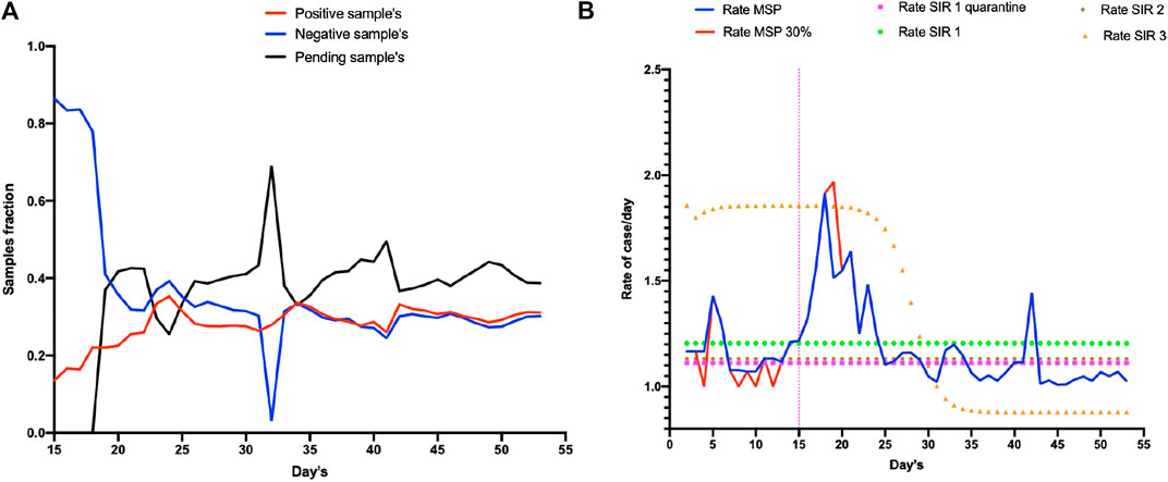
FIGURE 1. Report of the COVID-19 epidemic in Ecuador in January 2020. Section (A) shows the diagnoses of people in Ecuador from 15 February to 23 April 2020 (15 at 55 days of the epidemic) whereby red denotes the number of positive cases, blue denotes the number of negative cases, and black the number of samples. (B) shows in blue line the increase rate of cases in MSP report, red line represents the possible real number of reported cases (including 30% delay in confirm diagnose). The model SIR 1 showed the more accurate tendency (orange line).

We used K values (Eqs 3, 4) to determine the minimum number of cases required to generate an epidemic in Ecuador. In our simulation using K1, five cases were needed for an epidemic in Ecuador. Also, the model using K2 showed that with six cases, an exponential communitarian infection was possible (Figure 2), and that recovery from COVID-19 could take 18 days (CI = ± 0.0945).

FIGURE 2

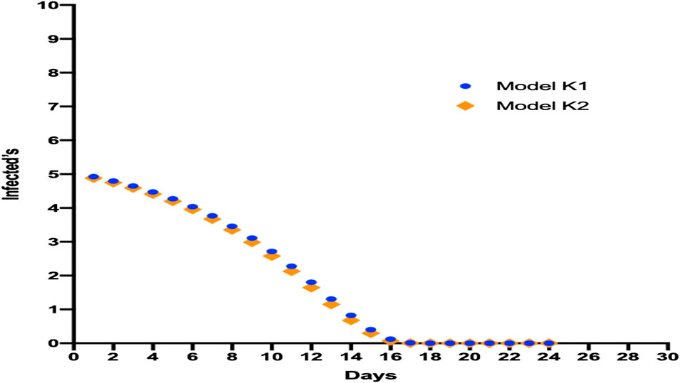
FIGURE 2. Model for the minimum number of cases required for an epidemic in Ecuador showing different simulations with various K constants for observing this number, communitarian infection, and the average time needed for recovery.

While observing the trend in the increase in infected cases, one key question was how long the quarantine should last until there were 100 infected cases. We calculated that quarantine should be lifted after approximately 80–110 days (CI = ±0.2001) because the maximum number of cases had been reached (Figure 3).

FIGURE 3

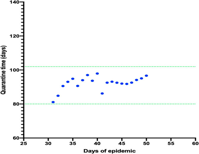
FIGURE 3. Model for the number of days required for quarantine and the maximum number of daily cases. It was observed that the number of days necessary to finish the quarantine remained the same despite the increasing number of cases daily.

Simultaneously with obtaining results, we generated three SIR models with variation of some parameters to obtain R0 and observed which model was the best fit.

When the number of infected people was compared for each model, model 1 (SIR 1) obtained the closest values to the true situation. Hence, we chose model 1 to observe the dynamic in cases once quarantine had been implemented (Figure 4). Using this model, R0 = 2.2 (CI = −1.644, +2.75). Importantly, with each model, an R0 value was generated so a different Rt analysis was undertaken to detect the appearance of a bottleneck in a susceptible population. We found that, for each model, the R0 was between 1 and 3 (CI = −1.865, +1.974) (Table 1).

FIGURE 4

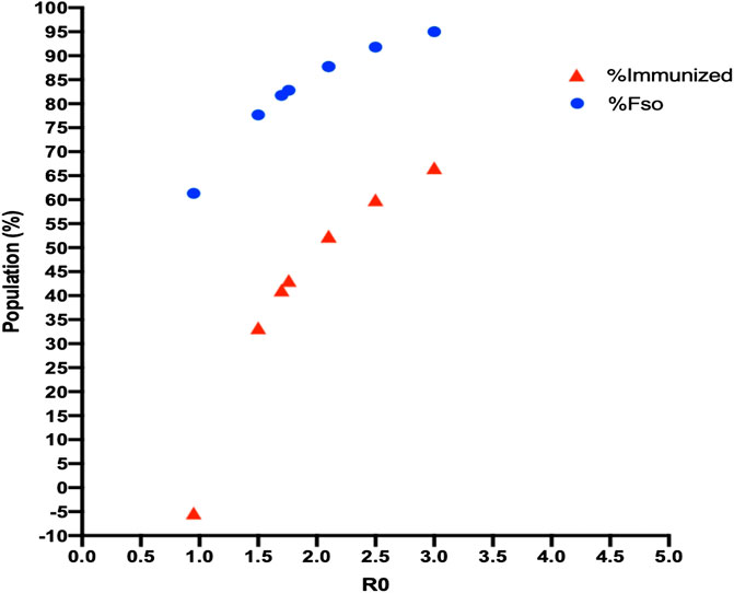
FIGURE 4. Fso and herd-immunity values with R0 for each model. An increase in R0 for each SIR model led to an increase in the infected population and herd immunization, but neither of these values reached 100% of the population.

TABLE 1

TABLE 1. R0 values generated with three SIR models showing the maximum number of people who may be infected (Fso), and herd immunity for each model.

Using these values, we calculated the maximum number of people susceptible to SARS-CoV-2 infection for each R0 value (95.02%, CI = ±1.27). The same calculation showed that a maximum of 66.67% (CI = ±2.70) of the same population would need to be immunized to stop the epidemic (Figure 5).

FIGURE 5

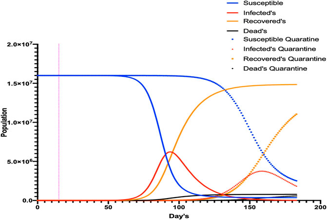
FIGURE 5. SIR1 model with modified parameters for quarantine. Different simulations were undertaken for COVID-19, with and without quarantine. The number of infected individuals decreased but the duration of infectivity was prolonged by >200 days.

When quarantine parameters were generated with SIR 1, the peak of the maximum number of infected individuals would be reached on day 154 of the epidemic (65 more days than if quarantine was not applied). The number of new cases would decrease (64.6%, CI = ±2.35) but not disappear, demonstrating that when the quarantine time increased, the number of infected cases was redistributed. This phenomenon was observed when the different Rt values (generated by a variation in parameters) were analyzed (Figure 6) and demonstrated that, for each unit increase in Rt, the epidemic would increase by 10 days (CI = ±0.295).

FIGURE 6

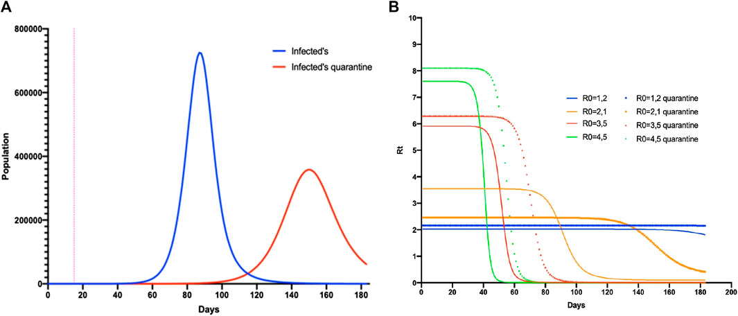
FIGURE 6. SIR1 model comparing the parameters regulated with quarantine. (A) The number of infected people without quarantine (blue) and with quarantine (red). (B) Simulation of Rt in the SIR1 model varying the parameters with and without quarantine over the duration of the epidemic.

To confirm the obtained R0 with SIR 1, we analyzed the variation in Rt with its derivative, in addition to the variation in Fso with regard to Rt. As the bottleneck appeared with Rt, without considering quarantine, the value of Rt remained in this bottleneck demonstrating that, in reality, R0 was between 1.5 and 2.5 CI = −1.51, +2.48. When comparing these data with Fso, we found that the maximum number of cases using this R0 value was 80%, with a maximum time of 90 days (when the epidemic would begin to decrease). However, if quarantine was applied, this value reached 86% of infected people at a time of 140 days (Figure 7).

FIGURE 7

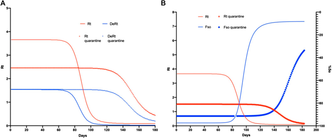
FIGURE 7. SIR1 model comparing regular parameters with quarantine. In (A) the simulation of Rt is observed in the SIR1 model varying the parameters with and without quarantine throughout the epidemic duration. (B) shows the number of infections without quarantine (blue) and with quarantine (red).

Upon application of all the different data of R0, an issue was observed when an immunization appeared (even for vaccination or herd immunity). The most important question is how long will it take to observe if this strategy is successful. Our model showed that, without quarantine from day-80 to day 100, the introduction of vaccination, the rebound of immunized individuals, and a decrease in the number of infected cases applying quarantine between day 100 to day 120 would result in the same outcome (Figure 8).

FIGURE 8

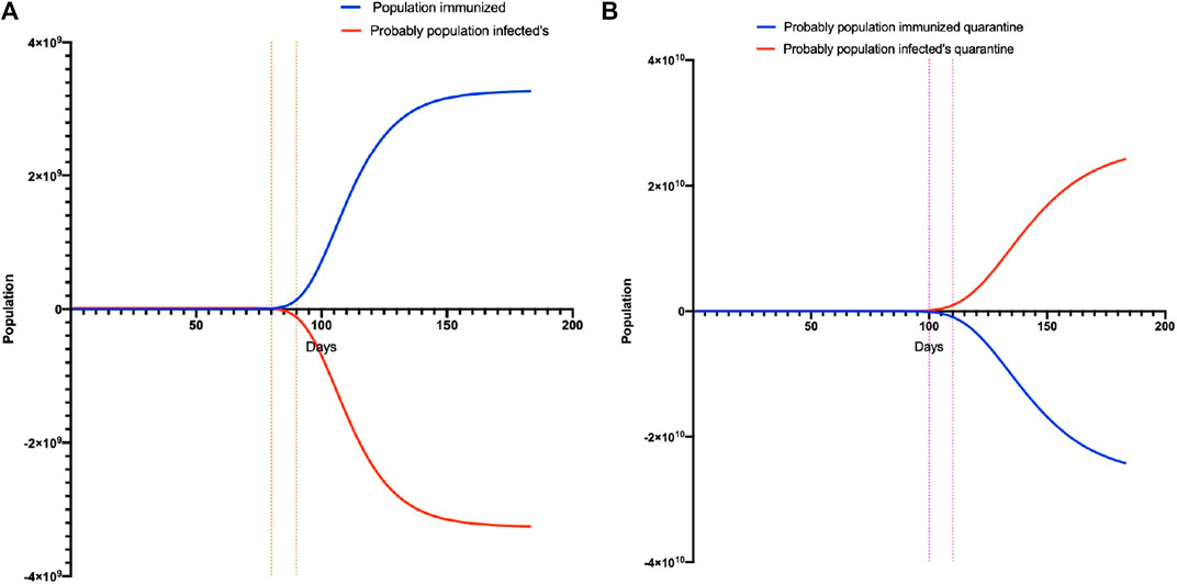
FIGURE 8. Calculation model to reach herd immunity. (A) is the model without quarantine and shows the time that must pass for herd immunity to occur. (B) is the model with quarantine and shows the time that must pass for herd immunity to occur.

4. Discussion

The model used in our study is not the only model to predict the behavior of COVID-19. One must consider the dynamic of SARS-CoV-2 transmission, availability of resources, and delay in diagnosis when choosing the best model. For Ecuador, an important issue was the large number of people with pending SARS-CoV-2 tests. This factor, together with asymptomatic individuals and underreporting of “true” infected people (by consensus, it is 55%), demonstrated why our model was not well-fitted with the data reported by the MSP [9, 23].

Although the estimated time needed for a patient to recover from COVID-19 was 18–20 days, some scholars have stated it is 8–10 days using SIR models. According to the MSP, it takes 20 days, which poses problems for healthcare units in terms of space and resources [5, 23, 24]. Determining this value is a key component in the prediction based on SIR models because it is based on local data. Subsequently, extrapolations can be made in the hope that they are not too far from reality.

In our study, the time for recovery from COVID-19 was based on a K model and observing how the recovery curve was adjusted to the true situation. Mistakes can be generated because of the issues mentioned above as well as from the reports of patients who have recovered from COVID-19. Even though this value cannot be observed directly, it can be estimated through the report of deaths by the MSP and comparing them with the registry of the National Institute of Statistics of Ecuador. This comparison resulted in a difference of ≥20% and has been observed in other studies too [23–26].

Through an assessment of the first 100 cases of COVID-19, a marked difference in acceleration and control of the epidemic was made in Taiwan. The Taiwan government isolated and quarantined all individuals related to each COVID-19 case, and tracked all asymptomatic individuals. This strategy showed that, according to the proposed model, quarantining the first six cases rapidly and aggressively would have created a different scenario from that seen presently but, as the author mentions, the switch from theory to practice is not easy [25]. Another important observation is the rate of increase of cases. At the national level, the rate of increase was constant (the number of cases increased in 5–7 days), as has been observed on a global scale [9, 27]. Hence, locally obtained data were a reflection of what occurred in the past when SARS-CoV-2 spread in Asia and Europe [9, 27].

Our model estimated that lifting the quarantine should occur approximately 2–3 months after the peak of infection has been reached. In China, after the peak of infection (after 17 days), the quarantine was lifted during day 13 to day 14. Such lifting is dependent upon time and the capacity of the health system of a particular country. In addition, a strict quarantine works not only by holding back the appearance of new cases, but also allows the health system to recover and prepare for new cases [5, 27].

The mortality rate for COVID-19 has been estimated to be about 3–7%, and results in another problem for SIR models. In our model, we took a mortality rate of 5% (in other models, it varies between 3 and 4.5%). However, one must consider other causes of death unrelated to COVID-19 that can affect a model indirectly [5, 23, 24, 29]. The increase in R0 determines how effective the strategies taken by local authorities are. In our study, R0 = 2.2, which is not too far from the international trend (Ye et al. estimated the same value of R0, and the World Health Organization value is between 1.4 and 2.5).

The time of infection is generated based on R0 (which depends on whether the value increases or decreases). If we compare the R0 for other diseases caused by viruses of the same family (Middle East respiratory syndrome-related coronavirus, <1; SARS, 2–4), this value does not reflect the lethality for each one [5, 23, 27, 30, 31]. Hence, defining R0 is not easy and is mired in controversy. Each population could “fix” their value and reflect the variation in parameters of the equation used (β and α) in each SIR model. The latter could be constructed and calculated in different ways depending on data reliability. However, the R0 is very important because from it the minimum number of immunized people required to stop the epidemic, and the maximum number of individuals susceptible to infection, can be calculated [10, 11, 32, 33].

Some problems were identified when the R0 was calculated on the basis of the total population. However, in reality, interventions are applied only in specific or priority groups. We analyzed different R0 values for the COVID-19 epidemic in Ecuador and, despite an increase in R0, 100% of a population will not be infected. With the prediction models used for smallpox prevention, the R0 was 10, but the maximum percentage of infected individuals in a vulnerable population was 70% and, upon introduction of a vaccine, any epidemic can be prevented with a coverage of 60% of the population [6, 16].

Complex and dynamic clinical phenomena occur during disease development. The immune response, nutritional state, chronic diseases, or co-infections can interfere (accelerate or decelerate) epidemic expansion, and are not taken into account when the R0 is calculated [11]. Hence, Li and colleagues [11] postulated the interpretation and analyses of R0 in four categories. Their model explains the rapid expansion of a disease but with a relatively slow recovery process.

Rt provides a clearer picture of the time of increase of an epidemic according to the percentage of susceptible people over time. Initially, the Rt shows an acceleration in the number of infected individuals, then becomes constant at the end of the epidemic, and reaches a value of 0, thereby allowing calculation of an adjusted R0 adapted to constant changes or population variation over time [33, 34]. A bottleneck has been observed in the Rt as the number of days of an epidemic increase, and the R0 is closer to reality because, with fewer people to infect, the true infective capacity of a virus is observed. However, this scenario was not entirely accurate in our model (R0 = 1.97). Even though our R0 is lower than that reported worldwide, some scholars have calculated an R0 value between 0 and 1. This does not mean that an epidemic is improving or ending; in some cases, this value shows a latency period [11, 32, 34, 35]. For a more accurate adjustment of the R0, we applied Fso based on our obtained Rt value. As seen in Figure 7, the point where both curves intersect corresponds to the R0 and simultaneously coincides with the bottleneck observed in Rt (Figure 5), and we showed a similar value of R0 to that obtained in previous studies [10, 33].

The minimum number of infected people required to stop an epidemic has been mentioned [9, 23, 33, 36]. However, this value must be considered very carefully because these infected individuals will probably die. Importantly, 60% of the population should be immunized (based on R0) to stop the COVID-19 epidemic in Ecuador [9, 23, 33, 36]. This concept is seen more clearly with “collective immunity” or “collective protection”, which refers to the fact that a group of infected people who recover will prevent the disease from spreading to the entire population [21, 22, 37]. By applying this concept to our SIR models, this collective protection will be reached with 60% of the infected population but, as stated by Rashid and colleagues, there are three main problems of assuming this value as real.

The first problem is the heterogeneity of the population (i.e., the different immune responses that each person presents to SARS-CoV-2). Hence, even though 60% of the population can be infected, this does not ensure that people can generate an immune state that protects the remaining susceptible members of the population [35, 37].

The second problem refers to the R0 and the criterion of the equation for %Pi,v. Rashid et al. explained that, because the population is composed mostly of people at a high risk of contagion, the R0 is overestimated. Hence, collective protection does not correspond to the one that has been calculated. In these cases, one must include in the equation the efficiency of the country’s vaccination campaigns to understand how the epidemic can be controlled [20, 35, 37]. This was not applied in the present study because a vaccine for COVID-19 has not yet been found.

The third problem identified by Rashid et al. is the possible impact of co-circulation of other pathogens (depends on the characteristics of each population) during an epidemic. This could modified SIR models through the calculated R0 with less or more impact in predictions, and not are fitted to reality.

We evaluated the impact of the quarantine implemented in Ecuador using two variables: the percentage of people quarantined (used in the SIR model) and Rt variation (by the effect of this measure). Quarantine reduces the number of people on the streets, and decreases the number of SARS-CoV-2 infections in a particular period [23, 24]. We took as a reference the percentage of people quarantined as 40%. Other models have considered 10%, and observed a decrease of 50% in the number of expected cases that would be observed if no health strategy was implemented. This 50% reduction does not mean that the cases will not exist, only that they will be redistributed over the duration of the epidemic. Hence, the epidemic would last 300 days due to the quarantine instead of 180–200 days, thereby ensuring that the health system does not collapse [29, 30]. Although quarantine has been a good strategy for control of infectious diseases, it is not considered a good strategy from dynamic and economic viewpoints because external factors will affect Fso (the maximum number of susceptible people that can be infected). In our model, Fso increased by 10% (from 80 to 90%) if quarantine was applied in 40% of the population. This increase occurred because the longer the quarantine lasts, the greater the probability that the population will not comply with it. Since quarantine was applied in Ecuador, the unemployment rate increased from 3.9 (2019) to 4.4% (2020). This increase forced people to take to the streets in search of work and increased the number of people exposed to SARS-CoV-2, and, consequently, Fso increased [24, 34, 38].

We also estimated the number of people with acquired immunity to SARS-CoV-2 based on the R0. We showed that a decrease in the number of newly infected cases would be observed by day 80 to day 100 of the epidemic. Other scholars say that this value depends on the responsiveness of the local government to report and identify cases, diagnostic capacity, and the delay in sample processing [9, 23, 33, 36].

We identified a delay in sample processing in ≥40% of cases, this parameter has not been reported before. Another value that can be estimated through the R0 and Fso is the duration of infection. If 40% of the population were in quarantine, we estimated that the duration of infection would increase to 15 days, which was also observed by Li et al. and Massed et al. Both research teams agreed that the duration of infection and number of immunized individuals should not be taken into account to estimate the reduction of an epidemic. A latency period denotes the time when reinfections occur or the epidemic disappears. Hence, if we know the R0, we could estimate the percentage of infected people required to stop the epidemic, which is equivalent to the one during this latent period. Our model determined it to be 65% but, in reality, this value will not be observed until it reaches 90% of infected people and only then will we observe a decrease in the infection rate [11, 23, 24, 33].

Although SIR models provide accurate data for the number of patients who have recovered from COVID-19, infected cases, and exposed patients, they require a large volume of reliable data. SIR models could be used in countries with better contingencies and strategies than those in most Latin American countries. Traditional models are dimensionless in time (results are not affected whether days or months are used) so the infection rate will not fit well with dynamic populations. For our models, we used a specific unit of time that allowed for the daily adjustment and discreet visualization of an increase or decrease of the epidemic. In the context of public health, the use of our model could enable prompt redistribution of resources according to infection trends.

A weakness of our models was not providing the percentage of asymptomatic cases and exposed cases. This led to a reduction of the power of prediction for infected people (≥15%). Although this percentage could affect the fit between the real curve and model curve, this range of variation is acceptable because the exact proportion of asymptomatic COVID-19 individuals in Ecuador is not known. A lack of reliable and updated data was the main limitation of our models. This resulted from a deficiency in the structure of surveillance measurements taken, identification of cases, sample-processing capacity, as well as weakness in recollection, updating, and data analyses from the MSP during the COVID-19 epidemic. The MSP is the only entity that possesses full access to the data, and those data are not open for external analyses or validation. In addition, the number of reported cases and tests performed changed dramatically over time without robust justification from the MSP. Another important limitation was the assumption of some of the parameters for our models. They were obtained from countries from the same region with similar behavior of SARS-CoV-2 infection/COVID19 so did not affect our results.

5. Conclusions

For the entire Ecuadorian population, we estimated that R0 = 2.2, with 88% susceptible/infected individuals. To stop a national epidemic, a quarantine for 3–4 months is required, and when 55% of the population has been immunized (equivalent to 110 days since the first report of a COVID-19 case), a real decrease of new cases will be observed. The effectiveness of quarantine should be analyzed retrospectively, and not as a result of contemporary control of the COVID-19 epidemic.

Data Availability Statement

The raw data supporting the conclusions of this article will be made available by the authors, without undue reservation.

Author Contributions

PE and ET conceptualize the study, PE and PQ obtained data and analyzed it, PE set up the mathematical models, PE and PQ run the models, ET reviewed results and provided feedback. PE and PQ drafted the manuscript. ET drafted the final version. All authors revised and approved final version.

Conflict of Interest

The authors declare that the research was conducted in the absence of any commercial or financial relationships that could be construed as a potential conflict of interest.

References

1. Anthony, SJ, Johnson, CK, Greig, DJ, Kramer, S, Che, X, Wells, H, et al. Global patterns in coronavirus diversity. Virus Evolut (2017). 3(1):1–15. .

PubMed Abstract | CrossRef Full Text | Google Scholar

2. Lal, SK. Molecular biology of the SARS-coronavirus. In: SK, Lal, editor Climate change 2013—the physical science basis. Vol. 53. Cambridge, United Kingdom: Cambridge University Press (2010). p. 1–30). doi:10.1017/CBO9781107415324.004

CrossRef Full Text | Google Scholar

3. Miller, SL, Gill, J, and Webb, GR. The proximal origin of the hamstrings and surrounding anatomy encountered during repair. J Bone Joint Surg (2007). 89(1):44–8. doi:10.2106/jbjs.f.00094.

PubMed Abstract | CrossRef Full Text | Google Scholar

4. Jin, Y, Yang, H, Ji, W, Wu, W, Chen, S, Zhang, W, et al. Virology, epidemiology, pathogenesis, and control of covid-19. Viruses (2020). 12(4):1–17. doi:10.3390/v12040372.

CrossRef Full Text | Google Scholar

5. Ye, Q, Wang, B, Mao, J, Fu, J, Shang, S, and Shu, Q. Epidemiological analysis of COVID-19 and practical experience from China. J Med Virol (2020). 12:23–7. doi:10.1002/jmv.25813

CrossRef Full Text | Google Scholar

6. Kaul, D. An overview of coronaviruses including the SARS-2 coronavirus—molecular biology, epidemiology and clinical implications. Curr Med Res Pract (2020). 10(2):54–64. doi:10.1016/j.cmrp.2020.04.001.

CrossRef Full Text | Google Scholar

7. Rothan, HA, and Byrareddy, SN. The epidemiology and pathogenesis of coronavirus disease (COVID-19) outbreak. J Autoimmun (2020). 109, 102433. doi:10.1016/j.jaut.2020.102433.

PubMed Abstract | CrossRef Full Text | Google Scholar

8.SNGRE, CIES. Covid-19 en el ecuador tendencia temporo espacial de la pandemia del 27 de febrero al 19 de abril del 2020 INFORME. New York City, NY: MINTEL (2020).

Google Scholar

9.MSP. Informes de Situación e Infografias—COVID 19—desde el 29 de Febrero del 2020—Servicio Nacional de Gestión de Riesgos y Emergencias. Quito, Ecuador: Ministerio de Salud Pública (2020).

Google Scholar

10. Bjornstad, ON. Epidemics models and data using R. Berlin, Germany: Springer (2010). doi:10.1007/978-3-319-97487-3

CrossRef Full Text | Google Scholar

11. Li, J, Blakeley, D, and Smith, RJ. The failure of R0. Comput Math Methods Med (2011). 2011:1–17. doi:10.1155/2011/527610

CrossRef Full Text | Google Scholar

12. Vynnycky, E, and White, R. An introduction to infectious disease modelling. Oxford, UK: Oxford University Press (2010).

Google Scholar

13. Keeling, MJ, and Rohani, P. Modeling infectious diseases through Contact networks. Princeton, NJ: Princeton University Press (2008).

Google Scholar

14. Li, MY. An introduction to mathematical modeling of infectious diseases. In: Ken, L, and Golden, M editors. An introduction to mathematical modeling of infectious diseases. 2nd ed. Berlin, Germany: Springer International Publishing (2018). doi:10.1007/978-3-319-72122-4

CrossRef Full Text | Google Scholar

15.NHCPRC. Latest developments in epidemic control. National Health Commission of the People’s Republic of China (2020).

Google Scholar

16. Jones, JH. Notes on R 0. Building (2011). 1–19:17–33. doi:10.1186/isrctn10820810

CrossRef Full Text | Google Scholar

17. Kretzschmar, M. Measurement and modeling: infectious disease modeling. In: International encyclopedia of public health. 2nd ed. Vol. 4. Amsterdam, Netherlands: Elsevier. doi:10.1016/B978-0-12-803678-5.00229-0

CrossRef Full Text | Google Scholar

18. Tarigan, PB. Veterinary epidemiology. J Chem Inf Model (2013). 53(9):58–67. doi:10.1017/CBO9781107415324.004

CrossRef Full Text | Google Scholar

19. Balkew, TM. The SIR model when S(t) is A multi-exponential function. East Tennessee State University (2010). 12 p.

Google Scholar

20. Smith, DR. Herd immunity. Vet Clin North Am Food Anim Pract (2019). 35(3):593–604. doi:10.1016/j.cvfa.2019.07.001.

PubMed Abstract | CrossRef Full Text | Google Scholar

21. Chen, J, Ye, L, Zhou, MY, Cheng, YR, Wang, M-W, and Feng, ZH. Herd immunity and COVID-19. Eur Rev Med Pharmacol Sci (2020). 24(8):4064–5. doi:10.26355/eurrev_202004_20978.

PubMed Abstract | CrossRef Full Text | Google Scholar

22. Kwok, KO, Lai, F, Wei, WI, Wong, SYS, and Tang, JWT. Herd immunity—estimating the level required to halt the COVID-19 epidemics in affected countries. J Infect (2020). 80(6):e32–3. doi:10.1016/j.jinf.2020.03.027.

PubMed Abstract | CrossRef Full Text | Google Scholar

23. Castro, P, De los, R, Juan, C, González, S, Merino, P, and Ponce, J. Modelización y simulación de la propagación del virus sars-cov-2 en Ecuador. MODEMAT (2020). Available from: https://observatoriocovid19.sv/doc/biblioteca/internac/Informe-Covid19-Modemat.pdf.

Google Scholar

24. Aguirre, H, Orellana, D, and Armas, R. Escenarios de Propagación de COVID-19 al 21 de Abril y Relajamiento de Medidas de Mitigación. Cuenca, Ecuador: Universidad de Cuenca (2020). p. 1–14.

Google Scholar

25. Cheng, H-Y, Jian, S-W, Liu, D-P, Ng, T-C, Huang, W-T, and Lin, H-H. Contact tracing assessment of COVID-19 transmission dynamics in Taiwan and risk at different exposure periods before and after symptom onset. JAMA Intern Med (2020). 180:1156–63. doi:10.1001/jamainternmed.2020.2020.

PubMed Abstract | CrossRef Full Text | Google Scholar

26.INEC. Estadísticas Vitales registro estadístico de Nacidos vivos y Defunciones 2016. INEC (2016). 1, 315. doi:10.1016/j.jhazmat.2015.06.018

CrossRef Full Text | Google Scholar

27. Bulut, C, and Kato, Y. Epidemiology of COVID-19. Turk J Med Sci (2020). 50(SI-1), 563–70. doi:10.3906/sag-2004-172.

PubMed Abstract | CrossRef Full Text | Google Scholar

28. Petrosillo, N, Viceconte, G, Ergonul, O, Ippolito, G, and Petersen, E. COVID-19, SARS and MERS: are they closely related? Clin Microbiol Infect (2020). 22:74–8. doi:10.1016/j.cmi.2020.03.026

CrossRef Full Text | Google Scholar

29. Stratton, SJ. COVID-19: not a simple public health emergency. Prehosp Disaster Med (2020). 35(2):119. doi:10.1017/s1049023x2000031x.

PubMed Abstract | CrossRef Full Text | Google Scholar

30. Panovska-Griffiths, J. Can mathematical modelling solve the current Covid-19 crisis? BMC Publ Health (2020). 20(1):1–3. doi:10.1186/s12889-020-08671-z.

CrossRef Full Text | Google Scholar

31. Uras, U. Coronavirus: comparing COVID-19, SARS and MERS|news|Al Jazeera (2020). Available from: https://www.aljazeera.com/news/2020/04/coronavirus-comparing-covid-19-sars-mers-200406165555715.html

Google Scholar

32. Breban, R, Vardavas, R, and Blower, S. Theory versus data: how to calculate R0? PLoS One (2007). 2(3):e282. doi:10.1371/journal.pone.0000282.

PubMed Abstract | CrossRef Full Text | Google Scholar

33. Massad, E. Ethical and Transborder issues. Global Health Inform (2017). 12:232–63. doi:10.1016/B978-0-12-804591-6.00012-4

CrossRef Full Text | Google Scholar

34. Akpan, N. How to measure your nation’s response to coronavirus. London, UK: National Geographic (2020).

Google Scholar

35. Metcalf, CJE, Ferrari, M, Graham, AL, and Grenfell, BT. Understanding herd immunity. Trends Immunol (2015). 36(12):753–55. doi:10.1016/j.it.2015.10.004.

PubMed Abstract | CrossRef Full Text | Google Scholar

36. Sun, K, Chen, J, and Viboud, C. Early epidemiological analysis of the coronavirus disease 2019 outbreak based on crowdsourced data: a population-level observational study. Lancet Dig Health (2020). 2:e201–8. doi:10.1016/S2589-7500(20)30026-1

CrossRef Full Text | Google Scholar

37. Rashid, H, Khandaker, G, and Booy, R. Vaccination and herd immunity. Curr Opin Infect Dis (2012). 25(3):243–9. doi:10.1097/qco.0b013e328352f727

PubMed Abstract | Google Scholar

38. Lombeida, E, Moreno, L, and Fabara, C. Pobreza y desigualdad Ecuador (2010). Available from: http://www.ecuadorencifras.gob.ec/documentos/web-inec/POBREZA/2018/Junio-2018/Informe_pobreza_y_desigualdad-junio_2018.pdf

Google Scholar