Understanding Deep Learning: Expected Spanning Dimension and Controlling the Flexibility of Neural Networks

1 Introduction

Neural networks (NN) have wide applications in machine learning [1]. For example, in the field of computer vision, convolutional NNs, a specific type of feed-forward NN, greatly outperform any previous traditional computer vision method [2]. However, there are many questions that arise when analyzing large-scale NNs. A deeper theoretical understanding of NNs, besides being a useful goal in itself, can often lead to improved performance on practical real-world problems. In this article, we develop a method to measure the flexibility of an NN, independent of any input data, that is both easily computed and is highly correlated with the testing accuracy of the NNs on standard benchmark datasets. We accomplish this by considering a basis of functions to represent the NN and then analyzing the dimension of the range of the function of the inputs of the NN to the coefficients of the output of the NN with respect to that basis. In particular, our perspective is inspired by classic results in analysis, such as Sard’s theorem [3] and the Reisz representation theorem. Analyzing the rank of appropriately defined Jacobians, which arise naturally from NNs, is one of our key analytical tools. Such Jacobians can be efficiently computed using the automatic differentiation capabilities of deep learning libraries like PyTorch and TensorFlow. We demonstrate how thinking about NNs from such a perspective leads naturally to NNs with improved performance.

NNs are quite popular in many applied problems. The understanding of their performance is often measured in relation to training data and specific learning algorithms [4, 5]. However, NNs often exhibit surprising properties which seem to be at odds with other classic machine learning techniques. For example, in [6], the authors provide strong evidence that understanding the performance of NNs will likely require a rethinking of generalization and the role that the number of parameters of a given machine learning algorithm play in its ability to generalize to new data. Analyzing NNs from the perspective of their generalization performance has led to several important research directions including recent work in “double descent” analysis [7–9], the use of the Takeuchi information criterion [10], the statistical capacity of NNs [11], Kolmogorov Width decay [12], and even analyzing NN capacity from the point of view of algebraic topology [13]. The idea of “double descent” [7–9] begins with the classic bias–variance trade-off curve, where the testing error of a given learning system is small for moderately flexible algorithms but large for under flexible or over flexible algorithms. It then proceeds to observe that as algorithm flexibility increases even further, for certain classes of algorithms, a point is reached at which increasing flexibility begins to again improve testing accuracy (this is the second of the “double descents”). In another direction of research, the Takeuchi information criterion [10], classic extension of the Akaike information criterion (AIC), is used to study NNs. Other similar approaches have developed newer estimators including considering flatness of minima [14] and measures of NN sensitivity to their inputs [15]. The authors of [11] take a wide view of such matters, and make connections among measures of NN performance such as sharpness, robustness, and norm-based control, and PAC-Bayes theory. In [12], the authors study Kolmogorov Width decay in the context of NNs, and they prove several interesting results, including showing that wide NNs can be susceptible to the curse of dimensionality, while shallow NNs are not. While such methods have been widely used in domains such as studying the properties of PDEs, such an approach would seem to have computational hurdles to overcome when applied to large-scale NNs. We also observe that many interesting directions are possible for studying NNs, and even ideas such as algebraic topology have an important role to play [13]. In addition, a recent (2020) survey of NN architectures, including discussion of their representation capacities, can be found in [16]. Our work can be viewed as complementary to ideas such as those in [10, 11], but instead approaching the problem of evaluating NNs from a more analytic point of view.

In particular, our work differs from this body of work in a number of ways. First, the main computational effort required by our analysis is a natural by-product of the classic backpropagation procedure widely used in the optimization of NNs. We can leverage already existing and highly optimized routines for constructing the Jacobians that we require, and our analysis can be accomplished with a cost that is roughly the same as that required by a few hundred backpropagation steps. Second, our analysis applies to NNs ranging from the smallest NNs of which we can conceive to large-scale real-world networks used for practical tasks such as image understanding. Third, and perhaps most importantly, our proposed ESD metric is highly correlated with the generalization performance on both small NNs, in which all details can be theoretically justified, and large real-world networks. As we will demonstrate, considering ESD provides insights into the performance of NNs and provides suggestions on how this performance can be improved.

2 Background

2.1 A Simple Example to Inspire the Approach

Consider the simple multilayer perceptron $N_{\theta }$ with one input, one output, two hidden layers, each with one node, and activation functions $f\left(z\right)=z^2$. While quite simple, this function embraces two key aspects of NNs. In particular, it is a composition of simple affine transformations, as is classic for layers of an NN, but is not itself an affine function because of the nonlinear activation function.

This simple NN can be written as

$N_{\theta }\left(x\right)=w_3{(w_2{(w_{1}x+b_1)}^2+b_2)}^2+b_3,(1)$

where $w=\left\{w_1,w_2,w_3\right\}$ are the scalar weights of the NN, $b=\{b_1,b_2,b_3\}$ are the corresponding scalar biases, and $\theta =w\cup b$. Note that for our particular simple choice of activation functions, Eq. 1 is a 4th degree polynomial in x with six free parameters. We can expand this polynomial to obtain the coefficients of the basis $1,x,x^2,x^3,\dots$

$\begin{array}{c}{N}_{\theta }\left(x\right)=\left(w_1^4{w}_2^2{w}_3\right)x^4\\ +\left(4b_1{w}_1^3{w}_2^2{w}_3\right)x^3\\ +\left(6b_1^2{w}_1^2{w}_2^2{w}_3+2b_2{w}_1^2{w}_2{w}_3\right)x^2\\ +\left(4b_1^3{w}_1{w}_2^2{w}_3+4b_1{b}_2{w}_1{w}_2{w}_3\right)x\\ +(b_1^4{w}_2^2{w}_3+2b_1^2{b}_2{w}_2{w}_3+b_2^2{w}_3+b_3)\\ ={\left[\begin{array}{c}{x}^4\\ x^3\\ x^2\\ x\\ 1\end{array}\right]}^T\left[\begin{array}{c}\left(w_1^4{w}_2^2{w}_3\right)\\ \left(4b_1{w}_1^3{w}_2^2{w}_3\right)\\ \left(6b_1^2{w}_1^2{w}_2^2{w}_3+2b_2{w}_1^2{w}_2{w}_3\right)\\ \left(4b_1^3{w}_1{w}_2^2{w}_3+4b_1{b}_2{w}_1{w}_2{w}_3\right)\\ \left(b_1^4{w}_2^2{w}_3+2b_1^2{b}_2{w}_2{w}_3+b_2^2{w}_3+b_3\right)\end{array}\right]\\ =P{\left(w,b\right)}^T\text{Φ}\left(x\right)\end{array}(2)$

for our set of polynomial basis functions $\Phi \left(x\right)=1,x,x^2,x^3,\dots$, and a parameterized set of weights for these basis functions encoded in $P(w,b)$. A critical idea that will be discussed in detail is that this representation $N_{\theta }\left(x\right)=P{\left(w,b\right)}^T\text{Φ}\left(x\right)$ is not unique. The Reisz representation theorem [3] shows that we could have selected another basis for $\theta \left(x\right)$ such as Legendre polynomials or Fourier basis functions. However, for this example, the standard polynomial basis is the most natural setting and allows us to represent the NN with a finite number of coefficients. As we generalize our analysis to nonpolynomial NNs, we will consider other bases.

One can then compare 2 to the standard polynomial form with five weights

$p\left(x\right)=a{x}^4+b{x}^3+c{x}^2+dx+e(3)$

and consider whether the set of functions that 2 and 3 can represent, given arbitrary weights, are equivalent. It is clear that 3 can represent all 4th-order polynomials, but 2 is rather more complicated. One might ask what set of 4th-order polynomials 2 can represent.

Similar to the line of thought in [18] for linear models, one can approach 2 and 3 as different parameterizations of the space of all 4th degree polynomials. In particular, when comparing 2 and 3, it might seem reasonable, at first glance, to guess that the six parameters of 2 would allow it to have the same representation power as 3, since the latter has only five parameters. However, this is not the case. In fact, the set of all polynomials of degree 4 that $N_{\theta }\left(x\right)$ can represent is of measure 0 in the space of all 4th degree polynomials. The function $N_{\theta }\left(x\right)$ is less expressive than 3 due to the way the weights are shared among the coefficients of the polynomial. We note that this coefficient sharing between terms of the polynomial expansion of the simple NNs $N_{\theta }\left(x\right)$ is not a special aspect of $N_{\theta }\left(x\right)$ but rather a property of the fact that $N_{\theta }\left(x\right)$ is written using a combination of function composition and nonlinear activation functions, both of which are essential properties of NNs.

To measure just how restricted the polynomial form of $N_{\theta }\left(x\right)$ is, we consider the function $P\left(w,b\right):{\mathrm{ℝ}}^6\to {\mathrm{ℝ}}^5$ that maps the 6 parameters (weights and biases) to the five coefficients of the polynomial basis $\text{Φ}\left(x\right)$. While the domain of $P\left(w,b\right)$ encompasses all of ${\mathrm{ℝ}}^6$, since each parameter can be any real number, the range of this function does not fill all of ${\mathrm{ℝ}}^5$. In fact, as we will compute below, the dimension of the range of is 4.

We can compute this dimension of the range of $P\left(w,b\right)$ by considering the rank of its Jacobian. By Sard’s theorem [3], this rank is constant everywhere, except for a set of measure 0. If we substitute (nonzero) random values for the 6 parameters and compute the rank of the resulting matrix; with probability 1, the result will be the dimension of the range of $P\left(w,b\right)$. For example, choosing arbitrary values $w_1=3$, $w_2=9$, $w_3=7$, $b_1=2$, $b_2=-4$, and $b_3=-6$, we obtain,

$J_c=\left[\begin{array}{cccccc}\mathrm{61,236}& \mathrm{10,206}& 6561& 0& 0& 0\\ \mathrm{122,472}& \mathrm{27,216}& \mathrm{17,496}& \mathrm{61,236}& 0& 0\\ \mathrm{78,624}& \mathrm{26,712}& \mathrm{16,848}& \mathrm{122,472}& 1134& 0\\ \mathrm{16,128}& \mathrm{11,424}& 6912& \mathrm{78,624}& 1512& 0\\ 0& 1792& 1024& \mathrm{16,128}& 448& 1\end{array}\right].(4)$

Here, we used integers so that we can compute the exact rank without taking into account any floating point uncertainties. Using standard symbolic manipulation software [19], the rank of this matrix can be computed analytically without appealing to any numerical approximations. The rank of this matrix is 4. Again, as 2 is analytic function, we may apply Sard’s theorem [3] to show that the rank is constant everywhere except for a set of measure 0. As a numerical exercise, we computed the rank of the Jacobian at thousands of other random input weights, and, unsurprisingly, we consistently obtained a rank of 4.

The foundational idea is that, while the simple polynomial NN, $N_{\theta }$ appears to have 6 degrees of freedom and be a multiple covering of the space of all polynomials; it actually only has 4 degrees of freedom, and the representation power of the NN is smaller than expected. However, this does not tell us which polynomials are accessible to the NN. At first glance, one might assume that having 4 parameters means that only 3rd degree polynomials are representable, since representing all 3rd degree polynomials required 4 parameters. However, there are polynomials of degree 4 which are clearly expressible by the network, just not all 4-th degree polynomials. For example, take $w_1=w_2=w_3=1$ and set the rest of the parameters equal to any arbitrary values. Accordingly, the polynomial representation $N_{\theta }\left(x\right)$ should not be thought of necessarily penalizing higher-order polynomials, but rather selecting a subset of polynomials that includes both high and low-order polynomial representatives. This somewhat odd behavior arises from the fact that the 4th order polynomials in question are represented by way of function composition, which is one of the defining characteristics of deep NNs.

2.2 Definition of Polynomial Spanning Dimension

Inspired by the simple NN in 2, we now define the following.

Definition 1. Given a polynomial NN of the form $N_{\theta }\left(x\right)=\text{Φ}{\left(x\right)}^{T}P\left(\theta \right)$ with $P:{\mathrm{ℝ}}^m\to {\mathrm{ℝ}}^k$ and $\text{Φ}:\mathrm{ℝ}\to {\mathrm{ℝ}}^k$, where m is the number of trainable weights, k is one more than the degree of the polynomial, and $\Phi \left(x\right)=1,x,x^2,x^3,\dots$, we define the polynomial spanning dimension (PSD) of $N_{\theta }\left(x\right)$ as the maximal rank of the Jacobian matrix of $\frac{\partial P\left(\theta \right)}{\partial \theta }$ over all θ and x.From a theoretical point of view, Definition 1 can have interesting implications. For example, here is one theorem that naturally arises.

Theorem 2.1. Let N be an NN with a single input and output, l hidden layers, and height 1 (a single node per hidden layer) with polynomial activation functions in the hidden layers. Let $D\left(N\right)$ be the PSD of N, then $D\left(N\right)\le l+2$.The proof can be found in the Supplementary Material.One can imagine that many theorems of a similar flavor could easily be posed and proven.

3 Developing a More General Definition of Spanning Dimension

In Definition 1, we made three assumptions about the NN $N_{\theta }\left(x\right)$.

1)   We assume that $N_{\theta }\left(x\right)$ is a polynomial. However, this rarely occurs in practice.

2)   We assumed that the activation functions are smooth. Common activation functions like ReLU [20], though differentiable almost everywhere, are not smooth.

3)   The NN has only one input and output.

In this section, we will address and relax each of these assumptions in turn and generalize our definition of PSD to apply to a much larger class of NNs including those found in real-world applications.

3.1 Generalizing Spanning Dimension to Nonpolynomial Neural Networks

In Definition 1, we are representing a polynomial as the coefficients of the polynomial basis $1,x,x^2,x^3,\dots$. A single function $N_{\theta }\left(x\right)$ may have more than one representation as $\text{Φ}{\left(x\right)}^{T}P\left(\theta \right)$ for different choices of P and $\text{Φ}$. In particular, the existence of the decomposition $N_{\theta }\left(x\right)=\text{Φ}{\left(x\right)}^{T}P\left(\theta \right)$ is a finite dimensional special case of the famed Riesz representation theorem [17], which guarantees, under quite general circumstances, that the infinite dimensional analog of such decompositions always exists for quite general classes of functions. In this section, we will develop a definition of SD that does not depend on the particular representation $\text{Φ}{\left(x\right)}^{T}P\left(\theta \right)$ chosen, but rather on more general properties of NNs themselves.

When we computed the PSD of polynomial NNs, we considered the coefficients of the polynomial in terms of the polynomial basis $1,x,x^2,\dots ,x^n$. With 3, we saw that we could independently adjust each coefficient without affecting the other coefficients. However, with 2, this was not true. Adjusting one coefficient has an impact on the other coefficients. It is precisely this restriction which results in a PSD < 5.

With a polynomial of the form presented in 3, the number of weights is equal to the number of points $x_1,x_2,\dots ,x_n$, $y_1,y_2,\dots ,y_n$ (provided that $x_i\ne x_j$ for $j\ne i$) that one can fit exactly. A necessary condition to be able to fit n arbitrary points is that the range of the function from the weights to the coefficients of the polynomial is of dimension n or greater. It is important to emphasize that this is only a necessary condition and not a sufficient one. Consider the following polynomial,

$\widehat{y}=p\left(x\right)=a^2{x}^2+b^2.(5)$

Clearly, we cannot ever fit $x=1$ and $\widehat{y}=-2$ because $p\left(x\right)\ge 0$ for all $x\in \mathrm{ℝ}$ no matter what the values of the weights a and b happen to be. However, the PSD of this polynomial is still 2.

In the case of polynomials with one input and output, we will now show that an equivalent way to compute the PSD is to determine the rank of the Jacobian of the function from w unique fixed input points to the w output points with respect to the weights of the polynomial, where w is the number of weights in the NN. Note that with this definition, one no longer needs the individual coefficients of the polynomial. One only needs to be able to evaluate the polynomial for a given set of inputs. This is a critical step in generalizing the definition of spanning dimension to nonpolynomial NNs. We will start with a simple example to illustrate the concept.

Consider the NN, $N_{\theta }\left(x\right)$, introduced in the previous section. We select six random input points $x_1=1,x_2=3,x_3=5,x_4=-1,x_5=-3,x_6=-4$ and evaluate the NN at these input points to obtain the six output points $y_i=n\left(x_i,w_1,w_2,w_3,b_1,b_2,b_3\right),i=1\dots 6$. We now consider these input points as fixed and compute the Jacobian of the function from the six weights to these resulting six output points. This Jacobian evaluated at $w_1=3$, $w_2=9$, $w_3=7$, $b_1=2$, $b_2=-4$, and $b_3=-6$ is,

$J_n=\left[\begin{array}{cccccc}\mathrm{278,460}& \mathrm{77,350}& \mathrm{48,841}& \mathrm{278,460}& \mathrm{3,094}& 1\\ \mathrm{9,022,860}& \mathrm{1,837,990}& \mathrm{1,177,225}& \mathrm{3,007,620}& \mathrm{15,190}& 1\\ \mathrm{55,627,740}& \mathrm{10,507,462}& \mathrm{6,744,409}& \mathrm{11,125,548}& \mathrm{36,358}& 1\\ \mathrm{1,260}& 70& 25& -\mathrm{1,260}& 70& 1\\ \mathrm{2,312,604}& \mathrm{299,782}& \mathrm{190,969}& -\mathrm{770,868}& \mathrm{6,118}& 1\\ \mathrm{9,031,680}& \mathrm{1,254,400}& \mathrm{802,816}& -\mathrm{2,257,920}& \mathrm{12,544}& 1\end{array}\right].(6)$

This Jacobian has rank 4. We can see that in this specific instance that $J_n$ has the same rank as $J_c$, which was computed in Section 2.1.

We will now show that these two definitions are equivalent for all polynomial NNs. Given a polynomial NN, we have the following relationship,

$J_n=V{J}_c,(7)$

where $J_n$ is the Jacobian of the neural network with respect to the weights as computed in 6, $J_c$ is the Jacobian obtained from computing the derivative of each coefficient of the polynomial with respect to each weight as in 4, and V is the (re-ordered) Vandermonde matrix arising from our choice of polynomial basis [21]. One can see this by noting that $N\left(x,w\right)=VC\left(w\right)$, where $N\left(x,w\right)$ is the polynomial neural network evaluated at the input points, x, w are the weights of the neural network, and $C\left(w\right)$ are the coefficients of the neural network in terms of the standard polynomial basis. Taking the Jacobian of both sides with respect to the weights gives us 7.

Why does computing the rank of $J_n$ allow us to compute the rank of $J_c$? One merely needs to note that when $x_i\ne 0$, $x_i\ne x_j$ for $i\ne j$, we have that V is full rank [21]. Thus, $J_n$ is the same as the rank of $J_c$.

Harkening back to 2, we see that V can be interpreted as our basis functions $\text{Φ}\left(x\right)$ evaluated at our training data $x_1,x_2,\dots ,x_n$ and that $J_c$ can be interpreted as the Jacobian $\frac{\partial P\left(\theta \right)}{\partial \theta }$. However, using the above procedure, the rank of $J_c$ and hence the value of PSD as in Definition 1, can be computed without actually knowing the decomposition$P{\left(\theta \right)}^T\text{Φ}\left(x\right)$of$N_{\theta }\left(x\right)$. This is the key benefit of our approach. In particular, given the above method,

(1) computing $J_n$ can be easily and efficiently achieved for NNs using libraries like PyTorch [22], and

(2) we have a natural extension for the definition of PSD, which we will simply call the spanning dimension (SD) to nonpolynomial NNs since we do not need to actually pick a basis representation of our NN. Rather, this definition is based on the dimension of the range of the function from the NN evaluated at our selected input points to its outputs and is a necessary, but not sufficient, condition for being able to fit those selected input points to arbitrary output points exactly.

3.1.1 Effective Rank

Our second assumption above was that the NN in consideration had smooth activation functions, but that is not the case for real-world NNs which use activation functions like ReLU [20], which are differentiable almost everywhere but are not smooth. In particular, while the ReLU function is piecewise linear, and therefore has a Taylor expansion with only two non-zero terms away from its singularity (as is not defined at the singularity), in the context of the effective rank, we suggest that it is appropriate to think of the ReLU in two ways, which we will explore numerically in Sections 3.1, 5, and 6.

First, as giving rise to a “faceted manifold” where the Jacobian of interest is also piecewise constant, we observe that if the NN is evaluated exactly at a point at which activation is nonsmooth, then the Jacobian of interest will not uniquely be defined there. However, for all standard activation functions, such as ReLU, the set of nonsmooth points for that activation function is of measure-0, so the Jacobian we require is defined uniquely almost everywhere.

Second, as the ReLU being thought of as the limit of a SoftPlus (i.e., smoothed ReLu) [23] type activation, we conjecture that the difference between the ReLu-type activation functions and sigmoid-type activation functions is the leading order coefficients in their Taylor expansions. In particular, while the first nonconstant term for the sigmoid activation function is linear, the first nonconstant term for the SoftPlus is quadratic.

Furthermore, with polynomial NNs, we selected integer inputs to create a Jacobian that consisted of integer entries. For nonpolynomial NNs with many commonly used activation functions, this is not possible. For example, the sigmoid activation function contains an exponential which is irrational. To estimate the rank of a matrix with floating point entries, and thereby the SD, we can consider the singular values of that matrix. One classic method to compute the rank of a matrix from its singular values is to simply count the number of singular values that are greater than a certain tolerance based on machine epsilon. Of course, there are more sophisticated approaches, and one that we use here is the idea of the effective rank and defined in [24].

Let the n singular values of the Jacobian be ${\sigma }_1,{\sigma }_2,\dots ,{\sigma }_n$ and let

$p_i=\frac{{\sigma }_i}{\mathrm{\Vert }\sigma {\mathrm{\Vert }}_1},(8)$

where

$\mathrm{\Vert }\sigma {\mathrm{\Vert }}_1={\displaystyle \sum _{i=1}^n|}{\sigma }_i|.(9)$

The effective rank of the Jacobian is then

$erank\left(J\right)=e^{-{{{\displaystyle \sum }}^{\text{}}}_{i=1}^n{p}_i\log \left(p_i\right)}.(10)$

This approach has a number of important mathematical properties that make it suitable for our analysis. The following three properties are particularly relevant. For a matrix A, and $c\ne 0$, we have,

(1) $1\le erank\left(A\right)\le rank\left(A\right)$, where $rank\left(A\right)$ is the number of nonzero singular values of A.

(2) $erank\left(A\right)=erank\left(A^T\right)=erank\left(cA\right)$.

(3) A unitary transformation on A does not change its effective rank.

Using effective rank, the SD is no longer confined to the set of integers, and the SD can vary based on the values of inputs and weights for smooth activation functions. To account for this, and to handle activation functions which are not smooth like ReLU [20], where the rank of the function will vary depending on the inputs, we introduce the expected SD (ESD) in the next section.

3.1.2 Expected Spanning Dimension

Consider the distribution of SDs for a given NN over all possible inputs within some compact space. We can estimate this distribution by choosing a number λ of sets of random weights and input values and compute the SD for each of these sets. The ESD of the NN is then the average value of these individual SDs, and a formal algorithm for computing the ESD is presented in Algorithm 1.

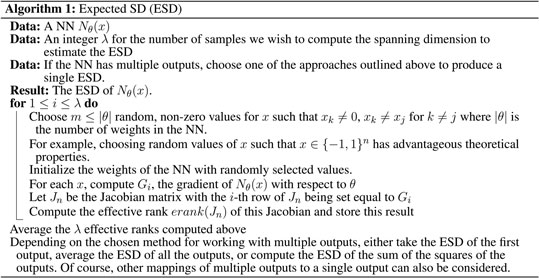
Figure 1 shows the SD distributions for an MLP with three hidden layers, one input and output, and 8, 8, and 10 nodes for the first, second, and third hidden layers, respectively. Figure 1A shows the SD distribution for this MLP with ReLU activation functions with an ESD of 2.81, and Figure 1B shows the SD for this MLP with sigmoid activation functions with an ESD of 1.07. We see that the SD of the MLP with ReLU activation functions, which are not smooth, varies much more than the MLP with sigmoid activation functions. Furthermore, even though both MLPs have the same number of trainable parameters, the MLP with sigmoid activation functions has a much lower ESD.

FIGURE 1

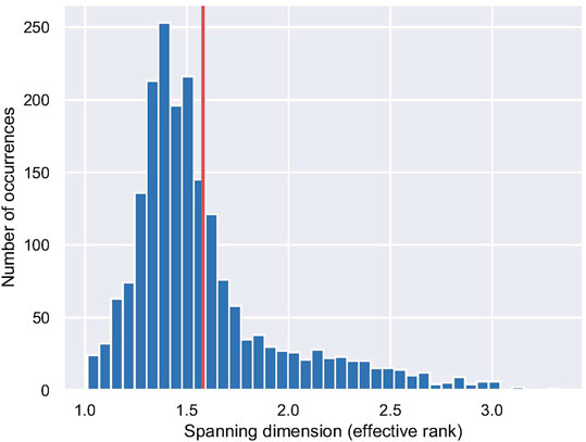
FIGURE 1. Estimated spanning distribution for an MLP with (A) ReLU activation functions, and (B) sigmoid activation functions.

Note, in the case of nonsmooth activation functions, the SD can change if the NN is evaluated at points that bracket a singularity in an activation function such as ReLU. However, as we show in Section 6, the ESD is quite stable even for real-world networks with nonsmooth activation functions.

3.2 Multiple Inputs and Outputs

Here, we address our third assumption above, that $N_{\theta }\left(x\right)$ has one input and one output. The method outlined in Section 3.1 naturally extends to NNs with more than one input. In this case, x is a vector instead of a scalar, and we still compute the gradient of this NN with respect to the weights of the NN. In our experimental results below, we use this approach to compute the SD of NNs with multiple inputs.

However, this approach does require that there is only one scalar output. To compute the ESD of an NN with multiple outputs, we recommend one of the following approaches.

(1) Compute the ESD of each output and then average the results. This is the most computationally expensive approach for larger networks.

(2) Compute the ESD of the first output. This approach is the least expensive computationally.

(3) Compute the ESD of the sum of squares of the outputs. This approach closely resembles the type of squared loss function used in regression problems.

In Section 6, we will provide numerical results on real-world networks that explore cases 2 and 3.

3.3 Singular Values and Connections to the Riesz Representation Theorem

Previously, when considering exact rank, we did not need to determine the actual magnitude of the singular values. However, when considering effective rank, these singular values are important.

Looking at 7 and Definition 1, some readers might be reminded of ideas such as the Riesz representation theorem [22]. In particular, as we pointed out earlier, when we define the PSD in Definition 1 in terms of the decomposition $N_{\theta }\left(x\right)=\text{Φ}{\left(x\right)}^{T}P\left(\theta \right)$, we are merely applying a finite dimensional version of the Riesz representation theorem [17]. The idea of the Riesz representation theorem is that such decompositions are actually quite general, and the Riesz representation theorem is an important part of the theory of infinite dimensional Hilbert spaces of functions [17].

Deriving such ideas in the Hilbert space setting would take us too far afield for the current context. However, there is one idea that is inspired by such considerations that we will leverage here. In particular, it is important to note that the expansion 2 is only one such possible expansion of the function $N_{\theta }\left(x\right)$. In 2, $N_p\left(x\right)$ was expanded in terms of the standard polynomial basis $1,x,x^2,\cdot$, but there are many other bases of the space of all polynomials, such as the Legendre basis and the Chebyshev basis [21].

The fact that there are many decompositions of $N_{\theta }\left(x\right)$ leads to many decompositions of $J_n$ into $V\left(x\right)J_c\left(\theta \right)$, where we have chosen our notation to emphasize the fact that $V\left(x\right)$ is purely a function of x, and represents some function basis of interest, and that $J_c\left(\theta \right)$ is purely a function of the parameters θ, and represents coefficients of the particular linear combination of the basis function that represents $N_{\theta }\left(x\right)$.

We are now interested in computing the eigenstructure of $J_c$ for determining the effective rank. However, as opposed to the simple example in $N_p\left(x\right)$, we will not necessarily have explicit access to a decomposition such as 7, but we will only be able to compute the gradient of an NN at particular values of x using backpropagation. In effect, we do not have direct access to the Jacobian whose eigenstructure we wish to compute, we instead can only access information about the Jacobian by computing dot products of the Jacobian with vectors x and then observing the result. Fortunately, as discussed in [25], the eigenstructure of a linear operator can indeed be estimated using such dot products. These methods are akin to many other matrix-free methods in linear algebra in which calculations can be preformed on a matrix which is not directly available, but only accessible through some function that can apply the unknown matrix to a vector [25]. However, our case is somewhat more complicated, since the eigenstructure of $J_c$ is masked by the eigenstructure of the polynomial basis matrix $V\left(x\right)$.

Fortunately, we have a trick that we can leverage. In the decomposition $J_n=V{J}_c$, we know that any sufficiently large full rank V will leave the rank of $J_n$ (which we can compute) and the rank of $J_c$(which we wish to know) the same. However, V can certainly cause the numerical values of the singular values of $J_n$ and $J_c$ to be different. The question then becomes how to reduce the impact of a choice of the polynomial basis V on the eigenstructure of $J_c$?

Since we do not have access to the decomposition $N_{\theta }\left(x\right)=\text{Φ}{\left(x\right)}^{T}P\left(\theta \right)$ for real-world NNs, and we have no a priori reason to prefer a particular basis, we are free to interpret the SD in terms of any convenient $\text{Φ}\left(x\right)$and to choose our samples x with advantageous properties. In particular, for many polynomials bases, such as the standard basis, each basis function evaluated at $x\in {\left\{-\mathrm{1,1}\right\}}^n$ (i.e., a vector x each of whose entries is $-1$ or 1) leads to a result which is also in $\left\{-\mathrm{1,1}\right\}$. For example, if we have a scalar $x\in \left\{-\mathrm{1,1}\right\}$ then for the standard basis we have that $x^0=1\in \left\{-\mathrm{1,1}\right\}$, $x^1\in \left\{-\mathrm{1,1}\right\}$, $x^2=1\in \left\{-\mathrm{1,1}\right\}$, $x^3\in \left\{-\mathrm{1,1}\right\}$, and so on. A similar construction holds for several other standard polynomial bases such as the Legendre basis and the Chebyshev basis of the first kind [21].

So, in our calculations, we are free to choose to interpret$N_{\theta }\left(x\right)=\text{Φ}{\left(x\right)}^{T}P\left(\theta \right)$ in terms of a $\text{Φ}\left(x\right)$ arising from either the standard, Legendre, or first-kind Chebyshev basis. In all these cases, for the choice of random$x\in {\left\{-\mathrm{1,1}\right\}}^n$, we know that every entry of our V will also be in$\left\{-\mathrm{1,1}\right\}$. While such a V in not guaranteed to be unitary, it is the case that interpreting $\text{Φ}\left(x\right)$ as one of the above bases and using $x\in {\left\{-\mathrm{1,1}\right\}}^n$ will lead to rows of $\text{Φ}\left(x\right)$ with constant norm. While not eliminating the impact of the choice of $\text{Φ}\left(x\right)$ on our Jacobian $J_n=\widehat{V}{J}_c$, we have found that this choice of $x\in {\left\{-\mathrm{1,1}\right\}}^n$ to reduces the noise in the numerical calculation of the SD of $J_n$.

3.4 Expected Spanning Dimension Algorithm

We are now ready to present the full algorithm for computing the ESD of $N_{\theta }\left(x\right)$. Algorithm 1 details the steps to compute ESD for an NN. This will be the key tool in our numerical studies in the rest of this article.

3.5 Comparing Effective Rank vs. Actual Rank

Figure 2 shows the estimated spanning dimension distribution for the simple NN from Eq. 1. We see that the ESD (1.59) is significantly smaller than the PSD (4.0). Effective rank does not just consider the number of nonzero singular values; it considers the relative magnitude of these singular values. This distribution of effective rank over the expected range of data inputs and weights provides a rich set of information for the given NN. Effective rank is always less than or equal to the actual rank and can be much smaller if many of the singular values are close to zero. Considering the singular value decomposition of the Jocobian, we can interpret the Jacobian as a rotation or reflection followed by a scaling followed by another rotation or reflection. The singular values represent the amount we move in each dimension during a backpropagation step. Whereas the actual rank considered only how many of these dimension we can move at all, effective rank considers how much we can move in each dimension.

FIGURE 2

FIGURE 2. Estimated spanning dimension distribution (effective rank) with 2,000 samples of a neural network with $f\left(z\right)=z^2$ activation functions, one node per hidden layer, one input, one output, and two hidden layers with expected spanning dimension 1.59.

4 Multilayer Perceptrons

In this section, we explore the relationship between ESD and learning capacity in terms of training error for multilayer perceptrons. ESD measures the expressiveness of an NN, its ability to fit input data points. An experimental framework was created to investigate this relationship.

For these experiments, a set of eight random input and output points were generated $x_1,x_2,\dots x_8$, $y_1,y_2,\dots y_8$, ensuring that $abs\left(x_i-x_j\right)>0.0001,i\ne j$. These points were used as training data. Two hundred randomly generated multilayer perceptrons were generated. These NNs were generated by first choosing a random number of hidden layers $l\in \left[\mathrm{1,6}\right]$, for each layer, choosing a random number of nodes $n_i\in \left[\mathrm{2,30}\right],i\in [1,l]$, and then choosing one of the following activation functions for each layer, tanh, ReLU, or sigmoid. For each of these MLPs, we computed the ESD and then used stochastic gradient descent to try and fit these eight random points. Our goal was to find the closest fit we could to the training data so we used stochastic gradient descent with 10 initial seeds and then chose the lowest training error of these 10 experiments.

Figures 3 and 4 show the results of these experiments. There is a very strong relationship between the training error and the ESD with a correlation of $-0.91$ and a p-value of $1.2\times {10}^{-70}$. In comparison, the relationship between training error and the number of trainable weights in the network is much weaker with a correlation of $-0.35$ and a p-value of $5.3\times {10}^{-7}$. Having more trainable parameters in no way guarantees that one will be able to fit the data more closely.

FIGURE 3

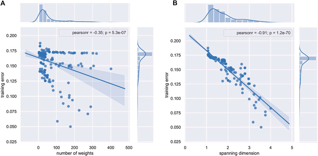
FIGURE 3. Training error vs. (A) number of trainable weights and (B) ESD for 200 randomly generated multilayer perceptrons.

FIGURE 4

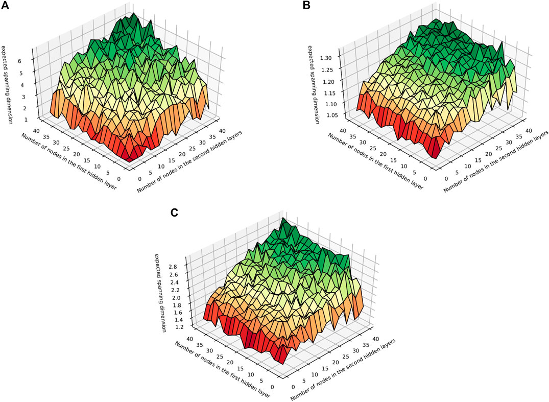
FIGURE 4. The ESD for all MLPs with two hidden layers and nodes per hidden layer less than or equal to 40 with activation function ReLU, sigmoid, or tanh.

4.1 Analyzing Multilayer Perceptrons With Two Hidden Layers

In this section, we describe the results of an exhaustive set of experiments that were run to investigate the ESD of 4800 multilayer perceptrons. For each activation function, sigmoid, ReLU, and tanh, we compute the ESD of all multilayer perceptron with two hidden layers where the first and second hidden layers have i and j nodes, respectively, with $i,j\in \left[\mathrm{1,40}\right]$.

These results show that in general ReLU has a much higher ESD than sigmoid and tanh, and may partly explain why ReLU tends to perform well in deep NNs. Sigmoid in contrast has a very low ESD and appears to plateau earlier. In particular, both sigmoid and tanh, unlike ReLU, do not appear to have a significantly higher ESD when the first hidden layer has more nodes. The number of nodes in the second hidden layer has a greater impact on ESD.

4.2 Increasing the Expected Spanning Dimension of Multilayer Perceptrons

Consider the simple multilayer perceptron in Figure 5A. This multilayer perceptron with three inputs, two hidden layers, one output, three nodes per hidden layer, and sigmoid activation function has 27 weights and an ESD of 2.76.

FIGURE 5

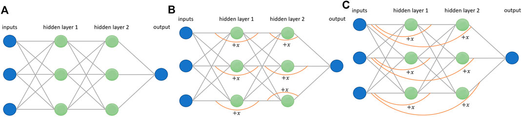
FIGURE 5. (A) A multilayer perceptron with ESD 2.76, (B) adding shortcut paths increases ESD to 4.28, and (C) adding inputs directly to the outputs of the hidden nodes increases ESD to 4.69.

Perhaps, we wish to have a more flexible NN that can represent a larger family of functions. Interestingly, the ESD can be increased without adding weights, merely by adding links similar to those found in ResNets [26]. The full justification of this idea is a subject of future work, but perhaps intuition can be gained by looking back at 2. One may observe that the coefficient in front of the high-order terms with respect to x are high-order polynomials with respect to the coefficients of the NN. It is our experience that such terms lead to low ESD. By adding additional links, additional low-order terms with respect to the higher powers of x are added, increasing the ESD.

Figure 5B shows a multilayer perceptron with shortcut pathways added that skip over the hidden neurons. The input of each hidden neuron is added directly to the output of that same neuron, skipping the multiplication of the weight, the bias term, and the activation function. Adding these extra pathways results in a significant increase of the ESD to 4.28. We call an NN with these extra pathways an add-shortcuts NN.

If adding these shortcuts increases the ESD considerably, a natural extension of this idea is to replace the smaller shortcuts with larger ones that skip over more of the hidden neurons. In fact, inspired by DenseNets [27], we create shortcuts that go directly from the inputs of the NN to the output of each hidden node, as shown in Figure 5C. The inputs of each row in the NN are added directly to the output of each node in the hidden layers. We call this an add-inputs NN. This results in a further increase of the ESD from 4.28 to 4.69.

It is interesting to note that, from the perspective of ESD, the modifications to standard NN architectures used by high-performance networks such as ResNets [26] and DenseNets [27] seem well justified, as opposed to more ad hoc arguments that are sometimes made with regard to these networks.

5 Results on Benchmark Datasets

In this section, we modify larger multilayer perceptrons by adding shortcuts as shown in Figure 5B. Then, we add inputs directly to the outputs of the hidden nodes as shown in Figure 5C. All experiments in this section were performed on an Alienware M15 laptop with an external Alienware amplifier with an NVIDIA GTX 2080 TI GPU.^a

5.1 Fitting Random Noise

To measure the fitting power of an NN, we test its ability to fit random noise given a certain number of inputs. One thousand images of size $28\times 28$ were generated with random noise and assigned to one of ten arbitrary classes. Three NNs were generated with three hidden layers and $28\times 28=784$ nodes per hidden layer. The first NN is a standard multilayer perceptron with sigmoid activation functions. The second NN adds shortcuts that skip over single hidden nodes to the first NN. We call this network an add-shortcuts network. The shortcuts that are added are similar to those found in ResNet (see [26]). The final NN, which we call the add-inputs network, adds shortcuts that go directly from the inputs to the outputs of the hidden nodes in the NN and, based upon our previous results, should have a larger ESD. This is similar to the procedure in Section 4.2, where the input in the same row of the NN is added to each hidden node in that same row as shown in Figure 5C.^b

Indeed, that is the case, and Figure 6 shows that only the add-inputs model is able to fit the noise with gradient descent, indicating that it has greater fitting power or variance than both the add-shortcuts model and the original multilayer perceptron.

FIGURE 6

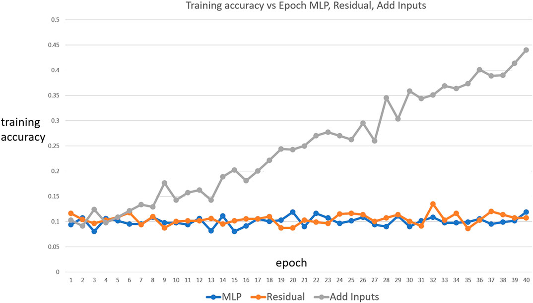
FIGURE 6. Fitting a multilayer perceptron, an add-shortcuts, and an add-inputs network to random noise images with ten arbitrary classes. The add-inputs model is able to fit the noise images while the other two models are not able to. Accordingly, this NN has more flexibility than the other networks, and can overfit.

FIGURE 7

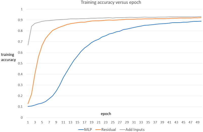
FIGURE 7. Fitting a multilayer perceptron, a residual network, and an add-inputs network to $\mathrm{10,000}$ MNIST images. With the additional training data using structured images the flexibility of the add-inputs network leads to better performance (see Table 1 for the testing accuracies).

5.2 Fashion MNIST

These three NN architectures were then trained on fashion MNIST images to determine the effect of increased ESD on performance in a practical setting [28]. Table 1 shows the training and testing accuracy of the multilayer perceptron, the add-inputs model, and the add-shortcuts model for various numbers of epochs. We observe that the testing accuracy is important for judging the performance of NNs, and we note that increasing ESD improves both the training and testing performance of the given NNs. This suggests that the original NN is actually, and perhaps surprisingly, under-fitting the data when only a small number of training epochs are used.

TABLE 1

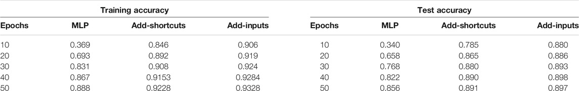
TABLE 1. Fashion MNIST training and test accuracy average of three runs comparing multilayer perceptron (MPL) to our proposed architectures.

The testing accuracy for these architectures is higher than both the multilayer perceptron and residual models in every test case. Each experiment was run 3 times, and the average training and test accuracies were computed.

5.3 Deep Residual Networks

Adding shortcuts that skip over individual nodes in a multilayer perceptron was inspired by deep residual networks [26]. As shown above, our findings indicate that replacing these shortcuts with larger shortcuts, which add the inputs directly to the outputs of the hidden neurons, increases ESD. Here, we investigated the effect of replacing some of these shortcuts in the ResNet architecture with these longer shortcuts. Our ResNet implementation is based upon that found in https://keras.io/examples/cifar10_resnet/. After each max pooling layer in the ResNet architecture, the size of the intermediate images decreases by a factor of 2. When this occurs, ResNet adds a subset of a previous layer by sampling every other pixel using a convolutional layer with kernel size 1 and stride 2. We replace these shortcuts with convolutional layers that sample the inputs directly with a stride of $2^n$, where n is the number of max pooling layers in between the input and the given hidden node. These two architectures have the same number of weights.

To see how well these NNs perform on a low number of training inputs, these two networks were trained on 3,000 images from the CIFAR-10 dataset for various numbers of epochs using stochastic gradient descent [29]. Figure 8 shows the training accuracy vs. number of epochs for the original ResNet architecture and the add-inputs model. Table 2 shows the final test accuracies for various experiments. For each experiment, the add-inputs model has a higher test accuracy than the original ResNet model. Again, we emphasize that increasing ESD again improves both the training and testing performance of the given NNs, and perhaps indicates that the original NN is also under-fitting the data in this case.

FIGURE 8

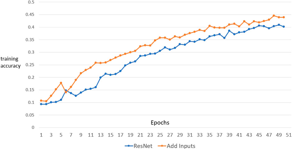
FIGURE 8. Fitting the original ResNet architecture and the add-inputs model to 3,000 images from the CIFAR-30 dataset. The add-inputs model learns faster and has a higher final test accuracy than the ResNet network.

TABLE 2

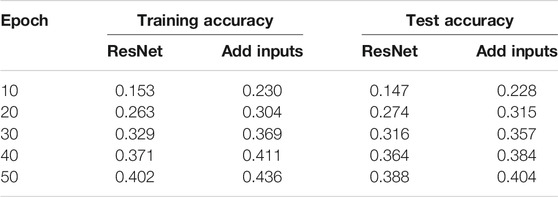
TABLE 2. CIFAR-10 training and test accuracy average of three runs.

6 The Expected Spanning Dimension of Real-World Neural Networks

In previous sections, we have demonstrated the ESD on NNs of our own construction and have focused largely on training error as a measure of the flexibility of an NN. However, these ideas can be applied to arbitrary NNs. In this section, we demonstrate the application of the ESD to eighteen NNs from the literature as implemented by the PyTorch NN library [22] in torchvision.models [30]. Our goal here is to look at the testing error of larger NNs widely used in practice. We might expect that if the ESD is too high, then over-fitting might occur and the testing error will increase. In this section, we show that over-fitting does not appear to be occurring with these real-world NNs. There are a significant number of variables and challenges when measuring the testing error of an NN including difficulty of training, limitations of the learning algorithm, structure and distribution of the input data, size of training data, and outliers in the training data. Despite all of this noise, we see a negative correlation between ESD and testing error. These experiments were conducted on a multi-node high-performance computing system with a variety of Intel-based processors and NVIDIA K20 GPUs.^c The network families we examine include

(1) VGG (versions 11, 13, and 19) [31],

(2) ResNet (versions 18, 34, 50, 101, and 152) [32],

(3) SqueezeNet (versions 1.0 and 1.1) [33],

(4) DenseNet (versions 121, 161, 169, 201) [27],

(5) ShuffleNet (version 2-1.0) [34],

(6) MobileNet (version 2) [35], and

(7)ResNext (versions 50 and 101) [36].

Each NN f that we consider has been implemented to ingest RGB images x of size $3\times 224\times 224$ from the ImageNet dataset and output a probability vector y of size 1,000, with each entry being the probability of 1,000 possible image classifications. We have for each NN a function of the following form, $f:{\mathrm{ℝ}}^{3\text{*}224\text{*}224}\to {\mathrm{ℝ}}^{1000}$.

To demonstrate the effectiveness of our methodology, we choose NNs with a number of parameters that range over several orders of magnitude. We choose networks that range in size from just over one one million parameters to networks with over 100 million parameters. We will denote by θ the set of all parameters of the network, so each network can be written as $f_{\theta }\left(x\right)=y$.

To handle the multiple outputs of each NN, we compute the ESD using two of the approaches outlined in Section 3.1. In these calculations, we wish to compute a single Jacobian for each NN, and so we turn each NN into a function g with a scalar output by setting.

(1) $g_{\theta }\left(x\right)=f_{\theta }{\left(x\right)}_1$ (what we will later call pick_1st), or

(2) $g_{\theta }\left(x\right)={{{\displaystyle \sum }}^{\text{}}}_{i=1}^{1000}{f}_{\theta }{\left(x\right)}_i^2$ (what we will later call sum_squares).

With the above notation in mind, our experiments proceed as follows.

We choose, at random, a set of $\mathrm{1,000,000}$ entries of the gradient of $g_{\theta }$.

We generate these $\mathrm{1,000,000}$ entries of the gradient for 500 different random choices of x and call this $500\times \mathrm{1,000,000}$ matrix J. For each row of J we choose $x\in {\left\{-\mathrm{1,1}\right\}}^{3\times 224\times 224}$ as suggested in Section 3.3 (shown in Figures 9 and 10) or x as an image from the ImageNet dataset (shown in Figures 11 and 12).

In an optimization of Algorithm 1 to save memory for large NNs, we compute the singular values of $J_n$ by first computing the Gram matrix $J_n{J}_n^T$, computing the singular values of $J_n{J}_n^T$, and taking their square roots.

FIGURE 9

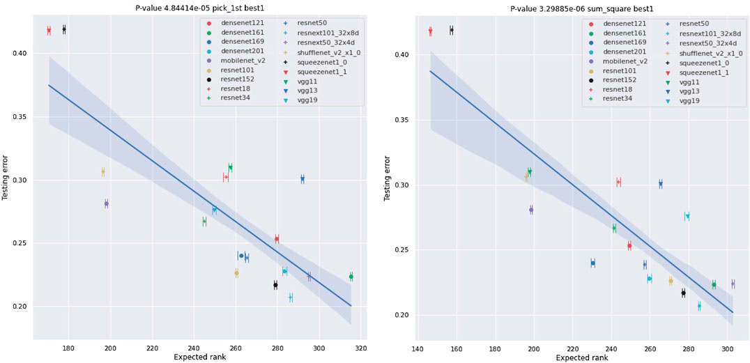
FIGURE 9. Plots of the best-1 testing error of NNs against their ESD. The testing errors are as provided by [30] and are error rates for testing on ImageNet crop images. We also provide the range of the ESD over 10 different experiments using synthetic data of the form $x\in {\left\{-\mathrm{1,1}\right\}}^{3\times 224\times 224}$, and, as can be observed, the ranges are quite small relative to the differences between the various networks. In addition, the ESD shows a strong negative correlation with the best-1 error. The confidence bounds on the linear fit are one-σ bounds based on 1,000 bootstrap samples.

FIGURE 10

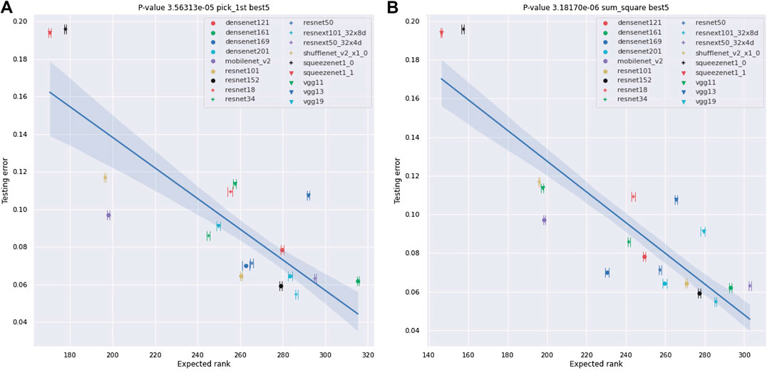
FIGURE 10. Plots of the best-5 testing error of NNs against their ESD. As in Figure 9, the testing errors are as provided by [30] and are error rates for testing on ImageNet crop images. We also provide the range of the ESD over 10 different experiments using synthetic data of the form $x\in {\left\{-\mathrm{1,1}\right\}}^{3\times 224\times 224}$, and, again, the ranges are quite small relative to the differences between the various networks. Also in this case, the ESD shows a strong negative correlation with the best-5 error. The confidence bounds on the linear fit are one-σ bounds based on 1,000 bootstrap samples.

FIGURE 11

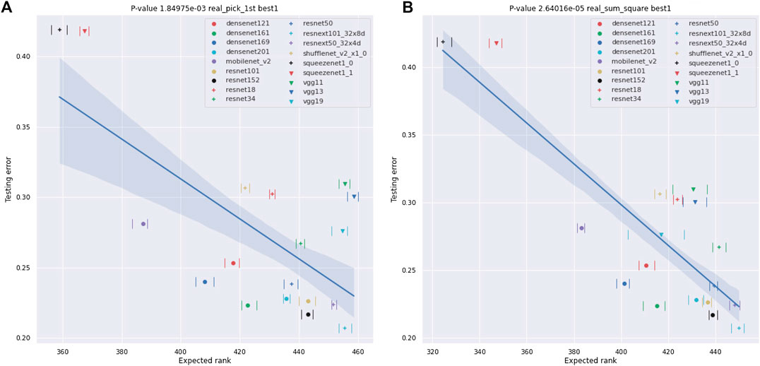
FIGURE 11. Plots of the best-1 testing error of NNs against their ESD. As in Figure 9, the testing errors are as provided by [30] and are error rates for testing on ImageNet crop images. We also provide the range of the ESD over 10 different experiments using an image from the ImageNet dataset for each x, and, again, the ranges are small relative to the differences between the various networks, though somewhat larger than in the $x\in {\left\{-\mathrm{1,1}\right\}}^{3\times 224\times 224}$. Also in this case, the ESD shows a strong negative correlation with the best-1 error. It is interesting to note that the ranges of the ESD for each NN are larger in this case than in 9 and 10. We conjecture that this is because of the larger diversity of the ImageNet dataset. However, the p-values are still quite small, even in this case. The confidence bounds on the linear fit are one-σ bounds based on 1,000 bootstrap samples.

FIGURE 12

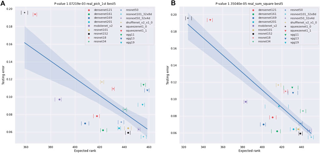
FIGURE 12. Plots of the best-5 testing error of NNs against their ESD. As in Figure 9, the testing errors are as provided by [30] and are error rates for testing on ImageNet crop images. We also provide the range of the ESD over 10 different experiments using an image from the ImageNet dataset for each x, and, again, the ranges are quite small relative to the differences between the various networks, though somewhat larger than in the $x\in {\left\{-\mathrm{1,1}\right\}}^{3\times 224\times 224}$. Also in this case, the ESD shows a strong negative correlation with the best-5 error. It is again interesting to note that the ranges of the ESD for each NN are larger in this case then in 9 and 10. We conjecture that this is because of the larger diversity of the ImageNet dataset. However, the p-values are still quite small, even in this case. The confidence bounds on the linear fit are one-σ bounds based on 1,000 bootstrap samples.

This provides one set of singular values. We then iterate this procedure 10 times to get 10 sets of 500 singular values for each NN. Note, the choice of 500 in the above algorithm is not essential to the performance of the algorithm, and many different choices were tried as part of our experiments. 500 was chosen in this case as all singular values for all networks past this point are small.

Fortunately, PyTorch makes the computation of $J_n$ from a particular NN simple by way of their torch.autograd.grad function. This function exposes an API for computing arbitrary derivatives of NNs with respect to both x and θ analytically using the chain rule. Finally, as opposed to the simple examples in “A Simple Example to Inspire the Approach” section, the numerically computed Jacobians are of higher rank.

Our results for real-world NNs can be found in Figures 9-13 and Tables 3 and 4. In these figures, we plot the ESDs of the 18 NNs we examine against their testing error, as provided by the PyTorch torchvision library [30], along with their least-squares fitting line. The ESDs are quite predictive of the NNs best-1 and best-5 errors, with p-values’ orders of magnitude lower than the classic statistical significance limit of 0.05. The sum_squares method provides a stronger relationship between ESD and testing error vs. the pick_first method. The correlation between the testing error and the number of parameters in the NN is much weaker, with p-values of only 0.553 for the best-1 error and 0.478 for the best-1 error.

FIGURE 13

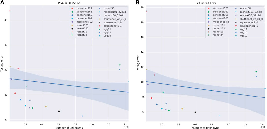
FIGURE 13. Plots of the best-1 and best-5 testing errors of NNs against the number of parameters. Again, the testing errors are as provided by [30] and are error rates for testing on ImageNet crop images. The number of parameters in the network is not a statistically significant predictor of their performance. The confidence bounds on the linear fit are one-σ bounds based on 1,000 bootstrap samples.

TABLE 3

TABLE 3. p-Values for the linear relationship between ESD and accuracy over several different scenarios including examples using both synthetic data and real ImageNet data.

TABLE 4

TABLE 4. Comparison between the p-values for the number of parameters and ESD for predicting testing accuracy.

A concise summary of the results for analyzing NNs with ESDs can be found in Tables 3 and 4. In particular, we show results for all possible combinations of best-1 vs best-5 accuracies, our two vector to scalar mappings, pick_first and sum_squares, and real and synthetic data. Our results show high correlations in all of these cases between our ESD-based measures and the accuracies of the 18 NNs, with the lowest p-values for all “sum-squares” examples being less than 5.0e−5, which is 3-orders of magnitude smaller than the classic limit of 5.0e−2. We also show, in Table 4, that ESD results are robust to selecting different subsets of the NNs we analyze.

7 Conclusions

In this article, we have defined the idea of an ESD for NNs and have demonstrated how maximizing this ESD improves the performance of real-world NNs. In many ways, a small ESD can be thought of as a regularization of the NN, and increasing the ESD is an example of the bias–variance trade-off in machine learning. ESD can be controlled by judiciously including additional links in the NN and does not require changing the number of parameters in the NN. Perhaps, most importantly, an ESD analysis provides a mathematical foundation for the superior performance of ResNet type NNs. There are many possible directions for augmenting the results described here. For example, Theorem 2.1 only scratches the surface of the theoretical progress that can be made using ESD-type ideas for the understanding of NNs, and the bounding of the ESD is certainly a worthwhile direction for future work. However, such results appear to be nontrivial, except in the smallest of cases. In particular, the example can be analyzed in terms of algebraic geometry using Gröbner bases [37] and similar ideas. However, generating such results for activation functions with infinite Taylor series has so far proved nontrivial. We expect that such analysis can lead to superior NN architectures in many problem domains.

As a final point, the interpretation of the ESD in context of the recent work in “double descent” is a delicate and quite interesting direction for future work. In particular, several of our results demonstrate that the testing accuracy of NNs improves as the ESD increases. There are two explanations that present themselves. First, large-scale NNs are actually somewhat under-parameterized or, more precisely, have access to far fewer degrees of freedom than their number of unknowns would indicate. Their performance is therefore improved by the additional flexibility that a larger ESD provides. Second, large-scale NNs are already in the “double descent” range and increasing ESD is taking advantage of this fact. Resolving this question would likely take a delicate computational study involving the development of a technique for slowly increasing the ESD in a large-scale NN.

Data Availability Statement

Publicly available datasets were analyzed in this study. These data can be found here: http://www.pymvpa.org/datadb/mnist.html, https://www.cs.toronto.edu/∼kriz/cifar.html, https://pytorch.org/docs/stable/torchvision/index.html.

Author Contributions

The core of writing of this article was performed by DB and RP. The numerical results included in the article were generated by DB and RP, with additional numerical results that inspired some of the approaches presented in the article being generated by LG. The key ideas in the article were generated through discussions between DB and RP, and RP and LG.

Conflict of Interest

The authors declare that the research was conducted in the absence of any commercial or financial relationships that could be construed as a potential conflict of interest.

Acknowledgments

This research was performed using computational resources supported by the Academic and Research Computing group at Worcester Polytechnic Institute. The authors would also like to acknowledge the Academic and Research Computing group at Worcester Polytechnic Institute for providing consulting support that contributed to the results reported within this article.

Footnotes

^aAll codes for experiments are available upon request.

^bIn the notation of [26], add-shortcuts would be F(x) + x and add-inputs would be F(x) + x₀ where x₀ is the input layer.

References

1. Canziani, A, Paszke, A, and Culurciello, E. An analysis of deep neural network models for practical applications. CoRR (2016). abs/1605, 07678.

Google Scholar

2. Schelkes, L. Evaluation of neural networks for image recognition applications: designing a 0-1 MILP model of a CNN to create adversarials. CoRR (2018). abs/1809, 00216.

Google Scholar

3. Sard, A. The measure of the critical values of differentiable maps. Bull Am Math Soc (1942). 48(12), 883–891. doi:10.1090/s0002-9904-1942-07811-6

CrossRef Full Text | Google Scholar

4. Ouarti, N, and Carmona, D. Out of the black box: properties of deep neural networks and their applications. CoRR (2018). abs/1808, 04433

Google Scholar

5. Neal, B, Mittal, S, Baratin, A, Tantia, V, Scicluna, M, Lacoste-Julien, S, et al. ,. A modern take on the bias-variance tradeoff in neural networks. CoRR (2018). abs/1810, 08591.

Google Scholar

6. Zhang, C, Bengio, S, Hardt, M, Recht, B, and Vinyals, O. “Understanding deep learning requires rethinking generalization,” in 5th International conference on learning representations, ICLR, Toulon, France, April 24–26, 2017, (2017).

Google Scholar

7. Mei, S, and Montanari, A. The generalization error of random features regression: Precise asymptotics and double descent curve. (2019). arXiv preprint arXiv:1908.05355.

Google Scholar

8. Belkin, M, Hsu, D, Ma, S, and Mandal, S. Reconciling modern machine learning and the bias-variance trade-off. (2018). arXiv preprint arXiv:1812.11118.

Google Scholar

9. Belkin, M, Hsu, D, and Xu, J. Two models of double descent for weak features. (2019). arXiv preprint arXiv:1903.07571.

Google Scholar

10. Thomas, V, Pedregosa, F, van Merriënboer, B, Mangazol, P.-A, Bengio, Y, and Roux, NL. Information matrices and generalization. (2019). arXiv preprint arXiv:1906.07774.

Google Scholar

11. Neyshabur, B, Bhojanapalli, S, McAllester, D, and Srebro, N. “Exploring generalization in deep learning,” in Advances in neural information processing systems, pp. 5947–5956 (2017).

Google Scholar

12. Wojtowytsch, S, et al. . Kolmogorov width decay and poor approximators in machine learning: shallow neural networks, random feature models and neural tangent kernels. (2020). arXiv preprint arXiv:2005.10807.

Google Scholar

13. Guss, WH, and Salakhutdinov, R. On characterizing the capacity of neural networks using algebraic topology. (2018). arXiv preprint arXiv:1802.04443.

Google Scholar

14. Hochreiter, S., and Schmidhuber, J. Flat minima. Neural Comput (1997). 9(1), 1–42. doi:10.1162/neco.1997.9.1.1

CrossRef Full Text | Google Scholar

15. Novak, R, Bahri, Y, Abolafia, DA, Pennington, J, and Sohl-Dickstein, J. Sensitivity and generalization in neural networks: an empirical study. (2018). arXiv preprint arXiv:1802.08760.

Google Scholar

16. Khan, A, Sohail, A, Zahoora, U, and Qureshi, AS. A survey of the recent architectures of deep convolutional neural networks. Artif Intell Rev (2020). 17, 1–62.

Google Scholar

17. Halmos, PR. Measure theory, Vol. 18. New York, NY:Springer (2013).

Google Scholar

18. Saxe, AM, McClelland, JL, and Ganguli, S. Exact solutions to the nonlinear dynamics of learning in deep linear neural networks. (2013). arXiv preprint arXiv:1312.6120.

Google Scholar

19. Meurer, A, Smith, CP, Paprocki, G, Čertík, O, Kirpichev, SB, Rocklin, M, et al. . Sympy: symbolic computing in python. PeerJ Comput Sci (2017). 3, e103.

Google Scholar

20. Nair, V, and Hinton, GE. “Rectified linear units improve restricted Boltzmann machines,” in Proceedings of the 27th international conference on machine learning (ICML-10), pp. 807–14 (2010).

Google Scholar

21. Stoer, J, and Bulirsch, R. Introduction to numerical analysis, Vol. 12. Berlin: Springer Science & Business Media (2013).

Google Scholar

22. Paszke, A, Gross, S, Chintala, S, Chanan, G, Yang, E, DeVito, Z, et al. . Automatic differentiation in pytorch (2017).

Google Scholar

23. Glorot, X, Bordes, A, and Bengio, Y. “Deep sparse rectifier neural networks,” in Proceedings of the fourteenth international conference on artificial intelligence and statistics, pp. 315–323 (2011).

Google Scholar

24. Roy, O, and Vetterli, M. “The effective rank: a measure of effective dimensionality,” in 2007 15th European signal processing conference, New York, NY: IEEE, pp. 606–610 (2007).

Google Scholar

25. Halko, N, Martinsson, N. G, and Tropp, J. A. Finding structure with randomness: probabilistic algorithms for constructing approximate matrix decompositions. SIAM Rev. (2011). 53(2), 217–288. doi:10.1137/090771806

CrossRef Full Text | Google Scholar

26. He, K, Zhang, X, Ren, S, and Sun, J. Deep residual learning for image recognition. CoRR (2015). abs/1512 03385.

Google Scholar

27. Huang, G, Liu, Z, Van Der Maaten, L, and Weinberger, KQ. “Densely connected convolutional networks,” in Proceedings of the IEEE conference on computer vision and pattern recognition, pp. 4700–4708 (2017).

Google Scholar

28.Lecun. The mnist dataset of handwritten digits (images)—pymvpa 2.6.5.dev1 documentation (1999). Available at: http://www.pymvpa.org/datadb/mnist.html. (Accessed April 22 2019).

Google Scholar

29.Cifar-10 and cifar-100 datasets. Cifar-10 and cifar-100 datasets (2019). Available at: https://www.cs.toronto.edu/∼kriz/cifar.html. (Accessed April 22, 2019).

Google Scholar

30. Marcel, S., and Rodriguez, Y. “Torchvision the machine-vision package of torch,” in Proceedings of the 18th ACM international conference on Multimedia, ACM (2011). pp. 1485–1488.

Google Scholar

31. Simonyan, K., and Zisserman, A. Very deep convolutional networks for large-scale image recognition. (2014). arXiv preprint arXiv:1409.1556.

Google Scholar

32. He, K, Zhang, X, Ren, S, and Sun, J. “Deep residual learning for image recognition,” inProceedings of the IEEE conference on computer vision and pattern recognition, pp. 770–778 (2016).

Google Scholar

33. Iandola, FN, Han, S, Moskewicz, MW, Ashraf, K, Dally, WJ, and Keutzer, K. Squeezenet: Alexnet-level accuracy with 50x fewer parameters and¡ 0.5 mb model size. (2016). arXiv preprint arXiv:1602.07360.

Google Scholar

34. Ma, N, Zhang, X, Zheng, H.-T, and Sun, J.“Shufflenet v2: practical guidelines for efficient cnn architecture design,” in Proceedings of the European Conference on computer vision (ECCV), pp. 116–131 (2018).

Google Scholar

35. Sandler, M, Howard, A, Zhu, M, Zhmoginov, A, and Chen, L.-C. “Mobilenetv2: Inverted residuals and linear bottlenecks,” inProceedings of the IEEE Conference on computer Vision and pattern recognition, pp. 4510–4520 (2016).

Google Scholar

36. Xie, S, Girshick, R, Dollár, P, Tu, Z, and He, K. “Aggregated residual transformations for deep neural networks” in Proceedings of the IEEE conference on computer vision and pattern recognition, pp. 1492–500 (2017).

Google Scholar

37. Adams, WW, Adams, WH, Loustaunau, P, and Adams, WW. An introduction to Grobner bases. No. 3. Providence, RI: American Mathematical Society (1994).

Google Scholar