 Weizhi Zhu
 Yifei Huang
 Yuan Yao
- Department of Mathematics, The Hong Kong University of Science and Technology, Hong Kong, China
Margin enlargement of training data has been an important strategy for perceptrons in machine learning for the purpose of boosting the confidence of training toward a good generalization ability. Yet Breiman (1999) shows a dilemma: a uniform improvement on margin distribution does not necessarily reduce generalization errors. In this paper, we revisit Breiman's dilemma in deep neural networks with recently proposed spectrally normalized margins from a novel perspective based on phase transitions of normalized margin distributions in training dynamics. Normalized margin distribution of a classifier of the data can be divided into two parts: low/small margins such as some negative margins for misclassified samples vs. high/large margins for high confident correctly classified samples, which often behave differently during the training process. Low margins for training and test datasets are often effectively reduced in training, along with reductions of training and test errors, whereas high margins may exhibit different dynamics, reflecting the trade-off between the expressive power of models and the complexity of data. When data complexity is comparable to the model expressiveness, high margin distributions for both training and test data undergo similar decrease-increase phase transitions during training. In such cases, one can predict the trend of generalization or test error through margin-based generalization bounds with restricted Rademacher complexities, shown in two ways in this paper with early stopping time exploiting such phase transitions. On the other hand, over-expressive models may have both low and high training margins undergoing uniform improvements with a distinct phase transition in test margin dynamics. This reconfirms the Breiman's dilemma associated with over-parameterized neural networks where margins fail to predict overfitting. Experiments are conducted with some basic convolutional networks, AlexNet, VGG-16, and ResNet-18, on several datasets, including Cifar10/100 and mini-ImageNet.
1. Introduction
Margin, as a measurement of the robustness that allows some perturbations on classifiers without changing decisions on training data, has a long history in characterizing the performance of classification algorithms in machine learning. As early as [1], it played a central role in the proof on finite-stopping or convergence of perceptron algorithm when training data is separable. Equipped with the convex optimization technique, a plethora of large margin classifiers were triggered by support vector machines [2, 3]. For neural networks, Bartlett [4, 5] showed that the generalization error can be bounded by a margin-sensitive fat-shattering dimension, which is in turn bounded by the ℓ1-norm of weights, shedding light on the possible good generalization ability of over-parameterized networks with small weights despite the large VC dimensionality. The same idea was later applied to AdaBoost, an iterative algorithm to combine an ensemble of classifiers proposed by [6], often exhibiting a phenomenon of resistance to overfitting that, during the training process, the generalization error does not increase even when the training error drops to zero. In pursuit of deciphering such resistance to the overfitting phenomenon, Schapire et al. [7] proposed an explanation that the training process keeps on improving a notion of classification margins in boosting among later improvements [8] and works on establishing consistency of boosting via early stopping regularization [9–11]. Lately, such a resistance to overfitting was again observed in deep neural networks with over-parameterized models [12]. A renaissance of margin theory was brought by [13] with a normalization of networks using Lipschitz constants bounded by products of operator spectral norms. It has inspired many further investigations in various settings [14–16].
However, margin theory has a limitation that the improvement of margin distribution does not necessarily guarantee a better generalization performance, which is at least traced back to [17] in his effort to understand AdaBoost. In this work, Breiman designed an algorithm arc-gv such that the margin can be maximized via a prediction game. He then demonstrated an example that one can achieve uniformly larger margin distributions on training data than AdaBoost but suffer a higher generalization error. At the end of this paper, Breiman made the following comments with a dilemma:
“The results above leave us in a quandary. The laboratory results for various arcing algorithms are excellent, but the theory is in disarray. The evidence is that if we try too hard to make the margins larger, then overfitting sets in. ⋯ My sense of it is that we just do not understand enough about what is going on.”
In this paper, we are going to revisit Breiman's dilemma in the context of deep neural networks. We shall see margin distributions on training and test data may behave differently on the low and high parts during training processes. First of all, let us look at the following illustration example.
Example 1.1 (Breiman's Dilemma with a CNN). A basic five-layer convolutional neural network of c channels (see section 3 for details) is trained with the CIFAR-10 dataset whose 10% labels are randomly permuted as injected noises. When c = 50 with 92, 610 parameters, Figure 1A shows the training error and generalization (test) error in solid curves. From the generalization error in Figure 1A, one can see that overfitting indeed happens after about 10 epochs despite the training error continuously dropping to zero. One can successfully predict such an overfitting phenomenon from Figure 1B, which shows the evolution of normalized training margin distribution defined later in this paper. In Figure 1B, while low or small margins are monotonically improved during training, high or large margins undergo a phase transition from increase to decrease around 10 epochs such that one can predict the tendency of generalization error in Figure 1A using high margin dynamics. Two particular sections of high margin dynamics are highlighted in Figure 1B, one at 9.8 on x-axis, which measures the percentage of normalized training margins no more than 9.8 (training margin error), and the other at 0.8 on the y-axis, which measures the normalized margins at quantile q = 0.8 (i.e., defined later). Both of them meet the tendency of generalization error in Figure 1A and find a good early stopping time to avoid overfitting. However, as we increase the channel number to c = 400 by about 5.8M parameters and retrain the model, Figure 1C shows a similar overfitting phenomenon in terms of the generalization error; on the other hand, Figure 1D exhibits a uniform improvement of both low and high normalized margins without a phase transition during the training and thus fails to capture the overfitting. This demonstrates the Breiman's dilemma in wide CNN.
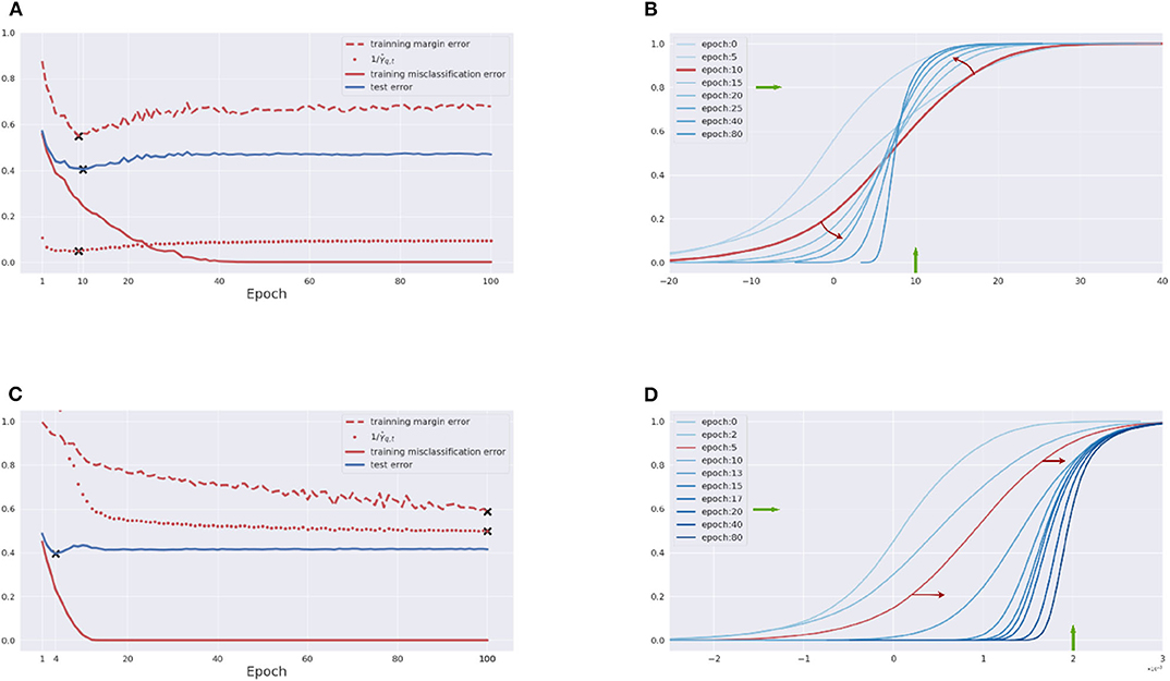
Figure 1. Demonstration of Breiman's dilemma in convolutional neural networks. CNN of 50 channels: (A) training and test error, training margin error, and inverse margins; (B) dynamics of training margin distributions. CNN of 400 channels: (C) training and test error, training margin error and inverse margins; (D) dynamics of training margin distributions. Details are shown in Example 1.1.
A key insight into this dilemma is that one needs a trade-off between the expressive power of models and the complexity of the dataset to endorse training margins as a prediction power. On one hand, when a model has a limited expressive power relative to the training dataset, in the sense that the low and high training margins cannot be uniformly improved during training, low margins can be effectively enlarged during training by reducing the training loss, though at the cost of sacrificing high margins, which does not affect the training loss as much as low margins, indicating misclassified samples. In this case, the generalization or test error may be predicted from dynamics of normalized training margin distributions by the increase-decrease phase transition that high margins experience. On the other hand, if we push too hard to improve margins by giving models too much degree of freedom such that the training margins are uniformly improved during training process, the predictability may be lost and overfitting set in. A trade-off is thus necessary to balance the complexity of model and dataset, otherwise one is doomed to meet Breiman's dilemma when the models arbitrarily increase the expressive power.
The example above shows that the expressive power of the models relative to the complexity of the dataset can be observed from the dynamics of normalized margins in training instead of counting the number of parameters in neural networks. In the sequel, our main contributions are to make these precise by revisiting the Rademacher complexity bounds on network generalization error.
• With the Lipschitz-normalized margins, a linear inequality is established between training margin and test margin in Theorem 1. When both training and test normalized margin distributions undergo similar phase transitions on increase-decrease during the training process, one may predict the generalization error based on the training margins, as illustrated in Figure 1.
• In a dual direction, one can define a quantile margin via the inverse of margin distribution functions to establish another linear inequality between the inverse quantile margins and the test margins, as shown in Theorem 2. Quantile margin is far easier to tune in practice and enjoys a stronger prediction power exploiting an adaptive selection of margins along model training.
• In all cases, Breiman's dilemma may fail both of the methods above when dynamics of normalized training margins undergo different phase transitions to that of test margins during training where a uniform improvement of training margins results in overfitting.
Section 2 describes our method to derive the two linear inequalities of generalization bounds above. Extensive experimental results are shown in section 3 with basic CNNs, AlexNet, VGG, ResNet, and various datasets, including CIFAR10, CIFAR100, and mini-Imagenet. Conclusions and future directions are discussed in section 4. More experimental figures and proofs are collected in Appendices.
2. Methodology
2.1. Definitions and Notation
Let be the input space [e.g., in image classification of size #(channel)-by-#(width)-by-#(height)] and be the space of K classes. Consider a sample set of n observations that are drawn i.i.d. from PX, Y. For any function , let be the population expectation and be the sample average.
Define to be the space of functions represented by neural networks:
where l is the depth of the network, Wi is the weight matrix corresponding to a linear operator on xi, and σi stands for either the element-wise activation function (e.g., ReLU) or pooling operator, which are assumed to be Lipschitz bounded with constant Lσi. An example would be the convolutional network Wixi + bi = wi * xi + bi where * stands for the convolution between the input tensor xl and kernel tensor wl. We equip with the Lipschitz semi-norm, that is, for each f,
where ||·||σ is the spectral norm and . Without loss of generality, we assume Lσ = 1 for simplicity. Moreover, we consider the following family of hypothesis functions as network mapping evaluated at (x, y),
where [·]j denotes the jth coordinate, and we further define the following class induced by Lipschitz semi-norm bound on ,
Now, rather than merely looking at whether prediction f(x) on y is correct or not, we further consider the prediction margin, which is defined as . With that, we can define the ramp loss and margin error depending on the confidence of predictions. Given two thresholds γ2 > γ1 ≥ 0, we define the ramp loss to be
where Δ: = γ2 − γ1. In particular γ1 = 0 and γ2 = γ, we also write ℓγ = ℓ(0, γ) for simplicity. Define the margin error to measure if f has margin no more than a threshold γ,
In particular, e0(f(x), y) is the common mis-classification error and 𝔼[e0(f(x), y)] = ℙ[ζ(f(x), y) < 0]. Note that e0 ≤ ℓγ ≤ eγ, and ℓγ is the Lipschitz bounded by 1/γ.
2.2. Rademacher Complexity and the Scaling Issue
The central question we try to answer is, can we find a proper upper bound to predict the tendency of the generalization error during training such that can stop the training early, near the epoch, so that ℙ[ζ(ft(x), y) < 0] is minimized?
We begin with the following lemma, as a margin-based generalization bound with network Rademacher complexity for multi-label classifications, using the uniform law of large numbers [8, 13, 18, 19].
Lemma 2.1. (Rademacher Complexity based Generalization Bound). Given a γ0 > 0, then, for any δ ∈ (0, 1) with probability at least 1−δ, the following holds for any with :
where
is the Rademacher complexity of function class with respect to n samples, and the expectation is taken over xi, εi, i = 1, ..., n.
Unfortunately, direct application of such a bound in neural networks with a constant γ0 will suffer from the so-called scaling issue. To see this issue, let us look at the following proposition as a lower bound of Rademacher complexity term.
Proposition 1. (Lower Bound of the Rademacher Complexity). Consider the networks with activation functions σ, where we assume σ is Lipschitz continuous and there exists x0 such that and exists. For any L > 0, then, it holds that
where C > 0 is a constant that does not depend on S.
This proposition extends Theorem 3.4 in [13] to general activation functions and a multi-class scenario, and the proof is presented in the Appendix.
The scaling issue refers to the fact that, if the network Lipschitz L → ∞, by this Lemma the upper bound (6) becomes trivial since . On the other hand, the gradient descent method with logistic regression (cross-entropy) loss [20] and exponential loss (boosting) [21] will drive weight estimates to approach infinity for max-margin classifiers when the data is linearly separable. In particular, the latter work shows the growth rate of weight estimates is log(t). As for the deep neural network with cross-entropy loss, the input of the last layer is usually viewed as several features extracted from the original input. Training the last layer with other layers being fixed is a logistic regression, and the feature is linearly separable as long as the training error achieves zero. Therefore, without any normalization, the hypothesis space during training has no upper bound on L, and the upper bound (6) is thus useless.
To solve the scaling issue, in the following we are going to present normalization of margins and restricted Rademacher complexity within a unit Lipschitz ball. We are going to see when such bounds are tight enough to predict generalization errors based on training data.
2.3. Generalization Bounds by Normalized Margins and Restricted Rademacher Complexity
The first remedy is to restrict our attention on by normalizing f with its Lipschitz semi-norm or some tight upper bound estimates. Note that a normalized network has the same mis-classification error as f for all C > 0. For the choice of C, it is difficult in practice to directly compute the Lipschitz semi-norm of a network; instead, some approximate estimates on the upper bound Lf in (2) are available as discussed in section 2.4.
In the sequel, let be the normalized network and be the corresponding normalized hypothesis function from (3). A simple idea is to regard as a constant when the model complexity is not over-expressive against data; one can then predict the tendency of generalization error via training the margin error of the normalized network, which avoids the scaling issue and the exact computation of Rademacher complexity. In the following we present two bounds, with one on normalized margin error bound as the direct application of Lemma 0.0.1 and the other on quantile margin error bound as the inverse of the former that turns out to be more effective in applications.
2.3.1. Normalized Margin Error Bound
The following theorem states that the probability of normalized test margins rather than γ1 is controlled by the percentage of normalized training margins less than γ2 > γ1 up to a constant if the Rademacher complexity of unit ball is not large.
Theorem 1. Given γ1 and γ2 such that γ2 > γ1 ≥ 0 and Δ: = γ2 − γ1 ≥ 0, for any δ > 0 with probability of at least 1−δ along the training epoch t = 1, …, T, the following holds for each ft:
where .
Remark 1. When we take γ1 = 0 and γ2 = γ > 0, the bound above becomes
Remark 2. Recently, Liao et al. [16] investigated for normalized networks the strong linear relationship between cross-entropy training loss and test loss when the training epochs are large enough. However, the bound here is applied to the whole training process for all epoch t, which enables us to find the early stopping time t* by looking at change points of in the dynamics of high training margin distributions that will be discussed below.
Theorem 1 says that one can bound the normalized test margin distribution by the normalized training margin distribution . In particular, one hopes to predict the trend of generalization (test) error by choosing γ1 = 0 and a proper γ> such that the high training margin errors enjoy a high correlation with a test error of up to a monotone transformation. The following facts make it possible to achieve this.
• First, we do not expect the bound; for example (10), is tight for every choice of γ > 0. Instead, we hope there exists some γ such that the training margin error almost changes monotonically with generalization error. This indeed happens when the model complexity is not too much where one cannot uniformly enlarge the high training margins. For example, Figure 5 below shows the existence of such γ when models are not too big by exhibiting rank correlations between training the margin error at various γ and the test error for a CNN trained on CIFAR10 dataset. Moreover, Figure 4 below shows that the training margin error at such a good γ successfully recovers the tendency of generalization error.
• Second, the normalizing factor is not necessarily an upper bound of Lipschitz semi-norm. The key point is to prevent the complexity term of the normalized network going to infinity. Since for any constant c > 0, normalization by works in practice where the constant could be absorbed to γ, we could ignore the Lipschitz constant introduced by general activation functions in the hidden layers.
However, such a strategy may fail. As shown by Example 1.1 using Figure 1 above, once the training margin distribution is uniformly improved, the dynamic of training margin error fails to capture the change point (minimum) of the generalization error in the early stage. This is because when the network structure becomes complex and over-expressive enough against the data, the training margin distribution can be more easily improved. In this case, the restricted Rademacher complexity in Theorem 1 will blow up such that it is invalid to bound the generalization error using merely the training margins, , despite it is reduced in training. This is exactly the same observation made in [17], casting doubt on the margin theory in boosting type algorithms. More detailed discussions will be given in section 3.3 with experiments.
2.3.2. Quantile Normalized Margin Error Bound
A serious limitation of Theorem 1 lies in that we must fix a γ along the whole training process. In fact, the first and second terms in the bound (10) vary in opposite directions with respect to γ, and it is thus possible that different ft at different t may prefer different γ for a trade-off. Can we adaptively choose good γt at different t?
The answer is Yes. In fact, as shown in Figure 1B of Example 1.1 above, while choosing γ is to fix an x-coordinate section of margin distributions, another direction is to look for a y-coordinate section, which enables different margins for different ft. This motivates us to define the quantile margin below. Let be the qth quantile margin of the network f with respect to sample S, i.e.,
The following theorem bounds the generalization error by the inverse of quantile margins on training data.
Theorem 2. Assume the input space is bounded by M > 0, that is, . Given a quantile q ∈ [0, 1], for any δ ∈ (0, 1) and τ > 0, the following holds with probability at least 1 − δ for all ft satisfying :
where and .
Remark 3. We simply denote γq, t for when there is no confusion.
Compared with the bound (10), Theorem 2 bound (12) makes it possible to choose γt (varying with ft and the cost is an additional constant term in Cq) as well as the constraint , which typically holds for large enough q in practice. In applications, the stochastic gradient descent method often effectively improves the training margin distributions along with the reduction of training errors; a small enough τ and large enough q usually meet . Moreover, even with the choice τ = exp(−B), constant term is still negligible and thus very little cost is paid in the upper bound.
In practice, tuning q ∈ [0, 1] is far easier than tuning γ > 0 directly, and setting a large enough q usually provides lots of information about the generalization performance. The quantile margin works effectively when the dynamics of high margin distributions reflect the behavior of generalization error, e.g., as shown in Figure 1. In this case, after certain epochs of training, the high margins have to be sacrificed to further improve the low margins for reducing the training loss, which typically indicates a possible saturation or overfitting in test error.
2.4. Estimate of Normalization Factors
It remains to be discussed how the Lipschitz constant bound in (2) should be estimated. Given an operator W associated with a convolutional kernel w, i.e., Wx = w * x, there are two ways to estimate its operator norm. We begin with the following proposition, of which part (A) is adapted from the continuous version of Young's convolution inequality in Lp space (see Theorem 3.9.4 in [22]) and part (B) is a generalization to multiple channel kernels widely used in convolutional networks nowadays. The proof is presented in the Appendix B.5.
Proposition 2. (A) For convolution operator W with kernel w ∈ ℝSize where is the d-dimensional kernel size, it holds that
In other words, ||W||σ ≤ ||w||1.
(B) Consider a multiple channel convolutional kernel with stride S, which maps input signal x of Cin channels to the output of Cout channels by
where x and w are assumed of zero-padding outside its support. The following upper bounds hold.
1. Let , then
2. Let D: = ∏i⌈Sizei/S⌉ where , then
Remark 4. For stride S = 1, the upper bound (14) is tighter than (15), while for a large stride S ≥ 2, the second bound (15) might become tighter by taking into account the effect of stride.
In all these cases, the ℓ1-norm of w dominates the estimates. In the following, we will thus simply call these bounds ℓ1-based estimates. Another method is given in [14] based on power iterations [23] as a fast numerical approximation for the spectral norm of the operator matrix. We compare the two estimates in Figure 10. It turns out both can be used to predict the tendency of generalization error using normalized margins, and both will fail when the network has large enough expressive power. Although using the ℓ1-based estimate is very efficient, the power iteration method may be tighter and have a wider range of predictability.
However, a shortcoming of the power method is that it cannot be directly applied to the ResNet blocks. In the remainder of this section, we will discuss the treatment of ResNets. ResNet is usually a composition of the basic blocks shown in Figure 2 with short-cut structure. The following method is used in this paper to estimate upper bounds of spectral norm of such a basic block of ResNet.
(a) Convolution layer: its operator norm can be bounded either by the ℓ1-based estimate or by power iteration above.
(b) Batch Normalization (BN): in the training process, BN normalizes samples by , where are mean and variance of batch samples, while keeping an online averaging as and . BN then rescales x+ by using estimated parameters , and output . The whole rescaling of BN on the kernel tensor w of the convolution layer, therefore, is , and its corresponding rescaled operator is .
(c) Activation and pooling: their Lipschitz constants can be known a priori, e.g., Lσ = 1 for ReLU and hence can be ignored. In general, Lσ cannot be ignored if they are in the shortcut as discussed below.
(d) Shortcut: In residue net with basic block in Figure 2, one has to treat the mainstream (Block2, Block3) and the shortcut Block1 separately. Since , in this paper we take the Lipschitz upper bound by Lσout(||Ŵ1||σ+Lσin||Ŵ2||σ||Ŵ3||σ), where ||Ŵi||σ denotes a spectral norm estimate of BN-rescaled convolutional operator Wi. In particular Lσout can be ignored since all paths are normalized by the same constant, while Lσin cannot be ignored due to its asymmetry.
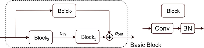
Figure 2. A basic block in ResNets used in this paper. The shortcut consists of one block with convolutional and batch-normalization layers, while the main stream has two blocks. ResNets are constructed as a cascading of several basic blocks of various sizes.
3. Experimental Results
The spirit of the following experiments is to show when and how the margin bound above could be used to numerically predict the tendency of generalization or test error along the training path. We are going to show examples of both success and failure.
3.1. Networks and Datasets
The networks and datasets used in the experiments are introduced in brief here. For the network, our illustration, Example 1.1, is based on a simple convolutional neural network whose architecture is shown in Figure 3 (more details in Figure A1 in Appendix), called basic CNN(c), here with c channels that will be specified in different experiments below. It essentially has five convolutional layers of c channels at each one, and this is followed by batch normalization and ReLU as well as a fully connected layer in the end. Furthermore, we consider various popular networks in applications, including AlexNet [24], VGG-16 [25], and ResNet-18 [26]. For the dataset, we consider CIFAR10, CIFAR100 [27], and Mini-ImageNet [28].
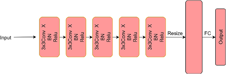
Figure 3. Illustration of the architecture of basic CNN.
3.2. Success: Similar Phase Transitions in Training and Test Margin Dynamics
In this section, we show that when the expressive power of models are comparable to data complexity, the dynamics of training margin distributions and that of test margin distributions share similar phase transitions, which enables us to predict generalization (test) error utilizing the theorems in this paper. In this experiment, we are going to demonstrate when there is a nearly monotone relationship between training margin error and test margin error such that Theorem 1 and Theorem 2 can be applied to predict the tendency of generalization (test) error.
Let us first consider training a basic CNN(50) on CIFAR10 dataset with and without random noise. The relations between test error and training margin error with γ = 9.8, inverse quantile margin with q = 0.6 are shown in Figure 4. In this simple example, where the network is small and the dataset is simple, the bounds (9) and (12) show a good prediction power: they stop either near the epoch of sufficient training without noise (Left, original data) or before an overfitting occurs with noise (Right, 10% label corrupted).
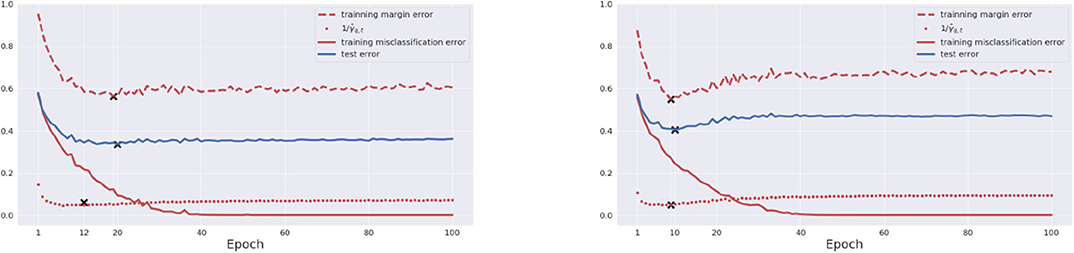
Figure 4. Success examples. Net structure: basic CNN (50). Dataset: Original CIFAR10 (Left) and CIFAR10 with 10% label corrupted (Right). In each figure, we show training error (red solid), training margin error γ = 9.8 (red dash), inverse quantile margin (red dotted) with q = 0.6, and generalization error (blue solid). The marker “x” in each curve indicates the global minimum along epoch 1, …, T. Both training margin error and inverse quantile margin successfully predict the tendency of generalization error.
Why does it work in this case? Here are some detailed explanations on its mechanism. The training margin error () and the inverse quantile margin () are both closely related to the dynamics of training margin distributions. Figure 1B actually shows that the dynamics of training margin distributions undergo a phase transition: while the low margins have a monotonic increase, the high or large margins undergo a phase transition from increase to decrease, which is indicated by the red arrows. Therefore different choices of γ for the linear bounds (9) [a parallel argument holds for q in (12)] will have different effects. In fact, the training margin error with a small γ is close to the training error, while that with a large γ is close to test error. Figure 5 shows such a relation using rank correlations (in terms of Spearman-ρ and Kendall-τ1) between training margin errors (or inverse quantile margins) and training errors, as well as training margin errors (or inverse quantile margins) and test errors, for each γ (or q, respectively). In these plots, we see that the dynamics of large margins have a trend that is similar to the test errors, while small margins are close to training errors in rank correlations. For a good prediction, one should thus choose a large enough γ = 9.8 (or q = 6.8, respectively) at the peak point of the rank correlation curve between training margins and test errors. Under these conditions, the epoch when the phase transition above happens is featured with a cross-over in dynamics of training margin distributions in Figure 1B and exists near the optima of the training margin error curve.
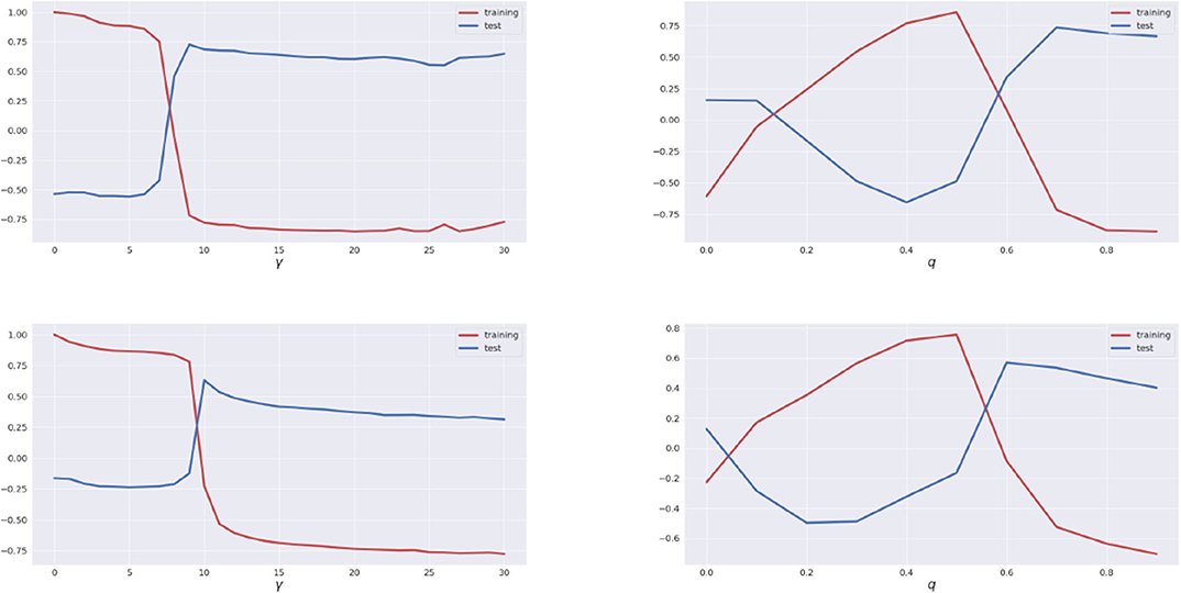
Figure 5. Spearman's ρ and Kendall's τ rank correlations between training (or quantile) margins and training errors, as well as training (or quantile) margins and test errors, at different γ (or q, respectively). Net structure: Basic CNN(50). Dataset: CIFAR10. Top: Spearman's ρ rank correlation. Bottom: Kendall's τ rank correlation. (Left) Blue curves show rank correlations between training margin error and test (generalization) error, while Red curves show that between the training margin error and training error, at different γ. (Right) Blue curves show rank correlations between inverse quantile margin and test error, and Red curves show the same between inverse quantile margin and training error at different q. Both Spearman's ρ and Kendall's τ show qualitatively the same phenomenon that dynamics of large margins are closely related to the test errors in the sense that they have similar trends marked by large rank correlations. On the other hand, small margins are close to training errors in trend.
Although both the training margin error () and the inverse quantile margin () can be used here to successfully predict the trend of test (generalization) error, the latter can be more powerful in our studies. In fact, dynamics of the inverse quantile margins can adaptively select γt for each ft without access to the complexity term. Unlike merely looking at the training margin error with a fixed γ, the quantile margin bound (12) in Theorem 2 shows a stronger prediction power than (10) and is even able to capture more local optima. In Figure 6, the test error curve has two valleys corresponding to a local optimum and a global optimum, and the quantile margin curve with q = 0.95 successfully identifies both. However, if we consider the dynamics of training margin errors, it is rarely possible to recover the two valleys at the same time since their critical thresholds γt1 and γt2 are different. Another example of ResNet-18 is given in Figure A2 in the Appendix.
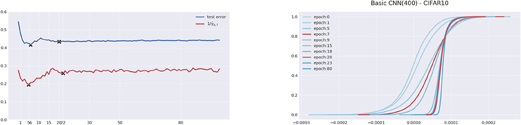
Figure 6. Inverse quantile margin. Net structure: CNN(400). Dataset: CIFAR10 with 10% of the label corrupted. (Left) The dynamics of test error (blue) and inverse quantile margin with q = 0.95 (red). Two local minima are marked by “x” in each curve. (Right) Dynamics of training margin distributions, where two distributions in red color correspond to when the two local minima occur. The inverse quantile margin successfully captures two local minima of test error.
In a summary, when training and test margin dynamics share similar phase transitions, both theorems we developed can be used to predict test (generalization) error via normalized training margins, even leaving us with the data-dependent early stopping rule to avoid overfitting when data is noisy. However, below we shall see a different scenario when training and test margin dynamics are of distinct phase transitions, such a prediction fails as Breiman's dilemma.
3.3. Failure: Distinct Phase Transitions in Margin Dynamics and Breiman's Dilemma
In this section, when model complexity arbitrarily increases to be over-expressive against the dataset, the training margins can be monotonically improved, while high test margin dynamics undergo a distinct phase transition of decrease-increase. In this case, the prediction power of training-margin-based bounds is lost and overfitting may set in. This exhibits Breiman's dilemma in neural networks.
We conduct three sets of experiments in the following.
3.3.1. Experiment I: Basic CNNs on CIFAR10
In the first experiment shown in Figure 7, we fix the dataset to be CIFAR10 with 10% of labels randomly permuted and gradually increase the channels from basic CNN(50) to CNN(400). For CNN(50) [#(parameters) is 92,610] and CNN(100) [#(parameters) is 365,210], both training margin dynamics and test margin dynamics share a similar phase transition during training: small margins are monotonically improved while large margins are firstly improved then dropped afterwards. The last row in Figure 7 shows the heatmaps as Spearman-ρ rank correlations between these two dynamics drawn in γ1-γ2 plane. The block diagonal structures in the rank correlation heatmaps illustrates such a similarity in phase transitions. To be specific, small (or large) margins in both training margins and test margins share high-level rank correlations marked by diagonal blocks in light color, while the difference between small and large margins are marked by off-diagonal blocks in dark color. Particularly at γ1 = 0, the test (generalization) error dynamics can be predicted using large training margins, as their rank correlations are high.
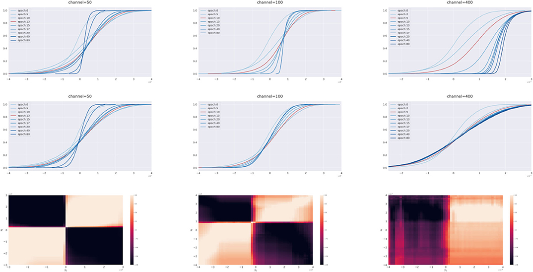
Figure 7. Breiman's Dilemma I: comparisons between dynamics of test margin distributions and training margin distributions. Net structure: Basic CNN(50) (Left), Basic CNN(100) (Middle), and Basic CNN(400) (Right). Dataset: CIFAR10 with 10 percent labels corrupted. First row: evolutions of training margin distributions. Second row: evolutions of test margin distributions. Third row: heatmaps are Spearman-ρ rank correlation coefficients between dynamics of training margin error () and dynamics of test margin error () drawn on the (γ1, γ2) plane. CNN(50) and CNN(100) share similar phase transitions in training and test margin dynamics while CNN(400) does not. When model becomes over-representative to the dataset, training margins can be monotonically improved, whereas test margins cannot be, as they lose their predictability.
However, as the channel number increases to CNN(400) [#(parameters) is 5,780,810], the dynamics of the training margin distributions becomes a monotone improvement without the phase transition above. This phenomenon is not a surprise, as, with a strong representation power, the whole training margin distribution can be monotonically improved without sacrificing the large margins. On the other hand, the generalization or test error cannot be monotonically improved. The heatmap of rank correlations between training and test margin dynamics thus exhibits such a distinction in phase transitions by changing the block diagonal structure above to double column blocks for CNN(400). In particular, for γ1 ≤ 0, test margin dynamics have low rank correlations with all training margin dynamics as they are of different phase transitions in evolutions. As a result, one cannot predict test error at γ = 0 using training margin dynamics.
3.3.2. Experiment II: CNN(400) and ResNet-18 on CIFAR100 and Mini-ImageNet
In the second experiment shown in Figure 8, we compare the normalized margin dynamics of training CNN(400) and ResNet-18 on two different datasets, CIFAR100 and Mini-ImageNet. CIFAR100 is more complex than CIFAR10 but less complex than Mini-ImageNet. It shows that (a) CNN(400) does not have an over-expressive power on CIFAR100, whose normalized training margin dynamics exhibits a phase transition—a sacrifice of large margins to improve small margins during training; it also shows that (b) ResNet-18 does have an over-expressive power on CIFAR100 by exhibiting a monotone improvement on training margins but loses such a power in Mini-ImageNet with phase transitions of training margin dynamics.
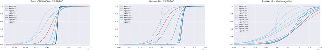
Figure 8. Breiman's Dilemma II. Net structure: Basic CNN(400) (Left), ResNet-18 (Middle, Right). Dataset: CIFAR100 (Left, Middle), Mini-ImageNet (Right) with 10% of the labels corrupted. With a fixed network structure, we further explore how the complexity of dataset influences the margin dynamics. Taking ResNet-18 as an example, margin dynamics on CIFAR100 doesn't have any cross-over (phase transition), but on Mini-Imagenet a cross-over occurs.
From this experiment, one can see that simply counting the number of parameters and samples cannot tell us if the model and data complexities are over-representative or comparable. Instead, phase transitions of margin dynamics provide us a tool to investigate their relationship. CNN(400) (5.8 M parameters) has a power that is too expressive for the simplest CIFAR10 dataset such that the training margins can be monotonically improved during training; but CNN(400)'s expressive power seems comparable to the more complex CIFAR100. Similarly, the more complex model ResNet-18 (11 M parameters) has a too much expressive power for CIFAR100 but seems comparable to Mini-ImageNet.
3.3.3. Comparisons of Basic CNNs, AlexNet, VGG16, and ResNet-18 in CIFAR10/100 and Mini-ImageNet
In this part, we collect comparisons of various networks on the CIFAR10/100 and Mini-ImageNet dataset. Figure 9 shows both success and failure cases with different networks and datasets. In particular, the predictability of generalization error based on Theorem 1 and Theorem 2 can be rapidly observed on the third column of Figure 9, the heatmaps of rank correlations between training margin dynamics and test margin dynamics. On one hand, one can use the training margins to predict the test error as shown in the first column of Figure 9. In these cases, model complexity is comparable to data complexity such that the training margin dynamics share similar phase transitions with test margin dynamics, indicated by block diagonal structures in rank correlations [e.g., CNN(100)—CIFAR10, AlexNet—CIFAR100, AlexNet—MiniImageNet, VGG16—MiniImageNet, and ResNet-18—MiniImageNet]. On the other hand, such a prediction fails when models become over-expressive against datasets such that the training margin dynamics undergo different phase transitions to test margin dynamics, indicated by the loss of block diagonal structures in rank correlations [e.g., CNN(400)—CIFAR10, ResNet-18—CIFAR100, and VGG16—CIFAR100].
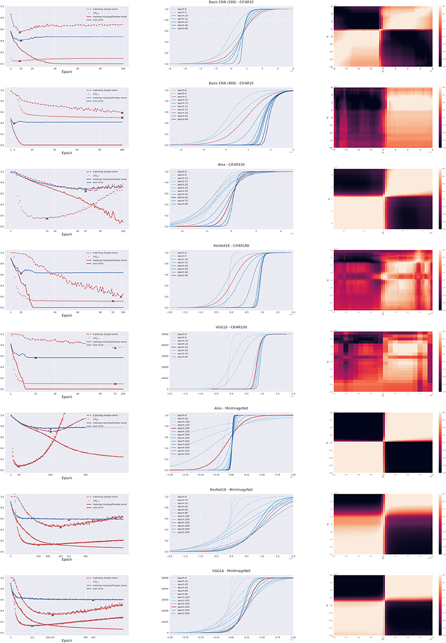
Figure 9. Comparisons of Basic CNNs, AlexNet, VGG16, and ResNet-18 in CIFAR10/100 and Mini-ImageNet. The dataset and network in use are marked in titles of middle pictures in each row. (Left) Curves of training error, generalization error, training margin error, and inverse quantile margin. (Middle) Dynamics of training margin distributions. (Right) heatmaps are Spearman-ρ rank correlation coefficients between dynamics of training margin error () and dynamics of test margin error () drawn on the (γ1, γ2) plane.
As we have shown, phase transitions of margin dynamics play a central role in characterizing the trade-off between model expressive power and data complexity, hence the predictability of generalization error by our theorems. If one tries hard to improve training margins by arbitrarily increasing the model complexity, the training margin distributions can be monotonically enlarged but may lead to overfitting. This phenomenon is not unfamiliar to us, since Breiman has pointed out that the improvement of training margins is not enough to guarantee a small generalization or test error in the boosting type algorithms [17]. We find the same phenomenon ubiquitous in deep neural networks. In this paper, the inspection of the trade-off between expressive power of models and complexity of data via phase transitions of margin dynamics provides us with a new perspective to study the Breiman's dilemma in applications.
3.4. Discussion: Effluence of Normalization Factor Estimates
In the end, it is worth mentioning that different choices of the normalization factor estimation may affect the range of predictability but may still exhibit Breiman's dilemma. In all experiments above, the normalization factor is estimated via the ℓ1-based estimate in Proposition 2 in section 2.4. One could also use power iteration [14] to present a more precise estimation on spectral norm. Usually the ℓ1-based estimates lead to a coarser upper bound than the power iterations, see Figure 10. It is a fact that, in training margin dynamics, large margins are typically improved at a slower speed than small margins. A more accurate estimation of spectral norm with faster increases in training may thus bring with it cross-overs (or phase transitions) in large training margins and extend the range of predictability. Breiman's dilemma, however, still persists when the balance between model representation power and dataset complexity is broken as model complexity arbitrarily grows.
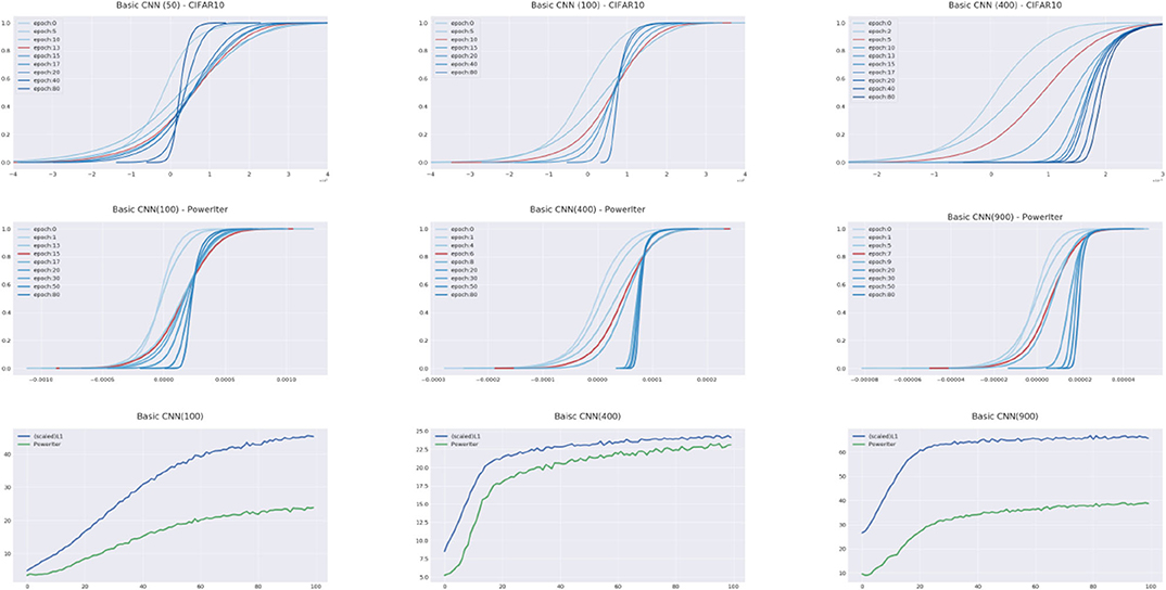
Figure 10. Comparisons on normalization factor estimates by power iteration and the ℓ1-based estimate. Dataset: CIFAR10 with 10 percent corrupted. Net structure: Basic CNN with channels 50 (Top, Left), 100 (Top, Middle), 400 (Top Right), 200 (Middle, Left), 600 (Middle, Middle), and 900 (Middle, Right). In the top row, the spectral norm in Lf is estimated via the ℓ1-based estimate method and in the middle row, the spectral norm is estimated by power iteration. Bottom pictures show the estimates of Lf by power iterations (in green color) and by the ℓ1-based estimate method (in blue color), respectively. The curves of Lf estimates are rescaled for visualization since a fixed scaling factor and training does not influence the occurrence of cross-overs or phase transitions. Note that the original ℓ1-based estimates are of order 1e + 17, 1e + 19, and 1e + 21 (100 channels, 400 channels, and 900 channels, respectively), and the power iteration estimates are of 1e + 3, 1e + 3, and 1e + 3 (100 channels, 400 channels, and 900 channels, respectively). As shown above, a more accurate estimation of spectral norm may extend the range of predictability but eventually faces Breiman's dilemma if the model representation power grows too much against the dataset complexity.
4. Conclusion and Future Directions
In this paper, we show that Breiman's dilemma is ubiquitous in deep learning, in addition to previous studies on Boosting algorithms. We further show that Breiman's dilemma is closely related to the trade-off between the expressive power of models and the complexity of data. Large margins within training data do not guarantee a good control on model complexity. Instead, we have shown that phase transitions in dynamics of normalized margin distributions are able to reflect the trade-off between model expressiveness and data complexity. In particular, if high or large training margin distributions undergo decrease-increase phase transitions during training, which is similar to that of test margins, model expressiveness is comparable to data complexity and normalized training margin-based generalization bounds has the prediction power in capturing possible overfitting. We have shown two theorems derived from normalized Rademacher complexity bounds can be used to quantitatively capture a data-driven early stopping rule to prevent overfitting. However, if the training margin distributions, both high and low parts, undergo a uniform increase during training, the model exhibits over expressiveness with respect to the data, and the margin theory above fails. Such phase transitions of margin evolutions may reflect the degree-of-freedom of models with respect to data, which measures the sensitivity of model prediction over data response. Roughly speaking, an increase-decrease phase transition in high margin distributions together with a decrease in low margin distributions, indicates the degree-of-freedom of models is relatively smaller than the data complexity where one has to sacrifice the high margin predictions to improve the low margin predictions. In contrast, a uniform increase of margins over all sample suggests that the degree-of-freedom of models are larger than the data complexity. A detailed study still remains to be made for the future of designing a data-driven early stopping rule and degree-of-freedom for models through the monitoring of the margin dynamics.
Data Availability Statement
Publicly available datasets were analyzed in this study. This data can be found at: Cifar dataset: https://www.cs.toronto.edu/~kriz/cifar.html; imageNet: http://www.image-net.org/.
Author Contributions
WZ proved the theorems, conducted some experiments, and wrote the paper. YH carried out major experiments. YY designed the project and wrote the paper. All authors contributed to the article and approved the submitted version.
Funding
The research was supported in part by the Hong Kong Research Grant Council (HKRGC) grant 16303817, Innovation and Technology Fund (ITF) UIM/390, the National Natural Science Foundation of China (No. 61370004, 11421110001), as well as awards from the Tencent AI Lab and Si Family Foundation.
Conflict of Interest
The authors declare that the research was conducted in the absence of any commercial or financial relationships that could be construed as a potential conflict of interest.
Acknowledgments
We thank Tommy Poggio, Peter Bartlett, and Xiuyuan Cheng for helpful discussions.
Supplementary Material
The Supplementary Material for this article can be found online at: https://www.frontiersin.org/articles/10.3389/fams.2020.575073/full#supplementary-material
Footnotes
1. ^The Spearman's ρ and Kendall's τ rank correlation coefficients measure how two variables are correlated up to a monotone transformation, and a larger correlation means a closer tendency.
References
1. Novikoff ABJ. On convergence proofs on perceptrons. In: Proceedings of the Symposium on the Mathematical Theory of Automata, Vol. 12. New York, NY (1962). p. 615–22.
4. Bartlett PL. For valid generalization the size of the weights is more important than the size of the network. In: Mozer MC, Jordan MI, Petsche T, Editors. Advances in Neural Information Processing Systems 9. Cambridge, MA: MIT Press (1997). p. 134–40.
5. Bartlett PL. The sample complexity of pattern classification with neural networks: the size of the weights is more important than the size of the network. IEEE Trans Inform Theory. (1998) 44:525–36.
6. Freund Y, Schapire RE. A decision-theoretic generalization of on-line learning and an application to boosting. J Comput Syst Sci. (1997) 55:119.
7. Schapire RE, Freund Y, Bartlett P, Lee WS. Boosting the margin: a new explanation for the effectiveness of voting methods. Ann. Stat. (1998) 26:1651–86.
8. Koltchinskii V, Panchenko D. Empirical margin distributions and bounding the generalization error of combined classifiers. Ann Stat. (2002) 30:1–50. doi: 10.1214/AOS/1015362183
9. Bühlmann P, Yu B. Boosting with the l2-loss: Regression and classification. J Am Stat Assoc. (2002). 98:324–40. doi: 10.1198/016214503000125
10. Zhang T, Yu B. Boosting with early stopping: Convergence and consistency. Ann Stat. (2005) 33:1538–79. doi: 10.1214/009053605000000255
11. Yao Y, Rosasco L, Caponnetto A. On early stopping in gradient descent learning. Construct Approx. (2007) 26:289–315. doi: 10.1007/s00365-006-0663-2
12. Zhang C, Bengio S, Hardt M, Recht B, Vinyals O. Understanding deep learning requires rethinking generalization. In: International Conference on Learning Representations. Toulon (2017).
13. Bartlett P, Foster DJ, Telgarsky M. Spectrally-normalized margin bounds for neural networks. In: The 31st Conference on Neural Information Processing Systems (NIPS). Long Beach, CA (2017).
14. Miyato T, Kataoka T, Koyama M, Yoshida Y. Spectral normalization for generative adversarial networks. In: The 6th International Conference on Learning Representations (ICLR) (2018).
15. Neyshabur B, Bhojanapalli S, Srebro N. A pac-bayesian approach to spectrally-normalized margin bounds for neural networks. In: The 6th International Conference on Learning Representations (ICLR). Vancouver, BC (2018).
16. Liao Q, Miranda B, Banburski A, Hidary J, Poggio T. A surprising linear relationship predicts test performance in deep networks. MIT CBMM memo (2018).
18. Cortes C, Mohri M, Rostamizadeh A. Multi-class classification with maximum margin multiple kernel. In: International Conference on Machine Learning. Atlanta (2013). p. 46–54.
19. Kuznetsov V, Mohri M, Syed U. Rademacher complexity margin bounds for learning with a large number of classes. In: ICML Workshop on Extreme Classification: Learning With a Very Large Number of Labels. Lille (2015).
20. Telgarsky M. Margins, shrinkage, and boosting. In: Proceedings of the 30th International Conference on Machine Learning (ICML). Atlanta (2013).
21. Soudry D, Hoffer E, Srebro N. The implicit bias of gradient descent on separable data. In: The 6th International Conference on Learning Representations (ICLR). Vancouver, BC (2018).
22. Bogachev VI. Measure Theory. Vol. 1. Berlin/Heidelberg: Springer Science & Business Media (2007).
23. Golub GH, Van der Vorst HA. Eigenvalue computation in the 20th century. In: Numerical Analysis: Historical Developments in the 20th Century. Elsevier (2001). p. 209–39.
24. Krizhevsky A, Sutskever I, Hinton GE. Imagenet classification with deep convolutional neural networks. In: Advances in Neural Information Processing Systems (NIPS). Lake Tahoe (2012). p. 1097–105.
25. Simonyan K, Zisserman A. Very deep convolutional networks for large-scale 1458 image recognition. In: International Conference on Learning Representations. San Diego, CA (2015).
26. He K, Zhang X, Ren S, Sun J. Deep residual learning for image recognition. In: Proceedings of the IEEE Conference on Computer Vision and Pattern Recognition (CVPR). Las Vegas (2016). p. 770–8.
27. Krizhevsky A, Hinton G. Learning Multiple Layers of Features From Tiny Images. Toronto, ON: Technical report, Citeseer (2009).
Keywords: generalization ability, Rademacher complexity, margin theory, Breiman's dilemma, phase transitions
Citation: Zhu W, Huang Y and Yao Y (2020) Rethinking Breiman's Dilemma in Neural Networks: Phase Transitions of Margin Dynamics. Front. Appl. Math. Stat. 6:575073. doi: 10.3389/fams.2020.575073
Received: 22 June 2020; Accepted: 17 August 2020;
Published: 30 October 2020.
Edited by:
Xiaoming Huo, Georgia Institute of Technology, United StatesReviewed by:
Jinshan Zeng, Jiangxi Normal University, ChinaYuling Jiao, Zhongnan University of Economics and Law, China
Copyright © 2020 Zhu, Huang and Yao. This is an open-access article distributed under the terms of the Creative Commons Attribution License (CC BY). The use, distribution or reproduction in other forums is permitted, provided the original author(s) and the copyright owner(s) are credited and that the original publication in this journal is cited, in accordance with accepted academic practice. No use, distribution or reproduction is permitted which does not comply with these terms.
*Correspondence: Yuan Yao, eXVhbnlAdXN0Lmhr