On the Relation Between Smooth Variable Structure and Adaptive Kalman Filter

1. Introduction

State estimation plays an important role in the field of control. System states are required for the calculation of state feedback controllers, exact input-/output linearizations, equivalent control, backstepping control, etc. Noise reduction of signals is desirable to improve performance of sliding mode approaches under real conditions. Combined input-state estimation is useful for the estimation and rejection of unknown exogenuous inputs. Additionally, robust model-based fault detection and localization approaches can be designed based on filters.

Related to linear systems minimum variance unbiased [1, 2] and augmented state filters [3, 4] can be used for combined input-state estimation. In case of known uncertainty bounds robust Kalman filters [5] can improve state estimation of uncertain linear systems. In the field of $H_{\infty }$ filtering robustness of the state estimation may be improved by minimizing the effect of worst possible energy-bounded disturbances on the estimation error [6]. Multiple-model approaches [7] are a powerful tool for state estimation of uncertain systems. Combining them with the particle filter allows state estimation of nonlinear systems [8].

The smooth variable structure filter (SVSF) introduced in Ref. 9 is an approach for state estimation of uncertain nonlinear systems. Several applications of SVSF can be found in the literature. The filter has been applied to estimate the states and parameters of an uncertain linear hydraulic system in Ref. 9. A multiple-model approach has been formulated for fault detection e.g., leakage of the hydraulic system [10]. The state of charge and state of health of batteries is estimated in Refs. 11 and 12. A multiple-model approach has been applied for target tracking in Ref. 13 and a SVSF based probabilistic data association (PDA) approach has been proposed for tracking in cluttered environment [14]. For multiple object tracking a SVSF based joint-PDA approach has been developed [15]. Online multiple vehicle tracking on real road scenarios has been investigated in Ref. 16. Several SVSF based simultaneous localization and mapping algorithms have been proposed e.g., Refs. 17–19. Training of neural networks based on SVSF and classification of engine faults has been studied in Ref. 20. Dual estimation of states and model parameters has been considered in Ref. 21. The estimation strategy works as follows. The bi-section method, the shooting method, and SVSF are combined. The bi-section and shooting method are applied to determine best-fitting model parameter combinations. The obtained model is used by SVSF to estimate the system states. To apply the bi-section method the measurement signals are divided into segments in which the model parameters remain nearly constant. In comparison to the Kalman filter the SVSF approach facilitates detection of these segments based on an evaluation of chattering process.

As described in Ref. 9 the SVSF approach uses a switching gain to drive the estimated state trajectory into a region around the true state trajectory called existence subspace. Due to measurement noise chattering occurs in the existence subspace. By introducing a boundary layer, similar to the saturation function approach of sliding mode control, the high frequency switching in the existence subspace can be attenuated. The claimed advantage of SVSF approach is that if the boundary layer is not used, the filter guarantees to reach the existence subspace for sure although an imprecise system model may be used. It is shown in Ref. 22 that in case of not using the boundary layer the estimations of the filter converge to the measurements, which guarantees the estimation error to be bounded. However, this is a trivial result because if the estimations are equal to the measurements and every state is measured, than the filter is not required. If the boundary layer is used, the estimations diverge from the noisy measurements and estimation performance improves. Unfortunately, it has never been proven that the SVSF with boundary layer has bounded estimation error in case of using an imprecise model.

As already mentioned a serious limitation of the SVSF approach is that all system states have to be measured. Additionally, the measurement model is required to be linear. However, related to tracking a linear measurement model may be achievd by applying a measurement conversion [23] and measurements of the vehicle velocities could also be derived from measured positions.

Another problem of SVSF results from the dependency of the estimation performance on the width of the introduced smoothing boundary layer. In Ref. 24 an estimation error model for the SVSF is proposed and in Ref. 25 the estimation error is minimized according to the smoothing boundary layer width. A maximum a posteriori estimation of the noise statistics of the error model is discused in Ref. 26. However, the derived estimation error model and the related approaches require the system to be linear and precisely known which contradicts the idea of robustness.

In our previous publication [22] a new tuning parameter for the SVSF approach was introduced to achieve online optimization of the estimation performance. In this paper the relation between the SVSF approach and the Kalman filter is studied. An adaptive Kalman filter is obtained from the SVSF approach by replacing the original filter gain. The estimation performance of SVSF and the adaptive filter variant is compared with one another. Therefore, a parameter optimization scheme is proposed. In the simulation results the adaptive Kalman filter shows superior performance compared to the original SVSF approach.

The paper is organized as follows. In Section 2 the preliminaries and the original SVSF approach are discussed. In Section 3 the relation of SVSF and Kalman filter is studied. Parameter optimization of the Kalman filter leading to an adaptive filtering approach is considered in Section 4. The stability of the adaptive filter is studied in Section 5. A performance evaluation of SVSF and adaptive Kalman filter is provided in Section 6.

Notations. An overview of the notations used within the paper is given in Table 1.

TABLE 1

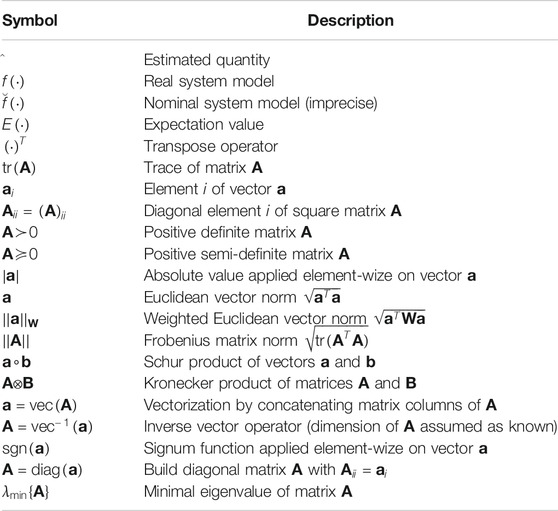
TABLE 1. Nomenclature.

2. Problem Formulation and Previous Work

Consider the dynamics of a nonlinear system to be exactly described by the discrete-time model

${\mathbf{x}}_{k+1}=f_k\left({\mathbf{x}}_k,{\mathbf{u}}_k\right),(1)$

${\mathbf{y}}_k={\mathbf{x}}_k+{\mathbf{r}}_k,(2)$

with states ${\mathbf{x}}_k\in {\mathrm{ℝ}}^n$, inputs ${\mathbf{u}}_k\in {\mathrm{ℝ}}^m$, and outputs ${\mathbf{y}}_k\in {\mathrm{ℝ}}^n$. The process ${\mathbf{r}}_k\in {\mathrm{ℝ}}^n$ is assumed to be a white noise process with independent samples described by the covariances $E\left({\mathbf{r}}_k{\mathbf{r}}_k^T\right)=\mathbf{R}\succ 0$, and $E\left({\mathbf{r}}_i{\mathbf{r}}_j^T\right)=0$, for $i\ne j$, and the mean $E\left({\mathbf{r}}_k\right)=0$. The measurement model Eq. 2 can be obtained from any model of the form ${\tilde{\mathbf{y}}}_k={\mathbf{H}}_k{\mathbf{x}}_k+{\tilde{\mathbf{r}}}_k$ as the considered SVSF approach requires ${\mathbf{H}}_k$ to be invertible [9]. Consider ${\breve{f}}_k$ to be a nominal description of system $\left(\mathrm{1,2}\right)$, which may differ from the true behavior. According to Ref. 9 an estimation $\widehat{\mathbf{x}}$ of the system states $\mathbf{x}$ can be obtained using the SVSF algorithm

${\mathbf{e}}_{y_{k|k}}={\mathbf{y}}_k-{\widehat{\mathbf{x}}}_{k|k},(3)$

${\widehat{\mathbf{x}}}_{k+1|k}=\breve{f}\left({\widehat{\mathbf{x}}}_{k|k},{\mathbf{u}}_k\right),(4)$

${\mathbf{e}}_{y_{k+1|k}}={\mathbf{y}}_{k+1}-{\widehat{\mathbf{x}}}_{k+1|k},(5)$

${\mathbf{M}}_{k+1}=\left(\left|{\mathbf{e}}_{y_{k+1|k}}\left|+\mathbf{\Phi }\right|{\mathbf{e}}_{y_{k|k}}\right|\right)\circ \text{sat}\left({\mathbf{e}}_{y_{k+1|k}},\mathbf{\Psi }\right),(6)$

${\widehat{\mathbf{x}}}_{k+1|k+1}={\widehat{\mathbf{x}}}_{k+1|k}+{\mathbf{M}}_{k+1},(7)$

where the operator “$\circ$” denotes the Schur product, $\mathbf{\Phi }$ and $\mathbf{\Psi }$ are diagonal matrices with ${\mathbf{\Phi }}_{ii}$, ${\mathbf{\Psi }}_{ii}$ denoting the ith diagonal element, and the ith element of vector $\text{sat}\left({\mathbf{e}}_{y_{k+1|k}},\mathbf{\Psi }\right)$ is defined as

$\text{sat}{\left(\mathbf{a},\mathbf{A}\right)}_i=\{\begin{array}{ll}1\hfill & \text{for }\frac{{\mathbf{a}}_i}{{\mathbf{A}}_{ii}}>1,\hfill \\ -1\hfill & \text{for }\frac{{\mathbf{a}}_i}{{\mathbf{A}}_{ii}}<-1,\hfill \\ \frac{{\mathbf{a}}_i}{{\mathbf{A}}_{ii}}\hfill & \text{for}-1\le \frac{{\mathbf{a}}_i}{{\mathbf{A}}_{ii}}\le 1,\hfill \end{array}(8)$

where $i\in \left\{\mathrm{1,2},\dots ,n\right\}$. According to Ref. 22 the SVSF algorithm (Eqs 3–7) reduces to

${\widehat{\mathbf{x}}}_{k+1|k}={\breve{f}}_k\left({\widehat{\mathbf{x}}}_{k|k},{\mathbf{u}}_k\right),(9)$

${\mathbf{e}}_{y_{k+1|k}}={\mathbf{y}}_{k+1}-{\widehat{\mathbf{x}}}_{k+1|k},(10)$

${\widehat{\mathbf{x}}}_{k+1|k+1}={\mathbf{y}}_{k+1}-{\tilde{\mathbf{M}}}_{k+1}{\mathbf{e}}_{y_{k+1|k}},(11)$

${\tilde{\mathbf{M}}}_{k+1}=\text{diag}\left({\mathbf{I}}_{n\times 1}-\left|\text{sat}\left({\mathbf{e}}_{y_{k+1|k}},\mathbf{\Psi }\right)\right|\right),(12)$

in case of $\mathbf{\Phi }=0_{n\times n}$.

Theorem 1 of Ref. 9 proves that the output estimation error ${\mathbf{e}}_{y_{k|k}}$ of algorithm (Eqs 3–7) approaches zero if instead of the gain ${\mathbf{M}}_{k+1}$ the gain ${\mathbf{M}}_{k+1}^{\mathrm{\star }}=\left(\left|{\mathbf{e}}_{y_{k+1|k}}\left|+\mathbf{\Phi }\right|{\mathbf{e}}_{y_{k|k}}\right|\right)\circ \text{sgn}\left({\mathbf{e}}_{y_{k+1|k}}\right)$ is used. As a consequence the estimations of the filter equal the measurements, i.e., ${\mathbf{e}}_{y_{k|k}}={\mathbf{y}}_k-{\widehat{\mathbf{x}}}_{k|k}=0$. This is a trivial result as all states are required to be measured. So one might just use the measurements instead of the filter estimates. The estimations of the filter diverge from the measurements and estimation performance improves if a boundary layer is introduced and gain ${\mathbf{M}}_{k+1}^{\mathrm{\star }}$ is replaced by ${\mathbf{M}}_{k+1}$. However, it has neither been proven that algorithm (Eqs 3–7) with gain ${\mathbf{M}}_{k+1}$ has a bounded estimation error, nor it has been shown that the introduced boundary layer minimizes the squared estimation error or some other performance criterion.

3. Relation Between Smooth Variable Structure and Kalman Filter

In this section the stochastic gain ${\tilde{\mathbf{M}}}_{k+1}$ of SVSF approach is replaced by a deterministic but yet undefined gain ${\mathbf{K}}_{k+1}$. Using the deterministic gain the estimation error covariance matrix of the filter is determined. By minimizing the mean squared estimation error (MSE) the deterministic gain ${\mathbf{K}}_{k+1}$ becomes the specific optimal one ${\mathbf{K}}_{k+1}^{\text{opt}}$. Replacing the original gain ${\tilde{\mathbf{M}}}_{k+1}$ of SVSF by the optimal one ${\mathbf{K}}_{k+1}^{\text{opt}}$ gives a direct link to the Kalman filter.

From Eqs 1, 2, and 9–12 it follows that the state estimation error and the output estimation error can be determined as

${\mathbf{e}}_{x_{k+1|k+1}}={\mathbf{x}}_{k+1}-{\widehat{\mathbf{x}}}_{k+1|k+1}={\mathbf{K}}_{k+1}{\mathbf{e}}_{y_{k+1|k}}-{\mathbf{r}}_{k+1},(13)$

and

${\mathbf{e}}_{y_{k+1|k}}={\mathbf{y}}_{k+1}-{\widehat{\mathbf{x}}}_{k+1|k}={\mathbf{e}}_{x_{k+1|k}}+{\mathbf{r}}_{k+1},(14)$

where ${\mathbf{K}}_{k+1}$ is a deterministic but yet undefined gain. To derive the optimal gain that minimizes the MSE an expression of the a posteriori error covariance dependent on ${\mathbf{K}}_{k+1}$ is required to be derived. However, first of all the calculation of the output error covariance is considered. Inserting Eq. 14 into the definition of the output error covariance ${\mathbf{S}}_{k+1}=E\left({\mathbf{e}}_{y_{k+1|k}}{\mathbf{e}}_{y_{k+1|k}}^T\right)$ gives

${\mathbf{S}}_{k+1}=E\left(\left({\mathbf{e}}_{x_{k+1|k}}+{\mathbf{r}}_{k+1}\right){\left({\mathbf{e}}_{x_{k+1|k}}+{\mathbf{r}}_{k+1}\right)}^T\right).(15)$

Expanding Eq. 15 and considering the definition of the a priori estimation error covariance ${\mathbf{P}}_{k+1|k}=E\left({\mathbf{e}}_{x_{k+1|k}}{\mathbf{e}}_{x_{k+1|k}}^T\right)$ and the stationary measurement noise covariance $\mathbf{R}=E\left({\mathbf{r}}_{k+1}{\mathbf{r}}_{k+1}^T\right)$ yields

${\mathbf{S}}_{k+1}={\mathbf{P}}_{k+1|k}+\mathbf{R}+E\left({\mathbf{r}}_{k+1}{\mathbf{e}}_{x_{k+1|k}}^T\right)+E\left({\mathbf{e}}_{x_{k+1|k}}{\mathbf{r}}_{k+1}^T\right).(16)$

The value of the remaining expectations in Eq. 16 is studied as follows. First of all the a priori estimation error ${\mathbf{e}}_{x_{k+1|k}}$ is known to directly depend on the noise realizations ${\mathbf{r}}_j$ with $j\in \left\{\mathrm{0,1},\dots ,k\right\}$ but not on the realization ${\mathbf{r}}_{k+1}$. In addition ${\mathbf{r}}_j$ with $j\in \left\{\mathrm{0,1},\dots ,k\right\}$ and ${\mathbf{r}}_{k+1}$ are independent of each other due to the independent white noise assumption. Finally, ${\mathbf{r}}_{k+1}$ can not have any effect on ${\mathbf{e}}_{x_{k+1|k}}$ and both random variables are stochastically independent. It follows $E\left({\mathbf{r}}_{k+1}{\mathbf{e}}_{x_{k+1|k}}^T\right)=E\left({\mathbf{r}}_{k+1}\right)E\left({\mathbf{e}}_{x_{k+1|k}}^T\right)$ and $E\left({\mathbf{e}}_{x_{k+1|k}}{\mathbf{r}}_{k+1}^T\right)=E\left({\mathbf{e}}_{x_{k+1|k}}\right)E\left({\mathbf{r}}_{k+1}^T\right)$. From the zero-mean assumption of the noise i.e., $E\left({\mathbf{r}}_k\right)=0$ it follows

${\mathbf{S}}_{k+1}={\mathbf{P}}_{k+1|k}+\mathbf{R}.(17)$

Next the expression for the a posteriori estimation error covariance is considered. Inserting Eq. 13 into the definition of the a posteriori estimation error covariance ${\mathbf{P}}_{k+1|k+1}=E\left({\mathbf{e}}_{x_{k+1|k+1}}{\mathbf{e}}_{x_{k+1|k+1}}^T\right)$ leads to

${\mathbf{P}}_{k+1|k+1}=E\left(\left({\mathbf{K}}_{k+1}{\mathbf{e}}_{y_{k+1|k}}-{\mathbf{r}}_{k+1}\right)\left({\mathbf{e}}_{y_{k+1|k}}^T{\mathbf{K}}_{k+1}^T-{\mathbf{r}}_{k+1}^T\right)\right).(18)$

Expanding Eq. 18 and considering the definition of the output error covariance ${\mathbf{S}}_{k+1}$ yields

${\mathbf{P}}_{k+1|k+1}={\mathbf{K}}_{k+1}{\mathbf{S}}_{k+1}{\mathbf{K}}_{k+1}^T+\mathbf{R}-E\left({\mathbf{r}}_{k+1}{\mathbf{e}}_{y_{k+1|k}}^T{\mathbf{K}}_{k+1}^T\right)-E\left({\mathbf{K}}_{k+1}{\mathbf{e}}_{y_{k+1|k}}{\mathbf{r}}_{k+1}^T\right).(19)$

Based on Eq. 14 the two remaining expectations in Eq. 19 can be written as

$E\left({\mathbf{r}}_{k+1}\left({\mathbf{e}}_{x_{k+1|k}}^T+{\mathbf{r}}_{k+1}^T\right){\mathbf{K}}_{k+1}^T\right)=\mathbf{R}{\mathbf{K}}_{k+1}^T,E\left({\mathbf{K}}_{k+1}\left({\mathbf{e}}_{x_{k+1|k}}+{\mathbf{r}}_{k+1}\right){\mathbf{r}}_{k+1}^T\right)={\mathbf{K}}_{k+1}\mathbf{R},(20)$

where $E\left({\mathbf{r}}_{k+1}{\mathbf{e}}_{x_{k+1|k}}^T\right)$ and $E\left({\mathbf{e}}_{x_{k+1|k}}{\mathbf{r}}_{k+1}^T\right)$ again vanish due to the stochastic independency of ${\mathbf{r}}_{k+1}$ and ${\mathbf{e}}_{x_{k+1|k}}$. Finally, the a posteriori error covariance is achieved as

${\mathbf{P}}_{k+1|k+1}={\mathbf{K}}_{k+1}{\mathbf{S}}_{k+1}{\mathbf{K}}_{k+1}^T+\mathbf{R}-\mathbf{R}{\mathbf{K}}_{k+1}^T-{\mathbf{K}}_{k+1}\mathbf{R}.(21)$

In the following minimization of MSE is considered. Based on Eq. 21 the error covariance can also be written as

${\mathbf{P}}_{k+1|k+1}={\mathbf{K}}_{k+1}{\mathbf{S}}_{k+1}{\mathbf{K}}_{k+1}^T+\mathbf{R}-\mathbf{R}{\mathbf{S}}_{k+1}^{-1}{\mathbf{S}}_{k+1}{\mathbf{K}}_{k+1}^T-{\mathbf{K}}_{k+1}{\mathbf{S}}_{k+1}{\mathbf{S}}_{k+1}^{-1}\mathbf{R}.(22)$

By adding $\mathbf{R}{\mathbf{S}}_{k+1}^{-1}\mathbf{R}-\mathbf{R}{\mathbf{S}}_{k+1}^{-1}\mathbf{R}$ expression Eq. 22 can be rewritten as

${\mathbf{P}}_{k+1|k+1}=\mathbf{R}-\mathbf{R}{\mathbf{S}}_{k+1}^{-1}\mathbf{R}+\left({\mathbf{K}}_{k+1}-\mathbf{R}{\mathbf{S}}_{k+1}^{-1}\right){\mathbf{S}}_{k+1}{\left({\mathbf{K}}_{k+1}-\mathbf{R}{\mathbf{S}}_{k+1}^{-1}\right)}^T.(23)$

The trace of ${\mathbf{P}}_{k+1|k+1}$ gives the MSE of the a posteriori estimation. The last term in Eq. 23 is at least a positive semidefinite matrix with a trace greaterequal zero as ${\mathbf{S}}_{k+1}\succ 0$. All other terms do not depend on ${\mathbf{K}}_{k+1}$. Consequently, the minimum of MSE is achieved by

${\mathbf{K}}_{k+1}^{\text{opt}}=\mathbf{R}{\mathbf{S}}_{k+1}^{-1}=\mathbf{R}{\left({\mathbf{P}}_{k+1|k}+\mathbf{R}\right)}^{-1},(24)$

as the trace of the last term is zero for ${\mathbf{K}}_{k+1}^{\text{opt}}$. The connection between algorithm (Eqs 3–7) and the Kalman filter is studied as follows.

Theorem 1. The state prediction and correction of algorithm (Eqs 9–12) equals the one of the extended Kalman filter if ${\tilde{\mathbf{M}}}_{k+1}$ is replaced by ${\mathbf{K}}_{k+1}^{opt}$ as stated in Eq. 24.

Proof. ¹The state prediction (Eq. 9) obviously equals the one of the extended Kalman filter. Regarding the correct step (Eq. 11) it follows that

${\widehat{\mathbf{x}}}_{k+1|k+1}={\mathbf{y}}_{k+1}-{\mathbf{K}}_{k+1}^{\text{opt}}{\mathbf{e}}_{y_{k+1|k}}={\widehat{\mathbf{x}}}_{k+1|k}+{\mathbf{e}}_{y_{k+1|k}}-{\mathbf{K}}_{k+1}^{\text{opt}}{\mathbf{e}}_{y_{k+1|k}},(25)$

$={\widehat{\mathbf{x}}}_{k+1|k}+\left({\mathbf{I}}_{n\times n}-{\mathbf{K}}_{k+1}^{\text{opt}}\right){\mathbf{e}}_{y_{k+1|k}}={\widehat{\mathbf{x}}}_{k+1|k}+{\mathbf{K}}_{k+1}^{\text{Kal}}{\mathbf{e}}_{y_{k+1|k}},(26)$

holds true if ${\tilde{\mathit{M}}}_{k+1}$ is replaced by ${\mathbf{K}}_{k+1}^{\text{opt}}$ of (Eq. 24). As the introduced ${\mathbf{K}}_{k+1}^{\text{Kal}}$ of (Eq. 26) equals the Kalman filter gain

${\mathbf{K}}_{k+1}^{\text{Kal}}={\mathbf{I}}_{n\times n}-{\mathbf{K}}_{k+1}^{\text{opt}}={\mathbf{I}}_{n\times n}-\mathbf{R}{\left({\mathbf{P}}_{k+1|k}+\mathbf{R}\right)}^{-1},(27)$

$=\left({\mathbf{P}}_{k+1|k}+\mathbf{R}\right){\left({\mathbf{P}}_{k+1|k}+\mathbf{R}\right)}^{-1}-\mathbf{R}{\left({\mathbf{P}}_{k+1|k}+\mathbf{R}\right)}^{-1}={\mathbf{P}}_{k+1|k}{\left({\mathbf{P}}_{k+1|k}+\mathbf{R}\right)}^{-1},(28)$

step (Eq. 26) and thus (Eq. 11) is identical to the correction step of the Kalman filter. ∎

4. Parameter Optimization of the Kalman Filter

The robustness of SVSF against model uncertainties is achieved by tuning the parameters of the smoothing boundary layer width [25]. However, also the Kalman filter gain can be made adaptive to achieve improved robustness [27]. In this section an adaptation law for the unknown a priori estimation error covariance ${\mathbf{P}}_{k+1|k}$ of the optimal gain (Eq. 24) is derived. The error covariance ${\mathbf{P}}_{k+1|k}$ should not be propagated based on the system model (like it is done usually in the field of Kalman filtering) as this would lead to prediction errors due to the imprecize model description. Instead ${\mathbf{P}}_{k+1|k}$ itself is required to be estimated.

As according to Eq. 17 the state error covariance ${\mathbf{P}}_{k+1|k}$ is related to the output error covariance ${\mathbf{S}}_{k+1}$ the expression

${\widehat{\mathbf{P}}}_{k+1|k}={\widehat{\mathbf{S}}}_{k+1}-\mathbf{R},(29)$

with

${\widehat{\mathbf{S}}}_{k+1}=\frac{1}{N}\stackrel{k+1}{{\displaystyle \sum }_{j=k-N+2}}\left({\mathbf{e}}_{y_{j|j-1}}{\mathbf{e}}_{y_{j|j-1}}^T\right),(30)$

$=\frac{1}{N}\stackrel{k+1}{{\displaystyle \sum }_{j=k-N+2}}\left({\mathbf{e}}_{x_{j|j-1}}{\mathbf{e}}_{x_{j|j-1}}^T+{\mathbf{r}}_j{\mathbf{e}}_{x_{j|j-1}}^T+{\mathbf{e}}_{x_{j|j-1}}{\mathbf{r}}_j^T+{\mathbf{r}}_j{\mathbf{r}}_j^T\right),(31)$

might be considered to gain information about ${\mathbf{P}}_{k+1|k}$. Estimating ${\widehat{\mathbf{S}}}_{k+1}$ based on the innovation process ${\mathbf{e}}_{y_{k+1|k}}$ is common in the field of adaptive Kalman filtering, e.g., Refs. 27 and 28. From Eq. 31 it can be seen that if ${\mathbf{e}}_{x_{k+1|k}}$ is constant over N time steps, and ${\mathbf{r}}_{k+1}$ is ergodic in the sense of $\frac{1}{N}{{{\displaystyle \sum }}^{\text{}}}_{j=k-N+2}^{k+1}{\mathbf{r}}_j=0$, and $\frac{1}{N}{{{\displaystyle \sum }}^{\text{}}}_{j=k-N+2}^{k+1}{\mathbf{r}}_j{\mathbf{r}}_j^T=\mathbf{R}$ then ${\widehat{\mathbf{S}}}_{k+1}-\mathbf{R}$ equals the a priori error covariance. Additional information about ${\mathbf{P}}_{k+1|k}$ can be obtained by considering the suboptimal gain ${\mathbf{K}}_{k+1}^{\text{sub}}=0$. Replacing ${\mathbf{K}}_{k+1}$ of Eq. 23 by the suboptimal gain ${\mathbf{K}}_{k+1}^{\text{sub}}$ gives the error covariance ${\mathbf{P}}_{k+1|k+1}^{\text{sub}}=\mathbf{R}$ of the suboptimal filter. As the filter with the optimal gain minimizes the MSE the upper bound

$\text{tr}\left({\mathbf{P}}_{k+1|k+1}\right)\le \text{tr}\left(\mathbf{R}\right),(32)$

can be established. If it is assumed that ${\mathbf{P}}_{k+1|k+1}\approx {\mathbf{P}}_{k+1|k}$, which is the case for sufficient small sampling time then

${\widehat{\mathbf{P}}}_{k+1|k}=\xi \mathbf{R},\xi \in \left[\mathrm{0,1}\right],(33)$

might be considered to gain information about ${\mathbf{P}}_{k+1|k}$. Due to the recursive nature of the filtering approach the relation of ${\mathbf{P}}_{k+1|k}$ to the previous value ${\mathbf{P}}_{k|k-1}$ might be considered. For small sampling time this can be roughly described by

${\widehat{\mathbf{P}}}_{k+1|k}={\widehat{\mathbf{P}}}_{k|k-1}.(34)$

In order to find an estimation ${\widehat{\mathbf{P}}}_{k+1|k}^{\mathrm{\star }}$ that fits best to the established Eqs 29, 33, and 34 a weighted least squares (WLS) estimation problem is formulated. The importance of the individual equations is expressed by the scalar weights $\alpha ,\beta ,\gamma >0,$ which will be determined in a parameter optimization process. Using the vector operator “vec” the WLS problem

${\mathbf{p}}_{k+1}^{\mathrm{\star }}=\underset{{\mathbf{p}}_{k+1}}{\text{arg}\text{min}}\parallel {\mathbf{b}}_{k+1}-\mathbf{A}{\mathbf{p}}_{k+1}{\parallel }_{\mathbf{W}}^2,{\widehat{\mathbf{P}}}_{k+1|k}^{\mathrm{\star }}={\text{vec}}^{-1}\left({\mathbf{p}}_{k+1}^{\mathrm{\star }}\right),(35)$

subject to

$\mathbf{A}={\mathbf{I}}_{n\times n}\otimes \left[\begin{array}{c}{\mathbf{I}}_{n\times n}\\ {\mathbf{I}}_{n\times n}\\ {\mathbf{I}}_{n\times n}\end{array}\right],{\mathbf{b}}_{k+1}=\text{vec}\left(\right[\begin{array}{c}{\widehat{\mathbf{S}}}_{k+1}-\mathbf{R}\\ \xi \mathbf{R}\\ {\widehat{\mathbf{P}}}_{k|k-1}^{\mathrm{\star }}\end{array}\left]\right),\mathbf{W}={\mathbf{I}}_{n\times n}\otimes \left[\begin{array}{ccc}\alpha {\mathbf{I}}_{n\times n}& 0& 0\\ 0& \beta {\mathbf{I}}_{n\times n}& 0\\ 0& 0& \gamma {\mathbf{I}}_{n\times n}\end{array}\right],$

is considered. The solution of this WLS problem is

${\widehat{\mathbf{P}}}_{k+1|k}^{\mathrm{\star }}=\frac{1}{\alpha +\beta +\gamma }\left(\alpha \left({\widehat{\mathbf{S}}}_{k+1}-\mathbf{R}\right)+\beta \xi \mathbf{R}+\gamma {\widehat{\mathbf{P}}}_{k|k-1}^{\mathrm{\star }}\right),(36)$

which is a weighted sum of the solutions of the individual equations. The obtained solution (Eq. 36) is not guaranteed to be positive semidefinite. However, as ${\mathbf{P}}_{k+1|k}$ is a covariance matrix it must be at least positive semidefinite. In practice it will even be positive definite as otherwise the MSE would be zero. Incorporating the constraint ${\mathbf{P}}_{k+1}\succ 0$ into the WLS problem (Eq. 35) would lead to a nonlinear optimization problem. In order to keep the problem simple it is suggested to replace ${\widehat{\mathbf{P}}}_{k+1|k}^{\mathrm{\star }}$ by some ${\widehat{\mathbf{P}}}_{k+1|k}\succ 0$ if ${\widehat{\mathbf{P}}}_{k+1|k}^{\mathrm{\star }}$ has non-positive eigenvalues. The modified error covariance ${\widehat{\mathbf{P}}}_{k+1|k}\succ 0$ is

${\widehat{\mathbf{P}}}_{k+1|k}={\mathbf{L}}_{k+1}{\mathbf{D}}_{k+1}{\mathbf{L}}_{k+1}^T,(37)$

where ${\mathbf{L}}_{k+1}$ diagonalizes ${\widehat{\mathbf{P}}}_{k+1|k}^{\mathrm{\star }}$ as

${\mathbf{D}}_{k+1}^{\mathrm{\star }}={\mathbf{L}}_{k+1}^T{\widehat{\mathbf{P}}}_{k+1|k}^{\mathrm{\star }}{\mathbf{L}}_{k+1},(38)$

and matrix ${\mathbf{D}}_{k+1}$ is a diagonal matrix with the ith diagonal element ${\left({\mathbf{D}}_{k+1}\right)}_{ii}$ defined by

${\left({\mathbf{D}}_{k+1}\right)}_{ii}=\{\begin{array}{ll}{\left({\mathbf{D}}_{k+1}^{\mathrm{\star }}\right)}_{ii}\hfill & \text{if }{\left({\mathbf{D}}_{k+1}^{\mathrm{\star }}\right)}_{ii}\text{ is }>0,\hfill \\ \eta \times {\left({\mathbf{L}}_{k+1}^T\mathbf{R}{\mathbf{L}}_{k+1}\right)}_{ii}\hfill & \text{if }{\left({\mathbf{D}}_{k+1}^{\mathrm{\star }}\right)}_{ii}\text{ is }\le 0,\hfill \end{array}$

where $i\in \left\{\mathrm{1,2},\dots ,n\right\}$. The scaling factor $\eta \in \left(\mathrm{0,1}\right]$ will be part of the parameter optimization process. The diagonalization (Eq. 38) can always be achieved as ${\widehat{P}}_{k+1|k}^{\mathrm{\star }}$ is symmetric if a symmetric initial matrix ${\widehat{\mathbf{P}}}_0$ is chosen. Finally, estimating the optimal Kalman filter gain ${\mathbf{K}}_{k+1}^{\text{opt}}$ based on ${\widehat{\mathbf{P}}}_{k+1|k}$ leads to the adaptive Kalman filtering (A-KF) approach

${\widehat{\mathbf{x}}}_{k+1|k}={\breve{f}}_k\left({\widehat{\mathbf{x}}}_{k|k},{\mathbf{u}}_k\right),(39)$

${\mathbf{e}}_{y_{k+1|k}}={\mathbf{y}}_{k+1}-{\widehat{\mathbf{x}}}_{k+1|k},(40)$

${\widehat{\mathbf{x}}}_{k+1|k+1}={\mathbf{y}}_{k+1}-{\widehat{\mathbf{K}}}_{k+1}^{\text{opt}}{\mathbf{e}}_{y_{k+1|k}},(41)$

${\widehat{\mathbf{K}}}_{k+1}^{\text{opt}}=\mathbf{R}{\left({\widehat{\mathbf{P}}}_{k+1|k}+\mathbf{R}\right)}^{-1},(42)$

with

${\widehat{\mathbf{P}}}_{k+1|k}={\mathbf{L}}_{k+1}{\mathbf{D}}_{k+1}{\mathbf{L}}_{k+1}^T,(43)$

where ${\mathbf{L}}_{k+1}$ diagonalizes ${\widehat{\mathbf{P}}}_{k+1|k}^{\mathrm{\star }}$ so that diagonalization ${\mathbf{D}}_{k+1}^{\mathrm{\star }}$ is achieved as

${\mathbf{D}}_{k+1}^{\mathrm{\star }}={\mathbf{L}}_{k+1}^T{\widehat{\mathbf{P}}}_{k+1|k}^{\mathrm{\star }}{\mathbf{L}}_{k+1},(44)$

${\widehat{\mathbf{P}}}_{k+1|k}^{\mathrm{\star }}=\frac{1}{\alpha +\beta +\gamma }\left(\alpha \left({\widehat{\mathbf{S}}}_{k+1}-\mathbf{R}\right)+\beta \xi \mathbf{R}+\gamma {\widehat{\mathbf{P}}}_{k|k-1}\right),\alpha ,\beta ,\gamma >0,(45)$

and the diagonal matrix ${\mathbf{D}}_{k+1}$ is obtained from

${\left({\mathbf{D}}_{k+1}\right)}_{ii}=\{\begin{array}{cc}{\left({\mathbf{D}}_{k+1}^{\mathrm{\star }}\right)}_{ii}& \text{if }{\left({\mathbf{D}}_{k+1}^{\mathrm{\star }}\right)}_{ii}\text{ is }>0,\\ \eta \times {\left({\mathbf{L}}_{k+1}^T\mathbf{R}{\mathbf{L}}_{k+1}\right)}_{ii}& \text{if }{\left({\mathbf{D}}_{k+1}^{\mathrm{\star }}\right)}_{ii}\text{ is }\le 0,\end{array}(46)$

with $i\in \left\{\mathrm{1,2},\dots ,n\right\}$ and factor $\eta \in \left(\mathrm{0,1}\right]$.

The adaptive filtering approach (Eqs 39–46) depends on the set

$\mathrm{}=\left\{N,\alpha ,\beta ,\gamma ,\xi ,\eta \right\},(47)$

of tuning parameters. In order to optimize these parameters a training model is introduced. The filter is applied to the training model instead of the real system. The training model simulates the effects of model uncertainty occurring from the real unknown system by varying the system parameters of the known nominal model $\breve{f}$. Let $N_p$ be the number of system parameters and let $p_i^{\left(0\right)}$ be the nominal value of parameter i. Assume that a priori knowledge about the amount of model uncertainty is available meaning that parameter $p_i^{\left(0\right)}$ is required to be varied by ${\mathit{\varrho }}_i$ percent to account for the severity of model uncertainty. It is suggested to obtain the ith parameter of the training model $p_i^{\left(t\right)}$ by drawing a sample $p_i^{\left(t\right)}\sim U\left(\left(1-{\mathit{\varrho }}_i/100\right)p_i^{\left(0\right)},\left(1+{\mathit{\varrho }}_i/100\right)p_i^{\left(0\right)}\right)$ from an uniform distribution. Repeating the procedure for all $N_p$ system parameters forms one set of training parameters denoted as a training model. The optimization of the filter parameters based on the training model can be achieved as follows. Let ${\overline{\mathbf{x}}}_k$ be the states and ${\overline{\mathbf{y}}}_k$ be the measurements of the training model and let ${\widehat{\mathbf{x}}}_{k|k}|{\overline{Y}}_k$ be the estimations of the filter using the nominal model but receiving the measurements from the training model ${\overline{Y}}_k=\left\{{\overline{\mathbf{y}}}_0,{\overline{\mathbf{y}}}_1,\dots ,{\overline{\mathbf{y}}}_k\right\}$ then the optimized parameters ${\mathrm{}}^{\mathrm{\star }}$ are given as

${\mathrm{}}^{\mathrm{\star }}=\underset{\mathrm{}}{\text{arg min}}J\left(\mathrm{}\right)=\underset{\mathrm{}}{\text{arg min}}{\displaystyle \sum }_k{\left|\left|{\overline{\mathbf{x}}}_k-{\widehat{\mathbf{x}}}_{k|k}|{\overline{Y}}_k\left(\mathrm{}\right)\right|\right|}^2,(48)$

where J denotes the costfunction. The optimization is a mixed integer optimization problem which can be solved by e.g., genetic approaches. In order to make the optimization process more reliable it is recommended to build several training models and optimize the filter parameters for each of them separately. The final optimized filter parameters can be obtained by taking the mean or median of the optimized parameters of the individual training models. The process of filter parameter optimization is illustrated in Figure 1.

FIGURE 1

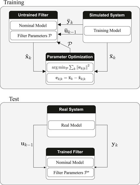
FIGURE 1. Filter parameter optimization. Training: The training is based on a specific system description called training model which is assumed to be the true unknown system model. The training model equals the known nominal system description but with varied system parameters to account for the model uncertainty. The filter runs with the nominal model and its tuning parameters are optimized by comparing the filter estimates with the true states of the training model. Test: The filter is applied to the real system, it runs with the optimized tuning parameters and uses the nominal system description.

5. Stability Analysis of the Adaptive Kalman Filter

As mentioned previously boundedness of the estimation error of SVSF approach (Eqs 3–7) using smoothing boundary layer has never been proven. However, if the adaptive Kalman filter is used instead (${\tilde{\mathbf{M}}}_{k+1}$ is replaced by ${\widehat{\mathbf{K}}}_{k+1}^{\text{opt}}$) the boundedness of the estimation error can be proven as follows.

Theorem 2. The estimation error of the a posteriori estimation

${\widehat{\mathbf{x}}}_{k+1|k+1}={\mathbf{y}}_{k+1}-{\widehat{\mathbf{K}}}_{k+1}^{opt}{\mathbf{e}}_{y_{k+1|k}},(49)$

of the adaptive Kalman filtering approach (Eqs 39–46) is bounded by

$\left|\left|{\mathbf{e}}_{x_{k+1|k+1}}\right|\right|\le \sqrt{\frac{a_2^2}{4{\mathit{ϵ}}_1{\mathit{ϵ}}_2}}\mathbf{R}+a_1,(50)$

if the measurement noise is bounded by $\parallel {\mathbf{r}}_k\parallel <a_1$ and the following conditions are fulfilled

${\mathbf{\Omega }}_k={\widehat{\mathbf{P}}}_{k+1|k}-{\mathit{ϵ}}_1{\mathbf{e}}_{y_{k+1|k}}{\mathbf{e}}_{y_{k+1|k}}^T\ge 0,(51)$

${\mathit{\epsilon }}_1{\mathbf{e}}_{y_{k+1|k}}^T{\left(\mathbf{R}+{\mathbf{\Omega }}_k\right)}^{-1}{\mathbf{e}}_{y_{k+1|k}}\ne 1,(52)$

${\lambda }_{min}\left\{{\left(\mathbf{R}+{\mathbf{\Omega }}_k\right)}^{-1}\right\}>{\mathit{\epsilon }}_2,(53)$

$a_2>\parallel {\left(\mathbf{R}+{\mathbf{\Omega }}_k\right)}^{-1}\parallel ,(54)$

where ${\mathit{\epsilon }}_1$, ${\mathit{\epsilon }}_2$ are sufficient small positive constants, $a_1$, $a_2$ are sufficient large positive constants.

Proof. From Eq. 51 it can be concluded that ${\widehat{\mathbf{P}}}_{k+1|k}$ can be written as

${\widehat{\mathbf{P}}}_{k+1|k}={\mathit{\epsilon }}_1{\mathbf{e}}_{y_{k+1|k}}{\mathbf{e}}_{y_{k+1|k}}^T+{\mathbf{\Omega }}_k,(55)$

with ${\mathbf{\Omega }}_k\mathrm{\succcurlyeq }0$. As known from Eq. 13 the a posteriori estimation error is

${\mathbf{e}}_{x_{k+1|k+1}}={\widehat{\mathbf{K}}}_{k+1}^{\text{opt}}{\mathbf{e}}_{y_{k+1|k}}-{\mathbf{r}}_{k+1}.(56)$

With the definition ${\tilde{\mathbf{R}}}_k=\mathbf{R}+{\mathbf{\Omega }}_k\succ 0$ the estimated optimal filter gain can be written as

${\widehat{\mathbf{K}}}_{k+1}^{\text{opt}}{\mathbf{e}}_{y_{k+1|k}}=\mathbf{R}{\left({\tilde{\mathbf{R}}}_k+{\mathit{ϵ}}_1{\mathbf{e}}_{y_{k+1|k}}{\mathbf{e}}_{y_{k+1|k}}^T\right)}^{-1}{\mathbf{e}}_{y_{k+1|k}}.(57)$

Applying the Sherman-Morrison-Woodbury formular (Fact 2.16.3 [29]) in combination with assumption (Eq. 52) gives

${\left({\tilde{\mathbf{R}}}_k+{\mathit{ϵ}}_1{\mathbf{e}}_{y_{k+1|k}}{\mathbf{e}}_{y_{k+1|k}}^T\right)}^{-1}{\mathbf{e}}_{y_{k+1|k}}={\tilde{\mathbf{R}}}_k^{-1}{\mathbf{e}}_{y_{k+1|k}}-\frac{{\tilde{\mathbf{R}}}_k^{-1}{\mathit{ϵ}}_1{\mathbf{e}}_{y_{k+1|k}}{\mathbf{e}}_{y_{k+1|k}}^T{\tilde{\mathbf{R}}}_k^{-1}{\mathbf{e}}_{y_{k+1|k}}}{1+{\mathbf{e}}_{y_{k+1|k}}^T{\tilde{\mathbf{R}}}_k^{-1}{\mathit{ϵ}}_1{\mathbf{e}}_{y_{k+1|k}}},$

$=\frac{{\tilde{\mathbf{R}}}_k^{-1}{\mathbf{e}}_{y_{k+1|k}}}{1+{\mathit{ϵ}}_1{\mathbf{e}}_{y_{k+1|k}}^T{\tilde{\mathbf{R}}}_k^{-1}{\mathbf{e}}_{y_{k+1|k}}}.(58)$

Using the submultiplicative Frobenius norm (Proposition 9.3.5 [29]) and Eq. 58, Eq. 57 can be written as

$\parallel {\widehat{\mathbf{K}}}_{k+1}^{\text{opt}}{\mathbf{e}}_{y_{k+1|k}}\parallel \le \frac{\parallel \mathbf{R}\parallel \parallel {\tilde{\mathbf{R}}}_k^{-1}\parallel \parallel {\mathbf{e}}_{y_{k+1|k}}\parallel }{1+{\mathit{ϵ}}_1{\mathbf{e}}_{y_{k+1|k}}^T{\tilde{\mathbf{R}}}_k^{-1}{\mathbf{e}}_{y_{k+1|k}}}.(59)$

Based on the minimum eigenvalue of ${\tilde{\mathbf{R}}}_k^{-1}$ the inequality

${\mathit{ϵ}}_1{\lambda }_{\text{min}}\left\{{\tilde{\mathbf{R}}}_k^{-1}\right\}{\left|\left|{\mathbf{e}}_{y_{k+1|k}}\right|\right|}^2\le {\mathit{ϵ}}_1{\mathbf{e}}_{y_{k+1|k}}^T{\tilde{\mathbf{R}}}_k^{-1}{\mathbf{e}}_{y_{k+1|k}},(60)$

can be established (Lemma 8.4.1 [29]). Using Eq. 60 and assumption Eq. 53 an upper bound of Eq. 59 is obtained as

$\parallel {\widehat{\mathbf{K}}}_{k+1}^{\text{opt}}{\mathbf{e}}_{y_{k+1|k}}\parallel \le \frac{\parallel \mathbf{R}\parallel \parallel {\tilde{\mathbf{R}}}_k^{-1}\parallel \parallel {\mathbf{e}}_{y_{k+1|k}}\parallel }{1+{\mathit{ϵ}}_1{\mathit{ϵ}}_2\parallel {\mathbf{e}}_{y_{k+1|k}}{\parallel }^2}.(61)$

Unfortunately, ${\tilde{\mathbf{R}}}_k^{-1}$ implicitly depends on ${\mathbf{e}}_{y_{k+1|k}}$ so that assumption Eq. 54 has to be taken into consideration leading to

$\parallel {\widehat{\mathbf{K}}}_{k+1}^{\text{opt}}{\mathbf{e}}_{y_{k+1|k}}\parallel \le \frac{a_2\parallel \mathbf{R}\parallel \parallel {\mathbf{e}}_{y_{k+1|k}}\parallel }{1+{\mathit{ϵ}}_1{\mathit{ϵ}}_2{\parallel {\mathbf{e}}_{y_{k+1|k}}\parallel }^2}.(62)$

Based on the derivative of Eq. 62 with respect to $\left|\left|{\mathbf{e}}_{y_{k+1|k}}\right|\right|$ it can be shown that the maximum of the upper bound is achieved for $\left|\left|{\mathbf{e}}_{y_{k+1|k}}\right|\right|=\sqrt{\frac{1}{{\mathit{ϵ}}_1{\mathit{ϵ}}_2}}$ which leads to

$\parallel {\widehat{\mathbf{K}}}_{k+1}^{\text{opt}}{\mathbf{e}}_{y_{k+1|k}}\parallel \le \sqrt{\frac{a_2^2}{4{\mathit{ϵ}}_1{\mathit{ϵ}}_2}}\parallel \mathbf{R}\parallel .(63)$

Then (Eq. 50) is proven by applying the triangle inequality on Eq. 56.

6. Numerical Example

In this section state estimation and control of a chemical plant is considered in order to evaluate the performance of original SVSF and the adaptive Kalman filtering variant. According to Ref. 30, Ref. 31 a species A reacts in a continuous stirred tank reactor. The dynamics of the effluent flow concentration $C_A=x_1$ of species A and the reactor temperature $T=x_2$ can be described by the time-continuous model

$\underset{\dot{x}}{\underbrace{\left[\begin{array}{c}{\dot{x}}_1\\ {\dot{x}}_2\end{array}\right]}}=\underset{f\left(\mathbf{x},u\right)}{\underbrace{\left[\begin{array}{c}\frac{q}{V}\left(C_{Af}-x_1\right)-k_0{x}_1\text{exp}\left(-\frac{E}{R{x}_2}\right)\\ a+\frac{UA}{V\rho C_p}\left(u+T_c^{eq}-x_2\right)\end{array}\right],}}(64)$

$a=\frac{q}{V}\left(T_f-x_2\right)+\frac{-\text{Δ}H{k}_0{x}_1}{\rho C_p}\text{exp}\left(-\frac{E}{R{x}_2}\right),$

with measurements $\mathbf{y}$, and control variable z defined as

$\mathbf{y}=\mathbf{x}+\mathbf{r},z=x_1.(65)$

The parameters of the system are shown in Table 2. The input of the system is the change of the coolant stream temperature $u=\text{Δ}{T}_c$ related to the nominal value $T_c^{eq}$. An input saturation of $\left|u\right|\le 50\text{K}$ is considered. The system is simulated based on Euler method using a sampling time of 0.1 s. The resulting discrete-time measurement model is

${\mathbf{y}}_k={\mathbf{x}}_k+{\mathbf{r}}_k,(66)$

where the zero-mean, white noise ${\mathbf{r}}_k$ is Gaussian with covariance

$\mathbf{R}=\left[\begin{array}{cc}{\sigma }_{C_A}^2& 0\\ 0& {\sigma }_T^2\end{array}\right],{\sigma }_{C_A}^2=0.8\frac{{\text{mol}}^2}{{\text{m}}^6},{\sigma }_T^2=0.5{\text{K}}^2.$

For the initial state values $x_1\left(t_0\right)=0.875\text{mol}/\text{l}$, and $x_2\left(t_0\right)=325\text{K}$ are considered.

TABLE 2

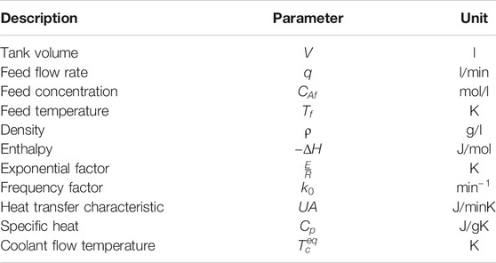
TABLE 2. System parameter description [30].

6.1. Filter Training Process

In the following the optimization of the tuning parameters of A-KF and SVSF approach is considered. As explained in Section 4 variation of the nominal system parameters is required to build the training model. To account for the model uncertainty a variation of 20% of the nominal parameters is considered which is assumed as a priori known. Consequently, the ith parameter of the training model $p_i^{\left(t\right)}$ is obtained from the uniform distribution $p_i^{\left(t\right)}\sim U\left(\left(1+0.2\right)p_i^{\left(0\right)},\left(1-0.2\right)p_i^{\left(0\right)}\right)$. Repeating the step for all parameters $i\in \left\{\mathrm{1,2},\dots ,10\right\}$ forms one training model. The parameter $T_c^{eq}$ is not varied as it is required to be precisely known for control. In Table 3 an overview of the true and nominal system parameters and the parameters used to build the training model is given. In order to account for the different combination and variation of the system parameters three training models are build denoted as Training I, Training II, and Training III.

TABLE 3

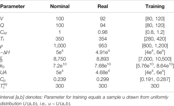
TABLE 3. System parameters of nominal, real, and training model.

For each set the tuning parameters of the filters are optimized separately. The parameters of A-KF approach required to be optimized are given by Eq. 47. For the SVSF approach the boundary layer widths ${\mathbf{\Psi }}_{11}$, ${\mathbf{\Psi }}_{22}$ and convergence rates ${\mathbf{\Phi }}_{11}$, ${\mathbf{\Phi }}_{22}$ of the first and second state are optimized. The optimization is achieved using “genetic algorithm” of MATLAB with default settings. During optimization only one realization of measurement noise is considered so that the costfunction does not vary due to the noise.

The results of optimization are shown in Table 4. The A-KF approach requires at least 60 times more computational time for the optimization than SVSF. The SVSF algorithm is computationally more efficient and in addition it requires less parameters to be optimized. However, the achieved minimal value of the costfunction is always lower in case of A-KF.

TABLE 4

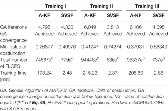
TABLE 4. Computational effort of training process.

6.2. Open Loop Case

In the open loop case the step functions $u=5\text{K}$ and $u=-5\text{K}$ are applied to the system and the resulting step responses are considered for state estimation. The system behavior is simulated over a time horizon of 6 min.

The performance values of A-KF and SVSF approach are shown in Table 5. The filters are applied based on four sets of optimized parameters. Three sets result from Training I, Training II, and Training III. The fourth set denoted as Training I-III considers the mean values of the optimized parameters of the other three sets. As all states are measured the MSE of the measurements is considered also. In order to account for the effect of different noise realizations the results are obtained by simulating the step response 100 times and taking the mean value and variance of the squared estimation error. The filters are applied to the same measurements with same noise realizations. From the results it can be seen that both A-KF and SVSF estimations are more precise than the measurements. In comparison to SVSF the A-KF approach achieves better estimation performance for all considered sets of optimized parameters and both step responses. For one specific run the step responses and the corresponding state estimations are visualized in Figures 2 and 3. The computational time required to generate Table 5 (to simulate both step responses 100 times and apply 8 filters each time) is 18.90 min on a 4xCPU@3.7Ghz with 8 GB memory. The computational time required to apply only one filter on one specific step response is 0.11 s in case of SVSF and 1.49 s in case of A-KF. Both values are far less than the 6 min of simulated system behavior.

TABLE 5

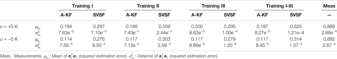
TABLE 5. Estimation performance in open loop case (100 realizations).

FIGURE 2

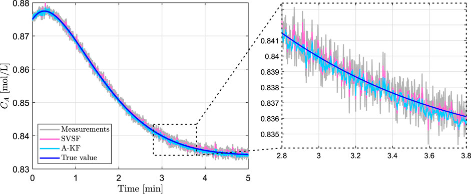
FIGURE 2. Open loop response of step input $u=+5\text{K}$ (Estimation errors of shown realization: ${\mu }_{e_x}^{\text{A}-\text{KF}}=0.193$, ${\mu }_{e_x}^{\text{SVSF}}=0.296$, ${\mu }_{e_x}^{\text{Meas}.}=0.892$).

FIGURE 3

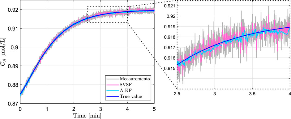
FIGURE 3. Open loop response of step input $u=-5\text{K}$ (Estimation error of shown realization: ${\mu }_{e_x}^{\text{A}-\text{KF}}=0.105$, ${\mu }_{e_x}^{\text{SVSF}}=0.267$, ${\mu }_{e_x}^{\text{Meas}.}=0.886$).

6.3. Closed Loop Case

In the closed loop case the effluent flow concentration $C_A$ of the chemical plant is controlled. The controller relies on the filter estimates. Consequently, the estimation performance as well as the control performance dependent on the filters is studied.

In order to achieve reference tracking of the control variable $C_A$ the super-twisting sliding mode approach [32] is applied. By introducing the estimated tracking error

${\widehat{e}}_r=z_r-\widehat{z},(67)$

with reference value $z_r$ the sliding variable can be calculated as

$\widehat{s}={\dot{\widehat{e}}}_r+\lambda {\widehat{e}}_r,\lambda >0.(68)$

Then reference tracking can be achieved by applying the super-twisting approach [32]

$u=-k_1|\widehat{s}{|}^{\frac{1}{2}}\text{sgn}\left(\widehat{s}\right)-k_2{{\displaystyle \int }}^{\text{}}\text{sgn}\left(\widehat{s}\right)dt(69)$

The controller parameters are chosen as $k_1=0.001$ and $k_2=25$ based on trial and error. For the sliding dynamics $\lambda =0.08$ is considered. The simulated time horizon is 20 min with reference values defined by

$z_r=\{\begin{array}{cc}0.8\text{ mol}/\text{l}& \text{if }t\le 6\text{ min},\\ 0.75\text{ mol}/\text{l}& \text{if }6\text{ min}<t\le 10\text{ min},\\ 0.7\text{ mol}/\text{l}& \text{if }10\text{ min}<t\le 14\text{ min},\\ 0.85\text{ mol}/\text{l}& \text{if }14\text{ min}<t\le 20\text{ min},\end{array}(70)$

where $t\in \left[0\text{ min},20\text{ min}\right]$. Related to the control performance the following four cases are studied. The sliding variable (Eq. 68) is calculated using the estimations of A-KF approach or the estimations of SVSF approach or the measurements denoted as “W/O filters” or the true states denoted as “Optimum”. For the filters the optimized filter parameters of the different training models are considered. The control of the plant over the time horizon of 20 min is simulated 100 times to account for the noise realizations. The measurements used by the filters have same noise realizations. The performance values are shown in Table 6. The best control performance can be achieved based on the true states which are noise-free. Control based on estimations of A-KF or SVSF achieves better performance than applying the controller directly on the noisy measurements. In comparison to SVSF approach A-KF method achieves better reference tracking and more precise state estimation for all considered training models. The control variable and the input values of one specific realization are visualized in Figures 4 and 5. The computational time required to generate Table 6 (to simulate 100 runs of 10 closed loop systems in parallel) is 34.54 min on a 4xCPU@3.7Ghz with 8 GB memory. The computational time required to simulate the closed loop behavior only once based on one controller is 0.45 s if the controller is fed by the estimations of SVSF and 5.24 s if the controller is fed by the estimations of A-KF. This is in both cases far less than the time horizon of 20 min over which the system behavior is simulated.

TABLE 6

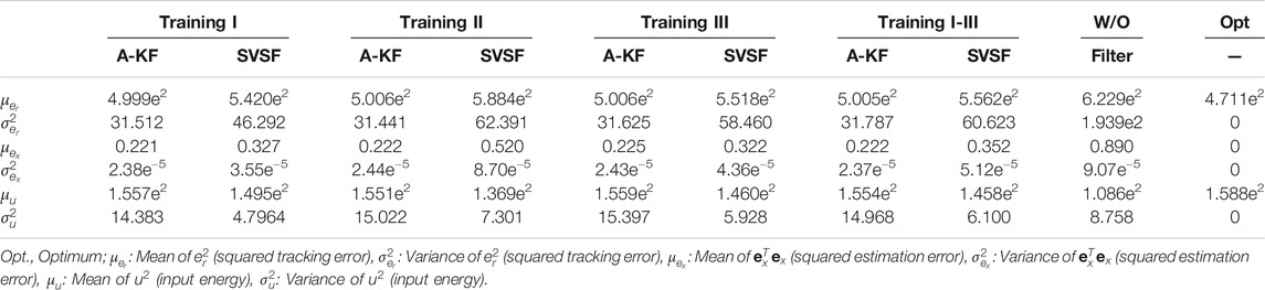
TABLE 6. Control and estimation performance in closed loop case (100 realizations).

FIGURE 4

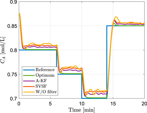
FIGURE 4. Closed loop tracking performance using measured, estimated, or true state values for calculation of the sliding variable (Performance values of shown realization: ${\mu }_{e_r}^{\text{A}-\text{KF}}$ = 5.005e², ${\mu }_{e_r}^{\text{SVSF}}$ = 5.392e², ${\mu }_{e_r}^{\text{W}/\text{O filter}}$ = 6.057e², ${\mu }_{e_r}^{\text{Opt}.}$ = 4.711e²).

FIGURE 5

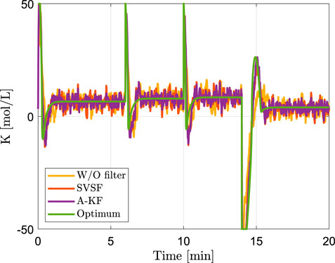
FIGURE 5. Closed loop system inputs generated by controllers (Input energy of shown realization: ${\mu }_u^{\text{A}-\text{KF}}$ = 1.526e², ${\mu }_u^{\text{SVSF}}$ = 1.480e², ${\mu }_u^{\text{W}/\text{O filter}}$ = 1.113e², ${\mu }_u^{\text{Opt}.}$ = 1.588e²).

7. Conclusion

In this paper the relation of smooth variable structure filter (SVSF) and Kalman filter has been studied. An adaptive Kalman filter (A-KF) was derived from the SVSF approach. Sufficient conditions for the boundedness of the estimation error of A-KF approach have been formulated. The simulation results show that beside the SVSF approach also an adaptive Kalman filter can be used to achieve robust estimation performance.

Data Availability Statement

The raw data supporting the conclusions of this article will be made available by the authors, without undue reservation.

Author Contributions

The development and theoretical description of the adaptive Kalman filter approach was undertaken by MS and DS. The numerical simulation was designed and realized by MS. The manuscript was drafted by MS and reviewed by DS.

Conflict of Interest

The authors declare that the research was conducted in the absence of any commercial or financial relationships that could be construed as a potential conflict of interest.

Acknowledgments

The authors want to thank the reviewers for their valueable comments and suggestions.

Footnote

¹The authors thank the anonymous reviewers of European Control Conference 2020 for the insightful comments and suggestions related to the proof of the theorem.

References

1. Kitanidis, PK. Unbiased minimum-variance linear state estimation. Automatica (1987). 23:775–8. doi:10.1016/0005-1098(87)90037-9.

CrossRef Full Text | Google Scholar

2. Gillijns, S, and De Moor, B. Unbiased minimum-variance input and state estimation for linear discrete-time systems. Automatica (2007). 43:111–6. doi:10.1016/j.automatica.2006.08.002.

CrossRef Full Text | Google Scholar

3. Anderson, BD, and Moore, JB. Optimal filtering. Englewood Cliffs, NJ: Prentice-Hall (1979). 256 p.

Google Scholar

4. Hmida, FB, Khémiri, K, Ragot, J, and Gossa, M. Three-stage Kalman filter for state and fault estimation of linear stochastic systems with unknown inputs. J Franklin Inst (2012). 349:2369–88. doi:10.1016/j.jfranklin.2012.05.004.

Google Scholar

5. Dong, Z, and You, Z. Finite-horizon robust Kalman filtering for uncertain discrete time-varying systems with uncertain-covariance white noises. IEEE Signal Process Lett (2006). 13:493–6. doi:10.1109/LSP.2006.873148.

Google Scholar

6. Hassibi, B, Sayed, AH, and Kailath, T. Indefinite quadratic estimation and control: a unified approach to H₂ and H_∞ heories Society for Industrial and Applied Mathematics. Philadelphia, PA (1999). p. 572.

Google Scholar

7. Blom, HAP, and Bar-Shalom, Y. The interacting multiple model algorithm for systems with Markovian switching coefficients. IEEE Trans Automat Contr. (1988). 33:780–3. doi:10.1109/9.1299.

CrossRef Full Text | Google Scholar

8. Martino, L, Read, J, Elvira, V, and Louzada, F. Cooperative parallel particle filters for online model selection and applications to urban mobility. Digit Signal Process (2017). 60:172–85. doi:10.1016/j.dsp.2016.09.011.

CrossRef Full Text | Google Scholar

9. Habibi, S. The smooth variable structure filter. Proc IEEE (2007). 95:1026–59. doi:10.1109/JPROC.2007.893255.

CrossRef Full Text | Google Scholar

10. Gadsden, SA, Song, Y, and Habibi, SR. Novel model-based estimators for the purposes of fault detection and diagnosis. IEEE ASME Trans Mechatron (2013). 18:1237–49. doi:10.1109/TMECH.2013.2253616.

CrossRef Full Text | Google Scholar

11. Kim, T, Wang, Y, Fang, H, Sahinoglu, Z, Wada, T, Hara, S, et al. Model-based condition monitoring for lithium-ion batteries. J Power Sources (2015). 295:16–27. doi:10.1016/j.jpowsour.2015.03.184.

CrossRef Full Text | Google Scholar

12. Qiao, HH, Attari, M, Ahmed, R, Delbari, A, Habibi, S, and Shoa, T. Reliable state of charge and state of health estimation using the smooth variable structure filter. Contr Eng Pract (2018). 77:1–14. doi:10.1016/j.conengprac.2018.04.015.

CrossRef Full Text | Google Scholar

13. Gadsden, SA, Habibi, SR, and Kirubarajan, T. A novel interacting multiple model method for nonlinear target tracking. In: FUSION 2010 : 13th international conference on information fusion; 2010 Jul 26 - 29; Edinburgh, Scotland. Piscataway, NJ: IEEE.

CrossRef Full Text | Google Scholar

14. Attari, M, Gadsden, SA, and Habibi, SR. Target tracking formulation of the SVSF as a probabilistic data association algorithm. In: The 2013 American control conference; 2013 June 17 - 19; Washington, DC; IEEE, Piscataway, NJ. p. 6328–32. doi:10.1109/ACC.2013.6580830.

CrossRef Full Text | Google Scholar

15. Attari, M, Luo, Z, and Habibi, S. An SVSF-based generalized robust strategy for target tracking in clutter. IEEE Trans Intell Transport Syst (2016). 17:1381–92. doi:10.1109/TITS.2015.2504331.

CrossRef Full Text | Google Scholar

16. Luo, Z, Attari, M, Habibi, S, and Mohrenschildt, MV. Online multiple maneuvering vehicle tracking system based on multi-model smooth variable structure filter. IEEE Trans Intell Transport Syst (2020). 21:603–16. doi:10.1109/TITS.2019.2899051.

CrossRef Full Text | Google Scholar

17. Demim, F, Nemra, A, and Louadj, K. Robust SVSF-SLAM for unmanned vehicle in unknown environment. IFAC-PapersOnLine (2016). 49:386–94. doi:10.1016/j.ifacol.2016.10.585.

CrossRef Full Text | Google Scholar

18. Allam, A, Tadjine, M, Nemra, A, and Kobzili, E. Stereo vision as a sensor for SLAM based smooth variable structure filter with an adaptive boundary layer width. In: ICSC 2017, 6th International conference on systems and control. 2017 May 7–9; Batna, Algeria; Piscataway, NJ: IEEE. p. 14–20. doi:10.1109/ICoSC.2017.7958700.

CrossRef Full Text | Google Scholar

19. Liu, Y, and Wang, C. A FastSLAM based on the smooth variable structure filter for UAVs. In: 15th international conference on ubiquitous robots (UR); June 26-30, 2018; Hawaii Convention Center; Piscataway, NJ IEEE (2018). p. 591–6. doi:10.1109/URAI.2018.8441876.

CrossRef Full Text | Google Scholar

20. Ahmed, RM, Sayed, MAE, Gadsden, SA, and Habibi, SR. Fault detection of an engine using a neural network trained by the smooth variable structure filter. In: IEEE international conference on control applications (CCA); Denver, CO; 2011 Sep 28-30; Piscataway, NJ IEEE (2011). p. 1190–6. doi:10.1109/CCA.2011.6044515.

CrossRef Full Text | Google Scholar

21. Al-Shabi, M, and Habibi, S. Iterative smooth variable structure filter for parameter estimation. ISRN Signal Processing (2011). 2011:1. doi:10.5402/2011/725108.

CrossRef Full Text | Google Scholar

22. Spiller, M, Bakhshande, F, and Söffker, D. The uncertainty learning filter: a revised smooth variable structure filter. Signal Process (2018). 152:217–26. doi:10.1016/j.sigpro.2018.05.025.

CrossRef Full Text | Google Scholar

23. Longbin, M, Xiaoquan, S, Yiyu, Z, Kang, SZ, and Bar-Shalom, Y. Unbiased converted measurements for tracking. IEEE Trans Aero Electron Syst (1998). 34:1023–7. doi:10.1109/7.705921.

CrossRef Full Text | Google Scholar

24. Gadsden, SA, and Habibi, SR. A new form of the smooth variable structure filter with a covariance derivation. In: CDC 2010 : 49th IEEE conference on decision and control 2010 Dec 15 - 17; Atlanta, GA; Piscataway, NJ: IEEE (2010). p. 7389–94. doi:10.1109/CDC.2010.5717397.

CrossRef Full Text | Google Scholar

25. Gadsden, SA, El Sayed, M, and Habibi, SR. Derivation of an optimal boundary layer width for the smooth variable structure filter. In: 2011 American Control Conference - ACC 2011; San Francisco, CA; 2011 Jun 29 - Jul 1; Piscataway, NJ: IEEE (2011). p. 4922–7. doi:10.1109/ACC.2011.5990970.

CrossRef Full Text | Google Scholar

26. Tian, Y, Suwoyo, H, Wang, W, and Li, L. An ASVSF-SLAM algorithm with time-varying noise statistics based on MAP creation and weighted exponent. Math Probl Eng. (2019). 2019:1. doi:10.1155/2019/2765731.

CrossRef Full Text | Google Scholar

27. Hide, C, Moore, T, and Smith, M. Adaptive Kalman filtering for low-cost INS/GPS. J Navig. (2003). 56:143–52. doi:10.1017/S0373463302002151.

CrossRef Full Text | Google Scholar

28. Yang, Y, and Gao, W. An optimal adaptive Kalman filter. J Geodes. (2006). 80:177–83. doi:10.1007/s00190-006-0041-0.

CrossRef Full Text | Google Scholar

29. Bernstein, DS. Matrix mathematics: theory, facts, and formulas Princeton, NJ: Princeton University Press (2009). 1184 p.

Google Scholar

30. Magni, L, Nicolao, GD, Magnani, L, and Scattolini, R. A stabilizing model-based predictive control algorithm for nonlinear systems. Automatica (2001). 37:1351–62. doi:10.1016/S0005-1098(01)00083-8.

CrossRef Full Text | Google Scholar

31. Seborg, DE, Mellichamp, DA, Edgar, TF, and Doyle, FJ. Process dynamics and control New York, NY: John Wiley & Sons (2010). p. 1085–6.

Google Scholar

32. Shtessel, Y, Edwards, C, Fridman, L, and Levant, A. Sliding mode control and observation. New York: Springer (2014). 356 p.

Google Scholar