The Mathematical Structure of Integrated Information Theory

1 Introduction

Integrated Information Theory (IIT), developed by Giulio Tononi and collaborators [5, 45–47], has emerged as one of the leading scientific theories of consciousness. At the heart of the latest version of the theory [19, 25, 26, 31, 40] is an algorithm which, based on the level of integration of the internal functional relationships of a physical system in a given state, aims to determine both the quality and quantity (‘$\Phi$ value’) of its conscious experience.

While promising in itself [12, 43], the mathematical formulation of the theory is not satisfying to date. The presentation in terms of examples and accompanying explanation veils the essential mathematical structure of the theory and impedes philosophical and scientific analysis. In addition, the current definition of the theory can only be applied to comparably simple classical physical systems [1], which is problematic if the theory is taken to be a fundamental theory of consciousness, and should eventually be reconciled with our present theories of physics.

To resolve these problems, we examine the essentials of the IIT algorithm and formally define a generalized notion of Integrated Information Theory. This notion captures the inherent mathematical structure of IIT and offers a rigorous mathematical definition of the theory which has ‘classical’ IIT 3.0 of Tononi et al. [25, 26, 31] as well as the more recently introduced Quantum Integrated Information Theory of Zanardi, Tomka and Venuti [50] as special cases. In addition, this generalization allows us to extend classical IIT, freeing it from a number of simplifying assumptions identified in [3]. Our results are summarised in Figure 1.

FIGURE 1

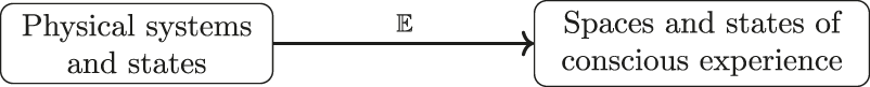
FIGURE 1. An Integrated Information Theory specifies for every system in a particular state its conscious experience, described formally as an element of an experience space. In our formalization, this is a map $\mathbf{Sys}\stackrel{\mathbb{E}}{\to }\mathbf{Exp}$ from the system class Sys into a class Exp of experience spaces, which, first, sends each system S to its space of possible experiences $\mathbb{E}\left(S\right)$, and, second, sends each state $s\in \text{St}\left(S\right)$ to the actual experience the system is having when in that space, $\text{St}\left(S\right)\to \mathbb{E}\left(S\right)s\mapsto \mathbb{E}\left(S,s\right).$ The definition of this map in terms of axiomatic descriptions of physical systems, experience spaces and further structure used in classical IIT is given in the first half of this paper.

In the associated article [44] we show more generally how the main notions of IIT, including causation and integration, can be treated, and an IIT defined, starting from any suitable theory of physical systems and processes described in terms of category theory. Restricting to classical or quantum process then yields each of the above as special cases. This treatment makes IIT applicable to a large class of physical systems and helps overcome the current restrictions.

Our definition of IIT may serve as the starting point for further mathematical analysis of IIT, in particular if related to category theory [30, 49]. It also provides a simplification and mathematical clarification of the IIT algorithm which extends the technical analysis of the theory [1, 41, 42] and may contribute to its ongoing critical discussion [2, 4, 8, 23, 27, 28, 33]. The concise presentation of IIT in this article should also help to make IIT more easily accessible for mathematicians, physicists and other researchers with a strongly formal background.

This work is concerned with the most recent version of IIT as proposed in [25, 26, 31, 40] and similar papers quoted below. Thus our constructions recover the specific theory of consciousness referred to as IIT 3.0 or IIT 3.x, which we will call classical IIT in what follows. Earlier proposals by Tononi et al. that also aim to explicate the general idea of an essential connection between consciousness and integrated information constitute alternative theories of consciousness which we do not study here. A yet different approach would be to take the term ‘Integrated Information Theory’ to refer to the general idea of associating conscious experience with some pre-theoretic notion of integrated information, and to explore the different ways that this notion could be defined in formal terms [4, 27, 28, 37].

Relation to Other Work

This work develops a thorough mathematical perspective of one of the promising contemporary theories of consciousness. As such it is part of a number of recent contributions which seek to explore the role and prospects of mathematical theories of consciousness [11, 15, 18, 30, 49], to help overcome problems of existing models [17, 18, 34] and to eventually develop new proposals [6, 13, 16, 20, 22, 29, 39].

1.1 Structure of Article

We begin by introducing the necessary ingredients of a generalised Integrated Information Theory in Sections 2–4, namely physical systems, experience spaces and cause-effect repertoires. Our approach is axiomatic in that we state only the precise formal structure which is necessary to apply the IIT algorithm. We neither motivate nor criticize these structures as necessary or suitable to model consciousness. Our goal is simply to recover IIT 3.0. In Section 5, we introduce a simple formal tool which allows us to present the definition of the algorithm of an IIT in a concise form in Sections 6 and 7. Finally, in Section 8, we summarise the full definition of such a theory. The result is the definition of a generalized IIT. We call any application of this definition ‘an IIT’.

Following this we give several examples including IIT 3.0 in Section 9 and Quantum IIT in Section 10. In Section 11 we discuss how our formulation allows one to extend classical IIT in several fundamental ways, before discussing further modifications to our approach and other future work in Section 12. Finally, the appendix includes a detailed explanation of how our generalization of IIT coincides with its usual presentation in the case of classical IIT.

2 Systems

The first step in defining an Integrated Information Theory (IIT) is to specify a class $\mathbf{Sys}$ of physical systems to be studied. Each element $S\in \mathbf{Sys}$ is interpreted as a model of one particular physical system. In order to apply the IIT algorithm, it is only necessary that each element S come with the following features.

Definition 1. A system class$\mathbf{Sys}$ is a class each of whose elements S, called systems, come with the following data:

1. A set $\text{St}\left(S\right)$ of states;

2. for every $s\in \text{St}\left(S\right)$, a set ${\text{Sub}}_s\left(S\right)\subset \mathbf{S}\mathbf{y}\mathbf{s}$ of subsystems and for each $M\in {\text{Sub}}_s\left(S\right)$ an induced state $s{|}_M\in \text{St}\left(M\right)$;

3. a set ${\mathbb{D}}_S$ of decompositions, with a given trivial decomposition$1\in {\mathbb{D}}_S$;

4. for each $z\in {\mathbb{D}}_S$ a corresponding cut system$S^z\in \mathbf{S}\mathbf{y}\mathbf{s}$ and for each state $s\in \text{St}\left(S\right)$ a corresponding cut state$s^z\in \text{St}\left(S^z\right)$.

Moreover, we require that $\mathbf{S}\mathbf{y}\mathbf{s}$ contains a distinguished empty system, denoted I, and that $I\in \text{Sub}\left(S\right)$ for all S. For the IIT algorithm to work, we need to assume furthermore that the number of subsystems remains the same under cuts or changes of states, i.e. that we have bijections ${\text{Sub}}_s\left(S\right)\simeq {\text{Sub}}_{s\text{'}}\left(S\right)$ for all $s,s\text{'}\in \text{St}\left(S\right)$ and ${\text{Sub}}_s\left(S\right)\simeq {\text{Sub}}_{s^z}\left(S^z\right)$ for all $z\in {\mathbb{D}}_S.$Note that taking a subsystem of a system S requires specifying a state s of S. An example class of systems is illustrated in Figure 2. In this article we will assume that each set ${\text{Sub}}_s\left(S\right)$ is finite, discussing the extension to the infinite case in Section 12. We will give examples of system classes and for all following definitions in Sections 9 and 10.

FIGURE 2

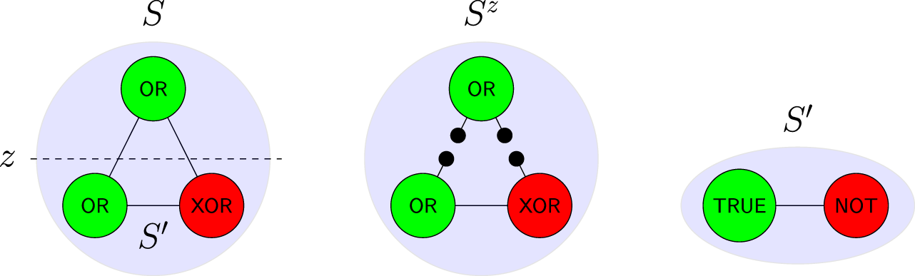
FIGURE 2. As an example of Definition 1 similar to IIT 3.0, consider simple systems given by sets of nodes (or ‘elements’), with a state assigning each node the state ‘on’ (depicted green) or ‘off’ (red). Each system comes with a time evolution shown by labelling each node with how its state in the next time-step depends on the states of the others. Decompositions of a system S correspond to binary partition of the nodes, such as z above. The cut system $S^{\mathit{z}}$ is given by modifying the time evolution of S so that the two halves do not interact; in this case all connections between the halves are replaced by sources of noise which send ‘on’ or ‘off’ with equal likelihood, depicted as black dots above. Given a current state s of S, any subset of the nodes (such as those below the dotted line) determines a subsystem ${\mathit{S}}^{\prime }$, with time evolution obtained from that of S by fixing the nodes in $\mathit{S}\mathrm{\setminus }{\mathit{S}}^{\prime }$ (here, the upper node) to be in the state specified by s. Note that while in this example any subsystem (subset of S) determines a decomposition (partition of S) we do not require such a relationship in general.

3 Experience

An IIT aims to specify for each system in a particular state its conscious experience. As such, it will require a mathematical model of such experiences. Examining classical IIT, we find the following basic features of the final experiential states it describes which are needed for its algorithm.

Firstly, each experience e should crucially come with an intensity, given by a number $\left|\right|e\left|\right|$ in the non-negative reals ${\mathrm{ℝ}}^{+}$ (including zero). This intensity will finally correspond to the overall intensity of experience, usually denoted by $\text{Φ}$. Next, in order to compare experiences, we require a notion of distance d(e,e′) between any pair of experiences e,e′. Finally, the algorithm will require us to be able to rescale any given experience e to have any given intensity. Mathematically, this is most easily encoded by letting us multiply any experience e by any number $r\in {\mathrm{ℝ}}^{+}$. In summary, a minimal model of experience in a generalized IIT is the following.

Definition 2. An experience space is a set E with:

1. An intensity function $\left|\right|.\left|\right|:E\to {\mathrm{ℝ}}^{+}$

2. A distance function $d:E\times E\to {\mathrm{ℝ}}^{+}$

3. A scalar multiplication${\mathrm{ℝ}}^{+}\times E\to E$, denoted $\left(r,e\right)\mapsto r\cdot e$, satisfying

$\Vert r\cdot e\Vert =r\cdot \Vert e\Vert r\cdot \left(s\cdot e\right)=\left(rs\right)\cdot e1\cdot e=e$

for all $e\in E$ and $r,s\in {\mathrm{ℝ}}^{+}$.

We remark that this same axiomatisation will apply both to the full space of experiences of a system, as well as to the spaces describing components of the experiences (‘concepts’ and ‘proto-experiences’ defined in later sections). We note that the distance function does not necessarily have to satisfy the axioms of a metric. While this and further natural axioms such as $d\left(r\cdot e,r\cdot f\right)=r\cdot d\left(e,f\right)$ might hold, they are not necessary for the IIT algorithm.The above definition is very general, and in any specific application of IIT, the experiences may come with further mathematical structure. The following example includes the experience spaces used in classical IIT.

Example 3. Any metric space $\left(X,d\right)$ may be extended to an experience space $\overline{X}:=X\times {\mathrm{ℝ}}^{+}$ in various ways. E.g., one can define $\left|\right|\left(x,r\right)\left|\right|=r$, $r\cdot \left(x,s\right)=\left(x,rs\right)$ and define the distance as

$d\left(\left(x,r\right),\left(y,s\right)\right)=rd\left(x,y\right)(1)$

This is the definition used in classical IIT (cf. Section 9 and Appendix A). An important operation on experience spaces is taking their product.

Definition 4. For experience spaces E and F, we define the product to be the space $E\times F$ with distance

$d\left(\left(e,f\right),\left(e^{\prime },f^{\prime }\right)\right)=d\left(e,e^{\prime }\right)+d\left(f,f^{\prime }\right),(2)$

intensity $\Vert \left(e,f\right)\Vert =\max \left\{\Vert e\Vert ,\Vert f\Vert \right\}$ and scalar multiplication $r\cdot \left(e,f\right)=\left(r\cdot e,r\cdot f\right)$. This generalizes to any finite product ${\displaystyle \prod }_{i\in I}{E}_i$ of experience spaces.

4 Repertoires

In order to define the experience space and individual experiences of a system S, an IIT utilizes basic building blocks called ‘repertoires’, which we will now define. Next to the specification of a system class, this is the essential data necessary for the IIT algorithm to be applied.

Each repertoire describes a way of ‘decomposing’ experiences, in the following sense. Let D denote any set with a distinguished element 1, for example the set ${\mathbb{D}}_S$ of decompositions of a system S, where the distinguished element is the trivial decomposition $1\in {\mathbb{D}}_S$.

Definition 5. Let e be an element of an experience space E. A decomposition of e over D is a mapping $\overline{e}:D\to E$ with $\overline{e}\left(1\right)=e$.In more detail, a repertoire specifies a proto-experience for every pair of subsystems and describes how this experience changes if the subsystems are decomposed. This allows one to assess how integrated the system is with respect to a particular repertoire. Two repertoires are necessary for the IIT algorithm to be applied, together called the cause-effect repertoire.For subsystems $M,P\in {\text{Sub}}_s\left(S\right)$, define ${\mathbb{D}}_{M,P}:={\mathbb{D}}_M\times {\mathbb{D}}_P$. This set describes the decomposition of both subsystems simultaneously. It has a distinguished element $1=\left(1_M,1_P\right)$.

Definition 6. A cause-effect repertoire at S is given by a choice of experience space $\mathrm{\mathbb{P}}\mathbb{E}\left(S\right)$, called the space of proto-experiences, and for each $s\in \text{St}\left(S\right)$ and $M,P\in {\text{Sub}}_s\left(S\right)$, a pair of elements

$\mathrm{cau}{\mathrm{s}}_s\left(M,P\right),\mathrm{ef}{\mathrm{f}}_s\left(M,P\right)\in \mathrm{\mathbb{P}}\mathbb{E}\left(S\right)(3)$

and for each of them a decomposition over ${\mathbb{D}}_{M,P}$.Examples of cause-effect repertoires will be given in Sections 9 and 10. A general definition in terms of process theories is given in [44]. For the IIT algorithm, a cause-effect repertoire needs to be specified for every system S, as in the following definition.

Definition 7. A cause-effect structure is a specification of a cause-effect repertoire for every $S\in \mathbf{S}\mathbf{y}\mathbf{s}$ such that

$\mathrm{\mathbb{P}}\mathbb{E}\left(S\right)=\mathrm{\mathbb{P}}\mathbb{E}\left(S^z\right) \text{for all} z\in {\mathbb{D}}_S.(4)$

The names ‘cause’ and ‘effect’ highlight that the definitions of ${\text{caus}}_s\left(M,P\right)$ and ${\text{eff}}_s\left(M,P\right)$ in classical and Quantum IIT describe the causal dynamics of the system. They are intended to capture the manner in which the ‘current’ state s of the system, when restricted to M, constrains the ‘previous’ or ‘next’ state of P, respectively.

5 Integration

We have now introduced all of the data required to define an IIT; namely, a system class along with a cause-effect structure. From this, we will give an algorithm aiming to specify the conscious experience of a system. Before proceeding to do so, we introduce a conceptual short-cut which allows the algorithm to be stated in a concise form. This captures the core ingredient of an IIT, namely the computation of how integrated an entity is.

Definition 8. Let E be an experience space and e an element with a decomposition over some set D. The integration level of e relative to this decomposition is

$\varphi \left(e\right):=\underset{1\ne z\in D}{\min }d\left(e,\overline{e}\left(z\right)\right).(5)$

Here, d denotes the distance function of E, and the minimum is taken over all elements of D besides 1. The integration scaling of e is then the element of E defined by

$\iota \left(e\right):=\varphi \left(e\right)\cdot \widehat{e},(6)$

where $\widehat{e}$ denotes the normalization of e, defined as

$\widehat{e}:=\{\begin{array}{cc}\frac{1}{\Vert e\Vert }\cdot e& \text{ if }\Vert e\Vert \ne 0\\ e& \text{ if }\Vert e\Vert =0.\end{array}$

Finally, the integration scaling of a pair $e_1,e_2$ of such elements is the pair

$\iota \left(e_1,e_2\right):=\left(\varphi \cdot \widehat{e_1},\varphi \cdot \widehat{e_2}\right)(7)$

where $\varphi :=\text{min}\left(\varphi \left(e_1\right),\varphi \left(e_2\right)\right)$ is the minimum of their integration levels.We will also need to consider indexed collections of decomposable elements. Let S be a system in a state $s\in \text{St}\left(S\right)$ and assume that for every $M\in {\text{Sub}}_s\left(S\right)$ an element $e_M$ of some experience space $E_M$ with a decomposition over some $D_M$ is given. We call ${\left(e_M\right)}_{M\in {\text{Sub}}_s\left(S\right)}$ a collection of decomposable elements, and denote it as ${\left(e_M\right)}_M$.

Definition 9. The core of the collection ${\left(e_M\right)}_M$ is the subsystem $C\in {\text{Sub}}_s\left(S\right)$ for which $\varphi \left(e_C\right)$ is maximal.¹ The core integration scaling of the collection is $\iota \left(e_C\right)$. The core integration scaling of a pair of collections $\left({\left(e_M\right)}_M,{\left(f_M\right)}_M\right)$ is $\iota \left(e_C,f_D\right)$, where $C,D$ are the cores of ${\left(e_M\right)}_M$ and ${\left(f_M\right)}_M$, respectively.

6 Constructions: Mechanism Level

Let $S\in \mathbf{S}\mathbf{y}\mathbf{s}$ be a physical system whose experience in a state $s\in \text{St}\left(S\right)$ is to be determined. The first level of the algorithm involves fixing some subsystem $M\in {\text{Sub}}_s\left(S\right)$, referred to as a ‘mechanism’, and associating to it an object called its ‘concept’ which belongs to the concept space

$\mathrm{ℂ}\left(S\right):=\mathrm{\mathbb{P}}\mathbb{E}\left(S\right)\times \mathrm{\mathbb{P}}\mathbb{E}\left(S\right).(8)$

For every choice of $P\in {\text{Sub}}_s\left(S\right)$, called a ‘purview’, the repertoire values ${\text{caus}}_s\left(M,P\right)$ and ${\text{eff}}_s\left(M,P\right)$ are elements of $\mathrm{\mathbb{P}}\mathbb{E}\left(S\right)$ with given decompositions over ${\mathbb{D}}_{M,P}$. Fixing M, they provide elements with decompositions over Sub(S) given by

$\begin{array}{c}{\text{caus}}_s\left(M\right):={\left({\text{caus}}_s\left(M,P\right)\right)}_{P\in \text{Sub}\left(S\right)}\\ {\text{eff}}_s\left(M\right):={\left({\text{eff}}_s\left(M,P\right)\right)}_{P\in \text{Sub}\left(S\right)}.\end{array}(9)$

The concept of M is then defined as the core integration scaling of this pair of collections,

${ℂ}_{S,s}\left(M\right):=\text{Core integration scaling of} \left({\text{caus}}_s\left(M\right),{\text{eff}}_s\left(M\right)\right).(10)$

It is an element of $\mathrm{ℂ}\left(S\right)$. Unraveling our definitions, the concept thus consists of the values of the cause and effect repertoires at their respective ‘core’ purviews $P^c,P^e$, i.e. those which make them ‘most integrated’. These values $\text{caus}\left(M,P^c\right)$ and $\text{eff}\left(M,P^e\right)$ are then each rescaled to have intensity given by the minima of their two integration levels.

7 Constructions: System Level

The second level of the algorithm specifies the experience of system S in state s. To this end, all concepts of a system are collected to form its Q-shape, defined as

${\mathrm{\mathbb{Q}}}_s\left(S\right):={\left({\mathrm{ℂ}}_{S,s}\left(M\right)\right)}_{M\in {\text{Sub}}_s\left(S\right)}.(11)$

This Is an Element of the Space

$\mathbb{E}\left(S\right)=\mathrm{ℂ}{\left(S\right)}^{n\left(S\right)},(12)$

where $n\left(S\right):=\left|{\text{Sub}}_s\left(S\right)\right|$, which is finite and independent of the state s according to our assumptions. We can also define a Q-shape for any cut of S. Let $z\in {\mathbb{D}}_S$ be a decomposition, $S^z$ the corresponding cut system and $s^z$ be the corresponding cut state. We define

${\mathrm{\mathbb{Q}}}_s\left(S^z\right):={\left({\mathrm{ℂ}}_{S^z,s^z}\left(M\right)\right)}_{M\in {\text{Sub}}_{s^z}\left(S^z\right)}.(13)$

Because of Eq. 4, and since the number of subsystems remains the same when cutting, ${\mathrm{\mathbb{Q}}}_s\left(S^z\right)$ is also an element of $\mathbb{E}\left(S\right)$. This gives a map

$\begin{array}{c}{\overline{\mathbb{Q}}}_{S,s}:{\mathbb{D}}_S\to \mathbb{E}\left(S\right)\\ z\mapsto {\mathbb{Q}}_s\left(S^z\right)\end{array}$

which is a decomposition of ${\mathrm{\mathbb{Q}}}_s\left(S\right)$ over ${\mathbb{D}}_S$. Considering this map for every subsystem of S gives a collection of decompositions defined as

$\mathrm{\mathbb{Q}}\left(S,s\right):={\left({\overline{\mathrm{\mathbb{Q}}}}_{M,s{|}_M}\right)}_{M\in {\text{Sub}}_s\left(S\right)}$

This is the system level-object of relevance and is what specifies the experience of a system according to IIT.

Definition 10. The experience of system S in the state $s\in \text{St}\left(S\right)$ is

$\mathbb{E}\left(S,s\right):=\text{Core integration scaling of }\mathrm{\mathbb{Q}}\left(S,s\right).(14)$

The definition implies that $\mathbb{E}\left(S,s\right)\in \mathbb{E}\left(M\right)$, where $M\in {\text{Sub}}_s\left(S\right)$ is the core of the collection $\mathrm{\mathbb{Q}}\left(S,s\right)$, called the major complex. It describes which part of system S is actually conscious. In most cases there will be a natural embedding $\mathbb{E}\left(M\right)\to \mathbb{E}\left(S\right)$ for a subsystem M of S, allowing us to view $\mathbb{E}\left(S,s\right)$ as an element of $\mathbb{E}\left(S\right)$ itself. Assuming this embedding to exist allows us to define an Integrated Information Theory concisely in the next section.

8 Integrated Information Theories

We can now summarize all that we have said about IITs.

Definition 11. An Integrated Information Theory is determined as follows. The data of the theory is a system class $\mathbf{S}\mathbf{y}\mathbf{s}$ along with a cause-effect structure. The theory then gives a mapping

$\mathbf{Sys}\stackrel{\mathbb{E}}{\to }\mathbf{Exp}(15)$

into the class $\mathbf{E}\mathbf{x}\mathbf{p}$ of all experience spaces, sending each system S to its space of experiences $\mathbb{E}\left(S\right)$ defined in Eq. 12, and a mapping

$\begin{array}{cc}\mathrm{St}\left(S\right)& \to \mathbb{E}\left(S\right)\\ s& \mapsto \mathbb{E}\left(S,s\right)\end{array}(16)$

which determines the experience of the system when in a state s, defined in Eq. 14.The quantity of the system’s experience is given by

$\Phi \left(S,s\right):=\Vert \mathbb{E}\left(S,s\right)\Vert ,$

and the quality of the system’s experience is given by the normalized experience $\widehat{\mathbb{E}}\left(S,s\right)$. The experience is “located” in the core of the collection $\mathrm{\mathbb{Q}}\left(S,s\right)$, called the major complex, which is a subsystem of S.In the next sections we specify the data of several example IITs.

9 Classical IIT

In this section we show how IIT 3.0 [25, 26, 31, 48] fits in into the framework developed here. A detailed explanation of how our earlier algorithm fits with the usual presentation of IIT is given in Appendix A. In [44] we give an alternative categorical presentation of the theory.

9.1 Systems

We first describe the system class underlying classical IIT. Physical systems S are considered to be built up of several components $S_1,\dots ,S_n$, called elements. Each element $S_i$ comes with a finite set of states $\text{St}\left(S_i\right)$, equipped with a metric. A state of S is given by specifying a state of each element, so that

$\text{St}\left(S\right)=\text{St}\left(S_1\right)\times \cdots \times \text{St}\left(S_n\right).(17)$

We define a metric d on $\text{St}\left(S\right)$ by summing over the metrics of the element state spaces $\text{St}\left(S_i\right)$ and denote the collection of probability distributions over $\text{St}\left(S\right)$ by $\mathcal{P}\left(S\right)$. Note that we may view $\text{St}\left(S\right)$ as a subset of $\mathcal{P}\left(S\right)$ by identifying any $s\in \text{St}\left(S\right)$ with its Dirac distribution ${\delta }_s\in \mathcal{P}\left(S\right)$, which is why we abbreviate ${\delta }_s$ by s occasionally in what follows.

Additionally, each system comes with a probabilistic (discrete) time evolution operator or transition probability matrix, sending each $s\in \text{St}\left(S\right)$ to a probabilistic state $T\left(s\right)\in \mathcal{P}\left(S\right)$. Equivalently it may be described as a convex-linear map

$T:\mathcal{P}\left(S\right)\to \mathcal{P}\left(S\right).(18)$

Furthermore, the evolution T is required to satisfy a property called conditional independence, which we define shortly.

The class $\mathbf{S}\mathbf{y}\mathbf{s}$ consists of all possible tuples $S=\left({\left\{S_i\right\}}_{i=1}^n,T\right)$ of this kind, with the trivial system I having only a single element with a single state and trivial time evolution.

9.2 Conditioning and Marginalizing

In what follows, we will need to consider two operations on the map T. Let M be any subset of the elements of a system and $M^{\perp }$ its complement. We again denote by $\text{St}\left(M\right)$ the Cartesian product of the states of all elements in M, and by $\mathcal{P}\left(M\right)$ the probability distributions on $\text{St}\left(M\right)$. For any $p\in \mathcal{P}\left(M\right)$, we define the conditioning [26] of T on p as the map

$\begin{array}{c}T|p\rangle :\mathcal{P}\left(M^{\perp }\right)\to \mathcal{P}\left(S\right)\\ p^{\prime }\mapsto T\left(p\cdot p^{\prime }\right)\end{array}(19)$

where $p\cdot p^{\prime }$ denotes the multiplication of these probability distributions to give a probability distribution over S. Next, we define marginalisation over M as the map

$\langle M|:\mathcal{P}\left(S\right)\to \mathcal{P}\left(M^{\perp }\right)(20)$

such that for each $p\in \mathcal{P}\left(S\right)$ and $m_2\in \text{St}\left(M^{\perp }\right)$ we have

$\langle M|p\left(m_2\right)={\displaystyle \sum }_{m_1\in \text{St}\left(M\right)}p\left(m_1,m_2\right).(21)$

In particular for any map T as above we call $\langle M|T$ the marginal of T over M and we write $T_i:=\langle S_i^{\perp }|T$ for each $i=1,\dots ,n$. Conditional independence of T may now be defined as the requirement that

$T\left(p\right)=\underset{i=1}{{\displaystyle \prod }^n}{T}_i\left(p\right) \text{for all} p\in \mathcal{P}\left(S\right),$

where the right-hand side is again a probability distribution over $\text{St}\left(S\right)$.

9.3 Subsystems, Decompositions and Cuts

Let a system S in a state $s\in \text{St}\left(S\right)$ be given. The subsystems are characterized by subsets of the elements that constitute S. For any subset $M=\left\{S_1,\dots ,S_m\right\}$ of the elements of S, the corresponding subsystem is also denoted M and $\text{St}\left(M\right)$ is again given by the product of the $\text{St}\left(S_i\right)$, with time evolution

$T_M:=\langle M^{\perp }\left|T\right|s_{M^{\perp }}\rangle ,(22)$

where $s_{M^{\perp }}$ is the restriction of the state s to $\text{St}\left(M^{\perp }\right)$ and $|s_{M^{\perp }}\rangle$ denotes the conditioning on the Dirac distribution ${\delta }_{s_{M^{\perp }}}$.

The decomposition set ${\mathbb{D}}_S$ of a system S consists of all partitions of the set N of elements of S into two disjoint sets M and $M^{\perp }$. We denote such a partition by $z=\left(M,M^{\perp }\right)$. The trivial decomposition 1 is the pair $\left(N,\varnothing \right)$.

For any decomposition $\left(M,M^{\perp }\right)$ the corresponding cut system $S^{\left(M,M^{\perp }\right)}$ is the same as S but with a new time evolution $T^{\left(M,M^{\perp }\right)}$. Using conditional independence, it may be defined for each $i=1,\dots ,n$ as

$T_i^{\left(M,M^{\perp }\right)}:=\{\begin{array}{cc}{T}_i& i\in M^{\perp }\\ T_i|{\omega }_{M^{\perp }}\rangle \langle M^{\perp }|& i\in M\end{array},(23)$

where ${\omega }_M\in \mathcal{P}\left(M\right)$ denotes the uniform distribution on $\text{St}\left(M\right)$. This is interpreted in the graph depiction as removing all those edges from the graph whose source is in $M^{\perp }$ and whose target is in M. The corresponding input of the target element is replaced by noise, i.e. the uniform probability distribution over the source element.

9.4 Proto-Experiences

For each system S, the first Wasserstein metric (or ‘Earth Mover’s Distance’) makes $\mathcal{P}\left(S\right)$ a metric space $\left(\mathcal{P}\left(S\right),d\right)$. The space of proto-experiences of classical IIT is

$\mathrm{\mathbb{P}}\mathbb{E}\left(S\right):=\overline{\mathcal{P}\left(S\right)},(24)$

where $\overline{\mathcal{P}\left(S\right)}$ is defined in Example 3. Thus elements of $\mathrm{\mathbb{P}}\mathbb{E}\left(S\right)$ are of the form $\left(p,r\right)$ for some $p\in \mathcal{P}\left(S\right)$ and $r\in {\mathrm{ℝ}}^{+}$, with distance function, intensity and scalar multiplication as defined in the example.

9.5 Repertoires

It remains to define the cause-effect repertoires. Fixing a state s of S, the first step will be to define maps ${\text{caus}}_{\text{s}}^{\prime }$ and ${\text{eff}}_s^{\prime }$ which send any choice of $\left(M,P\right)\in \text{Sub}\left(S\right)\times \text{Sub}\left(S\right)$ to an element of $\mathcal{P}\left(P\right)$. These should describe the way in which the current state of M constrains that of P in the next or previous time-steps. We begin with the effect repertoire. For a single element purview $P_i$ we define

${\text{eff}}_s^{\prime }\left(M,P_i\right):=\langle P_i^{\perp }|T|{\omega }_{M^{\perp }}\rangle \left(s_M\right),(25)$

where $s_M$ denotes (the Dirac distribution of) the restriction of the state s to M. While it is natural to use the same definition for arbitrary purviews, IIT 3.0 in fact uses another definition based on consideration of ‘virtual elements’ [25, 26, 48], which also makes calculations more efficient (Supplementary Material S1 of [26]). For general purviews P, this definition is

${\text{eff}}_s^{\prime }\left(M,P\right)={\displaystyle \prod }_{P_i\in P}{\text{eff}}_s^{\prime }\left(M,P_i\right),(26)$

taking the product over all elements $P_i$ in the purview P. Next, for the cause repertoire, for a single element mechanism $M_i$ and each $\tilde{s}\in \text{St}\left(P\right)$, we define

${\text{caus}}_s^{\prime }\left(M_i,P\right)\left[\tilde{s}\right]=\lambda \langle M_i^{\perp }|T|{\omega }_{P^{\perp }}\rangle \left({\delta }_{\tilde{s}}\right)\left[s_{M_i}\right],(27)$

where λ is the unique normalisation scalar making ${\text{caus}}_s^{\prime }\left(M_i,P\right)$ a valid element of $\mathcal{P}\left(P\right)$. Here, for clarity, we have indicated evaluation of probability distributions at particular states by square brackets. If the time evolution operator has an inverse $T^{-1}$, this cause repertoire could be defined similarly to (25) by ${\text{caus}}_{\text{s}}^{\prime }\left(M_i,P\right)=\langle P^{\perp }\left|T^{-1}\right|{\omega }_{M_i^{\perp }}\rangle \left(s_{M_i}\right),$ but classical IIT does not utilize this definition.

For General Mechanisms M, we Then Define

${\text{caus}}_{\text{s}}^{\prime }\left(M,P\right)=\kappa {\displaystyle \prod }_{M_i\in M}{\text{caus}}_{\text{s}}^{\prime }\left(M_i,P\right)(28)$

where the product is over all elements $M_i$ in M and where $\kappa \in {\mathrm{ℝ}}^{+}$ is again a normalisation constant. We may at last now define

$\begin{array}{cc}{\text{caus}}_s\left(M,P\right)& :={\text{caus}}_{\text{s}}^{\prime }\left(M,P\right)\cdot {\text{caus}}_{\text{s}}^{\prime }\left(\varnothing ,P^{\perp }\right)\\ {\text{eff}}_s\left(M,P\right)& :={\text{eff}}_{\text{s}}^{\prime }\left(M,P\right)\cdot {\text{eff}}_{\text{s}}^{\prime }\left(\varnothing ,P^{\perp }\right),\end{array}(29)$

with intensity 1 when viewed as elements of $\mathrm{\mathbb{P}}\mathbb{E}\left(S\right)$. Here, the dot indicates again the multiplication of probability distributions and $\varnothing$ denotes the empty mechanism.

The distributions ${\text{caus}}_{\text{s}}^{\prime }\left(\varnothing ,P^{\perp }\right)$ and ${\text{eff}}_s^{\prime }\left(\varnothing ,P^{\perp }\right)$ are called the unconstrained cause and effect repertoires over $P^{\perp }$.

Remark 12. It is in fact possible for the right-hand side of Eq. 28 to be equal to 0 for all $\tilde{s}$ for some $M_i\in M$. In this case we set ${\text{caus}}_{\text{s}}^{\prime }\left(M,P\right)=\left({\omega }_S,0\right)$ in $\mathrm{\mathbb{P}}\mathbb{E}\left(S\right)$.Finally we must specify the decompositions of these elements over ${\mathbb{D}}_{M,P}$. For any partitions $z_M=\left(M_1,M_2\right)$ of M and $z_P=\left(P_1,P_2\right)$ of P, we define

$\begin{array}{c}\overline{{\text{caus}}_s}\left(M,P\right)\left(z_M,z_P\right):={\text{caus}}_{\text{s}}^{\prime }\left(M_1,P_1\right)\cdot {\text{caus}}_{\text{s}}^{\prime }\left(M_2,P_2\right)\cdot {\text{caus}}_{\text{s}}^{\prime }\left(\varnothing ,P^{\perp }\right)\\ \overline{{\text{eff}}_s}\left(M,P\right)\left(z_M,z_P\right):={\text{eff}}_{\text{s}}^{\prime }\left(M_1,P_1\right)\cdot {\text{eff}}_{\text{s}}^{\prime }\left(M_2^{,}{P}_2\right)\cdot {\text{eff}}_{\text{s}}^{\prime }\left(\varnothing ,P^{\perp }\right),\end{array}(30)$

where we have abused notation by equating each subset $M_1$ and $M_2$ of nodes with their induced subsystems of S via the state s. This concludes all data necessary to define classical IIT. If the generalized definition of Section 8 is applied to this data, it yields precisely classical IIT 3.0 defined by Tononi et al. In Appendix A, we explain in detail how our definition of IIT, equipped with this data, maps to the usual presentation of the theory.

10 Quantum IIT

In this section, we consider Quantum IIT defined in [50]. This is also a special case of the definition in terms of process theories we give in [44].

10.1 Systems

Similar to classical IIT, in Quantum IIT systems are conceived as consisting of elements ${\mathrm{\mathscr{H}}}_1,\dots ,{\mathrm{\mathscr{H}}}_n$. Here, each element ${\mathrm{\mathscr{H}}}_i$ is described by a finite dimensional Hilbert space and the state space of system S is defined in terms of the element Hilbert spaces as

$\text{St}\left(S\right)=\mathcal{S}\left({\mathrm{\mathscr{H}}}_S\right) \text{with} {\mathrm{\mathscr{H}}}_S=\stackrel{n}{\underset{i=1}{\otimes }}{\mathrm{\mathscr{H}}}_i,$

where $\mathcal{S}\left({\mathrm{\mathscr{H}}}_S\right)\subset L\left({\mathrm{\mathscr{H}}}_S\right)$ describes the positive semidefinite Hermitian operators of unit trace on ${\mathrm{\mathscr{H}}}_S$, i.e. density matrices. The time evolution of the system is again given by a time evolution operator, which here is assumed to be a trace preserving (and in [50] typically unital) completely positive map

$\mathcal{T}:L\left({\mathrm{\mathscr{H}}}_S\right)\to L\left({\mathrm{\mathscr{H}}}_S\right).$

10.2 Subsystems, Decompositions and Cuts

Subsystems are again defined to consist of subsets M of the elements of the system, with corresponding Hilbert space ${\mathrm{\mathscr{H}}}_M:={\otimes }_{i\in M}{\mathrm{\mathscr{H}}}_i$. The time-evolution ${\mathcal{T}}_M:L\left({\mathrm{\mathscr{H}}}_M\right)\to L\left({\mathrm{\mathscr{H}}}_M\right)$ is defined as

${\mathcal{T}}_M\left(\rho \right)={\text{tr}}_{M^{\perp }}\left(\mathcal{T}\left({\text{tr}}_{M^{\perp }}\left(s\right)\otimes \rho \right)\right),$

where $s\in \mathcal{S}\left({\mathrm{\mathscr{H}}}_S\right)$ and ${\text{tr}}_{M^{\perp }}$ denotes the trace over the Hilbert space ${\mathrm{\mathscr{H}}}_{M^{\perp }}$.

Decompositions are also defined via partitions $z=\left(D,D^{\perp }\right)\in {\mathbb{D}}_S$ of the set of elements N into two disjoint subsets D and $D^{\perp }$ whose union is N. For any such decomposition, the cut system $S^{\left(D,D^{\perp }\right)}$ is defined to have the same set of states but time evolution

${\mathcal{T}}^{\left(D,D^{\perp }\right)}\left(s\right)=\mathcal{T}\left({\text{tr}}_{D^{\perp }}\left(s\right)\otimes {\omega }_{D^{\perp }}\right),$

where ${\omega }_{D^{\perp }}$ is the maximally mixed state on ${\mathrm{\mathscr{H}}}_{D^{\perp }}$, i.e. ${\omega }_{D^{\perp }}=\frac{1}{\text{dim}\left({\mathrm{\mathscr{H}}}_{D^{\perp }}\right)}{1}_{{\mathrm{\mathscr{H}}}_{D^{\perp }}}$.

10.3 Proto-Experiences

For any $\rho ,\sigma \in \mathcal{S}\left({\mathrm{\mathscr{H}}}_S\right)$, the trace distance defined as

$d\left(\rho ,\sigma \right)=\frac{1}{2}{\text{tr}}_S\left(\sqrt{{\left(\rho -\sigma \right)}^2}\right)$

turns $\left(S\left({\mathrm{\mathscr{H}}}_S\right),d\right)$ into a metric space. The space of proto-experiences is defined based on this metric space as described in Example 3,

$\mathrm{\mathbb{P}}\mathbb{E}\left(S\right):=\overline{S\left({\mathrm{\mathscr{H}}}_S\right)}.$

10.4 Repertoires

We finally come to the definition of the cause-effect repertoire. Unlike classical IIT, the definition in [50] does not consider virtual elements. Let a system S in state $s\in \text{St}\left(S\right)$ be given. As in Section 9.5, we utilize maps ${\text{caus}}_{\text{s}}^{\prime }$ and ${\text{eff}}_s^{\prime }$ which here map subsystems M and P to $\text{St}\left(P\right)$. They are defined as

$\begin{array}{c}{\text{eff}}_s^{\prime }\left(M,P\right)=t{r}_{P^{\perp }}\mathcal{T}\left(t{r}_{M^{\perp }}\left(s\right)\otimes {\omega }_{M^{\perp }}\right)\\ {\text{caus}}_s^{\prime }\left(M,P\right)=t{r}_{P^{\perp }}{\mathcal{T}}^{†}(t{r}_{M^{\perp }}\left(s\right)\otimes {\omega }_{M^{\perp }}),\end{array}$

where ${\mathcal{T}}^{†}$ is the Hermitian adjoint of $\mathcal{T}$. We then define

$\begin{array}{c}{\text{caus}}_s\left(M,P\right):={\text{caus}}_s^{\prime }\left(M,P\right)\otimes {\text{caus}}_s^{\prime }\left(\varnothing ,P^{\perp }\right)\\ \text{eff}\left(M,P\right):={\text{eff}}_s^{\prime }\left(M,P\right)\otimes {\text{eff}}_s^{\prime }\left(\varnothing ,P^{\perp }\right),\end{array}$

each with intensity 1, where $\varnothing$ again denotes the empty mechanism. Similarly, decompositions of these elements over ${\mathbb{D}}_{M,P}$ are defined as

$\begin{array}{c}\overline{{\text{caus}}_s}\left(M,P\right)\left(z_M,z_P\right):={\text{caus}}_{\text{s}}^{\prime }\left(M_1,P_1\right)\hspace{0.17em}\otimes \hspace{0.17em}{\text{caus}}_{\text{s}}^{\prime }\left(M_2,P_2\right)\hspace{0.17em}\otimes \hspace{0.17em}{\text{caus}}_{\text{s}}^{\prime }\left(\varnothing ,P^{\perp }\right)\\ \overline{{\text{eff}}_s}\left(M,P\right)\left(z_M,z_P\right):={\text{eff}}_{\text{s}}^{\prime }\left(M_1,P_1\right)\hspace{0.17em}\otimes \hspace{0.17em}{\text{eff}}_{\text{s}}^{\prime }\left(M_2,P_2\right)\hspace{0.17em}\otimes \hspace{0.17em}{\text{eff}}_{\text{s}}^{\prime }\left(\varnothing ,P^{\perp }\right),\end{array}$

again with intensity 1, where $z_M=\left(M_1,M_2\right)\in {\mathbb{D}}_M$ and $z_P=\left(P_1,P_2\right)\in {\mathbb{D}}_P$.

11 Extensions of Classical IIT

The physical systems to which IIT 3.0 may be applied are limited in a number of ways: they must have a discrete time-evolution, satisfy Markovian dynamics and exhibit a discrete set of states [3]. Since many physical systems do not satisfy these requirements, if IIT is to be taken as a fundamental theory about reality, it must be extended to overcome these limitations.

In this section, we show how IIT can be redefined to cope with continuous time, non-Markovian dynamics and non-compact state spaces, by a redefinition of the maps Eqs. 26 and 28 and, in the case of non-compact state spaces, a slightly different choice of Eq. 24, while leaving all of the remaining structure as it is. While we do not think that our particular definitions are satisfying as a general definition of IIT, these results show that the disentanglement of the essential mathematical structure of IIT from auxiliary tools (the particular definition of cause-effect repertoires used to date) can help to overcome fundamental mathematical or conceptual problems.

In Section 11.3, we also explain which solution to the problem of non-canonical metrics is suggested by our formalism.

11.1 Discrete Time and Markovian Dynamics

In order to avoid the requirement of a discrete time and Markovian dynamics, instead of working with the time evolution operator Eq. 18, we define the cause- and effect repertoires in reference to a given trajectory of a physical state $s\in \text{St}\left(S\right)$. The resulting definitions can be applied independently of whether trajectories are being determined by Markovian dynamics in a particular application, or not.

Let $t\in \mathrm{ℐ}$ denote the time parameter of a physical system. If time is discrete, $\mathrm{ℐ}$ is an ordered set. If time is continuous, $\mathrm{ℐ}$ is an interval of reals. For simplicity, we assume $0\in \mathrm{ℐ}$. In the deterministic case, a trajectory of a state $s\in \text{St}\left(S\right)$ is simply a curve in $\text{St}\left(S\right)$, which we denote by ${\left(s\left(t\right)\right)}_{t\in \mathrm{ℐ}}$ with $s\left(0\right)=s$. For probabilistic systems (such as neural networks with a probabilistic update rule), it is a curve of probability distributions $\mathcal{P}\left(S\right)$, which we denote by ${\left(p\left(t\right)\right)}_{t\in \mathrm{ℐ}}$, with $p\left(0\right)$ equal to the Dirac distribution ${\delta }_s$. The latter case includes the former, again via Dirac distributions.

In what follows, we utilize the fact that in physics, state spaces are defined such that the dynamical laws of a system allow to determine the trajectory of each state. Thus for every $s\in \text{St}\left(S\right)$, there is a trajectory ${\left(p_s\left(t\right)\right)}_{t\in \mathrm{ℐ}}$ which describes the time evolution of s.

The idea behind the following is to define, for every $M,P\in \text{Sub}\left(S\right)$, a trajectory $p_s^{\left(P,M\right)}\left(t\right)$ in $\mathcal{P}\left(P\right)$ which quantifies how much the state of the purview P at time t is being constrained by imposing the state s at time $t=0$ on the mechanism M. This gives an alternative definition of the maps (26) and (28), while the rest of classical IIT can be applied as before.

Let now $M,P\in \text{Sub}\left(S\right)$ and $s\in \text{St}\left(S\right)$ be given. We first consider the time evolution of the state $\left(s_M,v\right)\in \text{St}\left(S\right)$, where $s_M$ denotes the restriction of s to $\text{St}\left(M\right)$ as before and where $v\in \text{St}\left(M^{\perp }\right)$ is an arbitrary state of $M^{\perp }$. We denote the time evolution of this state by $p_{\left(s_M,v\right)}\left(t\right)\in \mathcal{P}\left(S\right)$. Marginalizing this distribution over $P^{\perp }$ gives a distribution on the states of P, which we denote as $p_{\left(s_M,v\right)}^P\left(t\right)\in \mathcal{P}\left(P\right)$. Finally, we average over v using the uniform distribution ${\omega }_{M^{\perp }}$. Because state spaces are finite in classical IIT, this averaging can be defined pointwise for every $w\in \text{St}\left(P\right)$ by

$p_s^{\left(P,M\right)}\left(t\right)\left(w\right):=\kappa {\displaystyle \sum }_{v\in St\left(M^{\perp }\right)}{p}_{\left(s_M,v\right)}^P\left(t\right)\left(w\right){\omega }_{M^{\perp }}\left(v\right),(31)$

where κ is the unique normalization constant which ensures that $p_s^{\left(P,M\right)}\left(t\right)\in \mathcal{P}\left(P\right)$.

The probability distribution $p_s^{\left(P,M\right)}\left(t\right)\in \mathcal{P}\left(P\right)$ describes how much the state of the purview P at time t is being constrained by imposing the state s on M at time $t=0$ as desired. Thus, for every $t\in \mathrm{ℐ}$, we have obtained a mapping of two subsystems $M,P$ to an element $p_s^{\left(P,M\right)}\left(t\right)$ of $\mathcal{P}\left(P\right)$ which has the same interpretation as the map Eq. 26 considered in classical IIT. If deemed necessary, virtual elements could be introduced just as in Eqs 27 and 29.

So far, our construction can be applied for any time $t\in T$. It remains to fix this freedom in the choice of time. For the discrete case, the obvious choice is to define Eqs 27 and 29 in terms of neighboring time-steps. For the continuous case, several choices exist. E.g., one could consider the positive and negative semi-derivatives of $p_s^{\left(P,M\right)}\left(t\right)$ at $t=0$, in case they exist, or add an arbitrary but fixed time scale $\text{Δ}$ to define the cause-effect repertoires in terms of $p_s^{\left(P,M\right)}\left(t_0\pm \text{Δ}\right)$. However, the most reasonable choice is in our eyes to work with limits, in case they exist, by defining

${\text{eff}}_s^{\prime }\left(M,P\right):={\displaystyle \prod }_{P_i\in P}\underset{t\to \infty }{\lim }{p}_s^{\left(P_i,M\right)}\left(t\right)(32)$

to replace Eq. 27 and

${\text{caus}}_{\text{s}}^{\prime }\left(M,P\right):=\kappa {\displaystyle \prod }_{M_i\in M}\underset{t\to -\infty }{\lim }{p}_s^{\left(P,M_i\right)}\left(t\right)(33)$

to replace Eq. 29. The remainder of the definitions of classical IIT can then be applied as before.

11.2 Discrete Set of States

The problem with applying the definitions of classical IIT to systems with continuous state spaces (e.g., neuron membrane potentials [3]) is that in certain cases, uniform probability distributions do not exist. E.g., if the state space of a system S consists of the positive real numbers ${\mathrm{ℝ}}^{+}$, no uniform distribution can be defined which has a finite total volume, so that no uniform probability distribution ${\omega }_S$ exists.

It is important to note that this problem is less universal than one might think. E.g., if the state space of the system is a closed and bounded subset of ${\mathrm{ℝ}}^{+}$, e.g. an interval $[a,b]\subset {\mathrm{ℝ}}^{+}$, a uniform probability distribution can be defined using measure theory, which is in fact the natural mathematical language for probabilities and random variables. Nevertheless, the observation in [3] is correct that if a system has a non-compact continuous state space, ${\omega }_S$ might not exist, which can be considered a problem w.r.t. the above-mentioned working hypothesis.

This problem can be resolved for all well-understood physical systems by replacing the uniform probability distribution ${\omega }_S$ by some other mathematical entity which allows to define a notion of averaging states. For all relevant classical systems with non-compact state spaces (whether continuous or not), there exists a canonical uniform measure ${\mu }_S$ which allows to define the cause-effect repertoires similar to the last section, as we now explain. Examples for this canonical uniform measure are the Lebesgue measure for subsets of ${\mathrm{ℝ}}^n$ [35], or the Haar measure for locally compact topological groups [36] such as Lie-groups.

In what follows, we explain how the construction of the last section needs to be modified in order to be applied to this case. In all relevant classical physical theories, $\text{St}\left(S\right)$ is a metric space in which every probability measure is a Radon measure, in particular locally finite, and where a canonical locally finite uniform measure ${\mu }_S$ exists. We define ${\mathcal{P}}_1\left(S\right)$ to be the space of probability measures whose first moment is finite. For these, the first Wasserstein metric (or ‘Earth Mover’s Distance’) $W_1$ exists, so that $\left({\mathcal{P}}_1\left(S\right),W_1\right)$ is a metric space.

As before, the dynamical laws of the physical systems determine for every state $s\in \text{St}\left(S\right)$ a time evolution $p_s\left(t\right)$, which here is an element of ${\mathcal{P}}_1\left(S\right)$. Integration of this probability measure over $\text{St}\left(P^{\perp }\right)$ yields the marginal probability measure $p_s^P\left(t\right)$. As in the last section, we may consider these probability measures for the state $\left(s_M,v\right)\in \text{St}\left(S\right)$, where $v\in \text{St}\left(M^{\perp }\right)$. Since ${\mu }_S$ is not normalizable, we cannot define $p_s^{\left(P,M\right)}\left(t\right)$ as in (32), for the result might be infinite.

Using the fact that ${\mu }_S$ is locally finite, we may, however, define a somewhat weaker equivalent. To this end, we note that for every state $s_{M^{\perp }}$, the local finiteness of ${\mu }_{M^{\perp }}$ implies that there is a neighborhood $N_{s,M^{\perp }}$ in $\text{St}\left(M^{\perp }\right)$ for which ${\mu }_{M^{\perp }}\left(N_{s,M^{\perp }}\right)$ is finite. We choose a sufficiently large neighborhood which satisfies this condition. Assuming $p_{\left(s_M,v\right)}^P\left(t\right)$ to be a measurable function in v, for every A in the σ-algebra of $\text{St}\left(M^{\perp }\right)$, we can thus define

$p_s^{\left(P,M\right)}\left(t\right)\left(A\right):=\kappa \underset{N_{s,M^{\perp }}}{{\displaystyle \int }}{p}_{\left(s_M,v\right)}^P\left(t\right)\left(A\right)d{\mu }_{M^{\perp }}\left(v\right),(34)$

which is a finite quantity. The $p_s^{\left(P,M\right)}\left(t\right)$ so defined is non-negative, vanishes for $A=\varnothing$ and satisfies countable additivity. Hence it is a measure on $\text{St}\left(P\right)$ as desired, but might not be normalizable.

All that remains for this to give a cause-effect repertoire as in the last section, is to make sure that any measure (normalized or not) is an element of $\mathrm{\mathbb{P}}\mathbb{E}\left(S\right)$. The theory is flexible enough to do this by setting $d\left(\mu ,\nu \right)=|\mu -\nu |\left(\text{St}\left(P\right)\right)$ if either μ or ν is not in ${\mathcal{P}}_1\left(S\right)$, and $W_1\left(\mu ,\nu \right)$ otherwise. Here, $|\mu -\nu |$ denotes the total variation of the signed measure $\mu -\nu$, and $\left|\mu -\nu \right|\left(\text{St}\left(P\right)\right)$ is the volume thereof [10, 32]. While not a metric space any more, the tuple $\left(\mathrm{ℳ}\left(S\right),d\right)$, with $\mathrm{ℳ}\left(S\right)$ denoting all measures on St(S), can still be turned into a space of proto-experiences as in Example 3. This gives

$\mathrm{\mathbb{P}}\mathbb{E}\left(S\right):=\overline{\mathrm{ℳ}\left(S\right)}$

and finally allows one to construct cause-effect repertoires as in the last section.

11.3 Non-canonical Metrics

Another criticism of IIT’s mathematical structure mentioned [3] is that the metrics used in IIT’s algorithm are, to a certain extend, chosen arbitrarily. Different choices indeed imply different results of the algorithm, both concerning the quantity and quality of conscious experience, which can be considered problematic.

The resolution of this problem is, however, not so much a technical as a conceptual or philosophical task, for what is needed to resolve this issue is a justification of why a particular metric should be used. Various justifications are conceivable, e.g. identification of desired behavior of the algorithm when applied to simple systems. When considering our mathematical reconstruction of the theory, the following natural justification offers itself.

Implicit in our definition of the theory as a map from systems to experience spaces is the idea that the mathematical structure of experiences spaces (Definition 2) reflects the phenomenological structure of experience. This is so, most crucially, for the distance function d, which describes how similar two elements of experience spaces are. Since every element of an experience space corresponds to a conscious experience, it is naturally to demand that the similarly of the two mathematical objects should reflect the similarity of the experiences they describe. Put differently, the distance function d of an experience space should in fact mirror (or “model”) the similarity of conscious experiences as experienced by an experiencing subject.

This suggests that the metrics d used in the IIT algorithm should, ultimately, be defined in terms of the phenomenological structure of similarity of conscious experiences. For the case of color qualia, this is in fact feasible [18, Example 3.18], [21, 38]. In general, the mathematical structure of experience spaces should be intimately tied to the phenomenology of experience, in our eyes.

12 Summary and Outlook

In this article, we have propounded the mathematical structure of Integrated Information Theory. First, we have studied which exact structures the IIT algorithm uses in the mathematical description of physical systems, on the one hand, and in the mathematical description of conscious experience, on the other. Our findings are the basis of definitions of a physical system class $\mathbf{S}\mathbf{y}\mathbf{s}$ and a class $\mathbf{E}\mathbf{x}\mathbf{p}$ of experience spaces, and allowed us to view IIT as a map $\mathbf{S}\mathbf{y}\mathbf{s}\to \mathbf{E}\mathbf{x}\mathbf{p}$.

Next, we needed to disentangle the essential mathematics of the theory from auxiliary formal tools used in the contemporary definition. To this end, we have introduced the precise notion of decomposition of elements of an experience space required by the IIT algorithm. The pivotal cause-effect repertoires are examples of decompositions so defined, which allowed us to view any particular choice, e.g. the one of ‘classical’ IIT developed by Tononi et al., or the one of ‘quantum’ IIT recently introduced by Zanardi et al. as data provided to a general IIT algorithm.

The formalization of cause-effect repertoires in terms of decompositions then led us to define the essential ingredients of IIT’s algorithm concisely in terms of integration levels, integration scalings and cores. These definitions describe and unify recurrent mathematical operations in the contemporary presentation, and finally allowed to define IIT completely in terms of a few lines of definition.

Throughout the paper, we have taken great care to make sure our definitions reproduce exactly the contemporary version of IIT 3.0. The result of our work is a mathematically rigorous and general definition of Integrated Information Theory. This definition can be applied to any meaningful notion of systems and cause-effect repertoires, and we have shown that this allows one to overcome most of the mathematical problems of the contemporary definition identified to date in the literature.

We believe that our mathematical reconstruction of the theory can be the basis for refined mathematical and philosophical analysis of IIT. We also hope that this mathematisation may make the theory more amenable to study by mathematicians, physicists, computer scientists and other researchers with a strongly formal background.

12.1 Process Theories

Our generalization of IIT is axiomatic in the sense that we have only included those formal structures in the definition which are necessary for the IIT algorithm to be applied. This ensured that our reconstruction is as general as possible, while still true to IIT 3.0. As a result, several notions used in classical IIT, e.g., system decomposition, subsystems or causation, are merely defined abstractly at first, without any reference to the usual interpretation of these concepts in physics.

In the related article [44], we show that these concepts can be meaningfully defined in any suitable process theory of physics, formulated in the language of symmetric monoidal categories. This approach can describe both classical and Quantum IIT and yields a complete formulation of contemporary IIT in a categorical framework.

12.2 Further Development of IIT

IIT is constantly under development, with new and refined definitions being added every few years. We hope that our mathematical analysis of the theory might help to contribute to this development. For example, the working hypothesis that IIT is a fundamental theory, implies that technical problems of the theory need to be resolved. We have shown that our formalization allows one to address the technical problems mentioned in the literature. However, there are others which we have not addressed in this paper.

Most crucially, the IIT algorithm uses a series of maximalization and minimalization operations, unified in the notion of core subsystems in our formalization. In general, there is no guarantee that these operations lead to unique results, neither in classical nor Quantum IIT. Using different cores has major impact on the output of the algorithm, including the $\text{Φ}$ value, which is a case of ill-definedness.²

Furthermore, the contemporary definition of IIT as well as our formalization rely on there being a finite number of subsystems of each system, which might not be the case in reality. Our formalisation may be extendable to the infinite case by assuming that every system has a fixed but potentially infinite indexing set $\text{Sub}\left(S\right)$, so that each ${\text{Sub}}_s\left(S\right)$ is the image of a mapping $\text{Sub}\left(S\right)\times \text{St}\left(S\right)\to \mathbf{S}\mathbf{y}\mathbf{s}$, but we have not considered this in detail in this paper.

Finally, concerning more operational questions, it would be desirable to develop the connection to empirical measures such as the Perturbational Complexity Index (PCI) [7, 9] in more detail, as well as to define a controlled approximation of the theory whose calculation is less expensive. Both of these tasks may be achievable by substituting parts of our formalization with simpler mathematical structure.

On the conceptual side of things, it would be desirable to have a more proper understanding of how the mathematical structure of experiences spaces corresponds to the phenomenology of experience, both for the general definition used in our formalization—which comprises the minimal mathematical structure which is required for the IIT algorithm to be applied—and the specific definitions used in classical and Quantum IIT. In particular, it would be desirable to understand how it relates to the important notion of qualia, which is often asserted to have characteristic features such as ineffability, intrinsicality, non-contextuality, transparency or homogeneity [24]. For a first analysis toward this goal, cf [18]. A first proposal to add additional structure to IIT that accounts for relations between elements of consciousness in the case of spatial experiences was recently given in [14].

Data Availability Statement

The original contributions presented in the study are included in the article/Supplementary Material, further inquiries can be directed to the corresponding author.

Author Contributions

JK and ST conceived the project together and wrote the article together.

Conflict of Interest

Author ST was employed by company Cambridge Quantum Computing Limited.

The remaining author declares that the research was conducted in the absence of any commercial or financial relationships that could be construed as a potential conflict of interest.

Acknowledgments

We would like to thank the organizers and participants of the Workshop on Information Theory and Consciousness at the Center for Mathematical Sciences of the University of Cambridge, of the Modeling Consciousness Workshop in Dorfgastein and of the Models of Consciousness Conference at the Mathematical Institute of the University of Oxford for discussions on this topic. Much of this work was carried out while Sean Tull was under the support of an EPSRC Doctoral Prize at the University of Oxford, from November 2018 to July 2019, and while Johannes Kleiner was under the support of postdoctoral funding at the Institute for Theoretical Physics of the Leibniz University of Hanover. We would like to thank both institutions.

Footnotes

¹If the maximum does not exist, we define the core to be the empty system I.

²The problem of ‘unique existence’ has been studied extensively in category theory using universal properties and the notion of a limit. Rather than requiring that each $E\in \mathbb{E}$ come with a metric, it may be possible to alter the IIT algorithm into a well-defined categorical form involving limits to resolve this problem.

References

1. Barrett, AB. An Integration of Integrated Information Theory with Fundamental Physics. Front Psychol (2014) 5:63. doi:10.3389/fpsyg.2014.00063

PubMed Abstract | CrossRef Full Text | Google Scholar

2. Tim, B. On the Axiomatic Foundations of the Integrated Information Theory of Consciousness. Neurosci Conscious (2018). 2018(1) niy007. doi:10.1093/nc/niy007

PubMed Abstract | CrossRef Full Text | Google Scholar

3. Barrett, AB, and Mediano, PAM. The Phi Measure of Integrated Information Is Not Well-Defined for General Physical Systems. J Conscious Stud (2019). 21:133. doi:10.1021/acs.jpcb.6b05183.s001

CrossRef Full Text | Google Scholar

4. Adam, B, and Seth, A. Practical Measures of Integrated Information for Time-Series Data. Plos Comput Biol (2011). 7(1):e1001052. doi:10.1371/journal.pcbi.1001052

PubMed Abstract | CrossRef Full Text | Google Scholar

5. Balduzzi, D, and Tononi, G. Integrated Information in Discrete Dynamical Systems: Motivation and Theoretical Framework. Plos Comput Biol (2008). 4(6):e1000091. doi:10.1371/journal.pcbi.1000091

PubMed Abstract | CrossRef Full Text | Google Scholar

6. Chang, AYC, Biehl, M, Yen, Y, and Kanai, R. Information Closure Theory of Consciousness. Front Psychol (2020). 11:121. doi:10.3389/fpsyg.2020.01504

PubMed Abstract | CrossRef Full Text | Google Scholar

7. Casarotto, S, Comanducci, A, Rosanova, M, Sarasso, S, Fecchio, M, Napolitani, M, et al. Stratification of Unresponsive Patients by an Independently Validated Index of Brain Complexity. Ann Neurol (2016). 80(5):718–29. doi:10.1002/ana.24779

PubMed Abstract | CrossRef Full Text | Google Scholar

8. Boly, MA. The Problem with Phi: a Critique of Integrated Information Theory. Plos Comput Biol (2015). 11(9):e1004286. doi:10.1371/journal.pcbi.1004286

PubMed Abstract | CrossRef Full Text | Google Scholar

9. Casali, AG, Gosseries, O, Rosanova, M, Boly, M, Sarasso, S, Casali, KR, et al. A Theoretically Based Index of Consciousness Independent of Sensory Processing and Behavior. Sci Translat Med (2015). 5:198ra105. doi:10.1126/scitranslmed.3006294

CrossRef Full Text | Google Scholar

10. Halmos, PR. Measure Theory Berlin: Springer (1974).

11. Hardy., L. Proposal to Use Humans to Switch Settings in a Bell Experiment (2017). arXiv preprint arXiv:1705.04620.

Google Scholar

12. Haun, AM, Oizumi, M, Kovach, CK, Kawasaki, H, Oya, H, Howard, MA, et al. Contents of consciousness investigated as integrated information in direct human brain recordings. (2016). bioRxiv.

Google Scholar

13. Hoffman, DD, and Prakash, C. Objects of Consciousness. Front Psychol (2014). 5:577. doi:10.3389/fpsyg.2014.00577

PubMed Abstract | CrossRef Full Text | Google Scholar

14. Haun, A, and Tononi, G. Why Does Space Feel the Way it Does? towards a Principled Account of Spatial Experience. Entropy (2019). 21(12):1160. doi:10.3390/e21121160

CrossRef Full Text | Google Scholar

15. Kent, A. Quanta and Qualia. Found Phys (2018). 48(9):1021–37. doi:10.1007/s10701-018-0193-9

CrossRef Full Text | Google Scholar

16. Kent, A. Toy Models of Top Down Causation. (2019). arXiv preprint arXiv:1909.12739.

Google Scholar

17. Kleiner, J, and Hoel, E. Falsification and Consciousness. Neurosci Consciousness (2021). 2021(1):niab001. doi:10.1093/nc/niab001

Google Scholar

18. Kleiner, J. Mathematical Models of Consciousness. Entropy (2020). 22(6):609. doi:10.3390/e22060609

PubMed Abstract | CrossRef Full Text | Google Scholar

19. Koch, C, Massimini, M, Boly, M, and Tononi, G. Neural Correlates of Consciousness: Progress and Problems. Nat Rev Neurosci (2016). 17(5):307, 21. doi:10.1038/nrn.2016.22

PubMed Abstract | CrossRef Full Text | Google Scholar

20. Kremnizer, K, and Ranchin, A. Integrated Information-Induced Quantum Collapse. Found Phys (2015). 45(8):889–99. doi:10.1007/s10701-015-9905-6

CrossRef Full Text | Google Scholar

21. Kuehni, R. Color Spaces. Scholarpedia (2010). 5(3):9606. doi:10.4249/scholarpedia.9606

CrossRef Full Text | Google Scholar

22. Mason, JWD. Quasi‐conscious Multivariate Systems. Complexity (2016). 21(S1):125–47. doi:10.1002/cplx.21720

CrossRef Full Text | Google Scholar

23. Kelvin, J. Interpretation-neutral Integrated Information Theory. J Conscious Stud (2019). 26(1-2):76–106. doi:10.1007/978-1-4419-9707-4_13

CrossRef Full Text | Google Scholar

24. Metzinger, T. Grundkurs Philosophie des Geistes, Band 1. Berlin: Phänomenales Bewusstsein (2006).

25. Marshall, W, Gomez-Ramirez, J, and Tononi, G. Integrated Information and State Differentiation. Front Psychol (2016). 7:926. doi:10.3389/fpsyg.2016.00926

PubMed Abstract | CrossRef Full Text | Google Scholar

26. William, G, Mayner, P, Marshall, W, Albantakis, L, Findlay, G, Marchman, R, et al. PyPhi: A Toolbox for Integrated Information Theory. Plos Comput Biol (2018). 14(7):e1006343–21. doi:10.1371/journal.pcbi.1006343

PubMed Abstract | CrossRef Full Text | Google Scholar

27. Pedro, AM, Rosas, F, Carhart-Harris, RL, Seth, A, and Adam, B. Beyond Integrated Information: A Taxonomy of Information Dynamics Phenomena. (2019). arXiv preprint arXiv:1909.02297.

Google Scholar

28. Pedro, AM, Seth, A, and Adam, B. Measuring Integrated Information: Comparison of Candidate Measures in Theory and Simulation. Entropy (2019). 21(1):17. doi:10.3390/e21010017

CrossRef Full Text | Google Scholar

29. Mueller, MP. Could the Physical World Be Emergent Instead of Fundamental, and Why Should We Ask?(short Version). (2017). arXiv preprint arXiv:1712.01816.

Google Scholar

30. Northoff, G, Tsuchiya, N, and Saigo, H. Mathematics and the Brain. A Category Theoretic Approach to Go beyond the Neural Correlates of Consciousness. (2019). bioRxiv.

Google Scholar

31. Oizumi, M, Albantakis, L, and Tononi, G. From the Phenomenology to the Mechanisms of Consciousness: Integrated Information Theory 3.0. PLoS Comput Biol (2014). 10(5):e1003588. doi:10.1371/journal.pcbi.1003588

PubMed Abstract | CrossRef Full Text | Google Scholar

32.Encyclopedia of Mathematics. Signed Measure. Berlin: Springer (2013).

33. Anthony, P. Consciousness as Integrated Information a Provisional Philosophical Critique. J Conscious Stud (2013). 20(1–2):180–206. doi:10.2307/25470707

CrossRef Full Text | Google Scholar

34. Pedro, R. Proceedings of the Workshop on Combining Viewpoints in Quantum Theory, 19–22. Edinburgh, UK: ICMS (2018).

35. Walter, R. Real and Complex Analysis. London: Tata McGraw-hill education (2006).

36. Salamon, D. Measure and Integration. London: European Mathematical Society (2016). doi:10.4171/159

CrossRef Full Text

37. Seth, A, Adam, B, and Barnett, L. Causal Density and Integrated Information as Measures of Conscious Level. Philos Trans A Math Phys Eng Sci (1952). 369:3748–67. doi:10.1098/rsta.2011.0079

PubMed Abstract | CrossRef Full Text | Google Scholar

38. Sharma, G, Wu, W, and Edul, N. Dalal. The CIEDE2000 Color-Difference Formula: Implementation Notes, Supplementary Test Data, and Mathematical Observations. London: COLOR Research and Application (2004).

Google Scholar

39. Miguel Signorelli, C, Wang, Q, and Khan, I. A Compositional Model of Consciousness Based on Consciousness-Only. (2020). arXiv preprint arXiv:2007.16138.

Google Scholar

40. Tononi, G, Boly, M, Massimini, M, and Koch, C. Integrated Information Theory: from Consciousness to its Physical Substrate. Nat Rev Neurosci (2016). 17(7):450, 61. doi:10.1038/nrn.2016.44

PubMed Abstract | CrossRef Full Text | Google Scholar

41. Tegmark, M. Consciousness as a State of Matter. Chaos, Solitons Fractals (2015). 76:238–70. doi:10.1016/j.chaos.2015.03.014

CrossRef Full Text | Google Scholar

42. Tegmark, M. Improved Measures of Integrated Information. PLoS Comput Biol (2016). 12(11). doi:10.1371/journal.pcbi.1005123

PubMed Abstract | CrossRef Full Text | Google Scholar

43. Tsuchiya, N, Haun, A, Cohen, D, and Oizumi, M. Empirical Tests of the Integrated Information Theory of consciousnessThe Return of Consciousness: A New Science on Old Questions. London: Axel and Margaret Ax. son Johnson Foundation (2016). p. 349–74.

44. Tull, S, and Kleiner, J. Integrated Information in Process Theories. J Cognit Sci (2021). 22:135–55.

45. Tononi, G. An Information Integration Theory of Consciousness. BMC Neurosci (2004). 5(1):42. doi:10.1186/1471-2202-5-42

PubMed Abstract | CrossRef Full Text | Google Scholar

46. Tononi, G. Consciousness, Information Integration, and the Brain. Prog Brain Res (2005). 150:109–26. doi:10.1016/s0079-6123(05)50009-8

PubMed Abstract | CrossRef Full Text | Google Scholar

47. Tononi, G. Consciousness as Integrated Information: a Provisional Manifesto. Biol Bull (2008). 215(3):216–42. doi:10.2307/25470707

PubMed Abstract | CrossRef Full Text | Google Scholar

48. Tononi, G. Integrated Information Theory. Scholarpedia (2015). 10(1):4164. doi:10.4249/scholarpedia.4164

PubMed Abstract | CrossRef Full Text | Google Scholar

49. Tsuchiya, N, Taguchi, S, and Saigo, H. Using Category Theory to Assess the Relationship between Consciousness and Integrated Information Theory. Neurosci Res (2016). 107(1–7):133. doi:10.1016/j.neures.2015.12.007

CrossRef Full Text | Google Scholar

50. Zanardi, P, Tomka, M, and Venuti, LC. Quantum Integrated Information Theory. (2018). arXiv preprint arXiv:1806.01421, 2018 Comparison with Standard Presentation of IIT 3.0.

Google Scholar

Appendix A: Comparison with Standard Presentation of IIT 3.0

In Section 9, we have defined the system class and cause-effect repertoires which underlie classical IIT. The goal of this appendix is to explain in detail why applying our definition of the IIT algorithm yields IIT 3.0 defined by Tononi et al. In doing so, we will mainly refer to the terminology used in [25, 26, 31, 48]. We remark that a particularly detailed presentation of the algorithm of the theory, and of how the cause and effect repertoire are calculated, is given in the Supplementary Material S1 of [26].

A.1 Physical Systems

The systems of classical IIT are given in Section 9.1. They are often represented as graphs whose nodes are the elements $S_1,\dots ,S_n$ and edges represent functional dependence, thus describing the time evolution of the system as a whole, which we have taken as primitive in Eq. 18. This is similar to the presentation of the theory in terms of a transition probability function

$p:\text{St}\left(S\right)\times \text{St}\left(S\right)\to \left[\mathrm{0,1}\right]$

in [25]. For each probability distribution $\tilde{p}$ over $\text{St}\left(S\right)$, this relates to our time evolution operator T via

$T\left(\tilde{p}\right)\left[v\right]:={\displaystyle \sum }_{w\in \text{St}\left(S\right)}p\left(v,w\right)\tilde{p}\left(w\right).$

A.2 Cause-Effect Repertoires

In contemporary presentations of the theory ([25], p. 14] or [48]), the effect repertoire is defined as

$p_{\text{effect}}\left(z_i,m_t\right):=\frac{1}{\left|{\Omega }_{M^c}\right|}{\displaystyle \sum }_{m^c\in {\Omega }_{M^c}}p\left(z_i|do\left(m_t,m^c\right)\right)z_i\in {\Omega }_{Z_i}(35)$

and

$p_{\text{effect}}\left(z,m_t\right):={\displaystyle \prod }_{i=1}^{\left|z\right|}{p}_{\text{effect}}\left(z_i,m_t\right).(36)$

Here, $m_t$ denotes a state of the mechanism M at time t. $M^c$ denotes the complement of the mechanism, denoted in our case as $M^{\perp }$, ${\Omega }_{M^c}$ denotes the state space of the complement, and $m^c$ an element thereof. $Z_i$ denotes an element of the purview Z (designated by P in our case), ${\text{Ω}}_{Z_i}$ denotes the state space of this element, $z_i$ a state of this element and z a state of the whole purview. $\left|{\text{Ω}}_{M^c}\right|$ denotes the cardinality of the state space of $M^c$, and $\left|z\right|$ equals the number of elements in the purview. Finally, the expression $\text{do}\left(m_t,m^c\right)$ denotes a variant of the so-called “do-operator”. It indicates that the state of the system, here at time t, is to be set to the term in brackets. This is called perturbing the system into the state $\left(m_t,m^c\right)$. The notation $p\left(z_i|\text{do}\left(m_t,m^c\right)\right)$ then gives the probability of finding the purview element in the state $z_i$ at time $t+1$ given that the system is prepared in the state $\left(m_t,m^c\right)$ at time t.

In our notation, the right hand side of Eq. 35 is exactly given by the right-hand side of Eq. 25, i.e. ${\text{eff}}_{\text{s}}^{\prime }\left(M,P_i\right)$. The system is prepared in a uniform distribution on $M^c$ (described by the sum and prefactor in Eq. 35) and with the restriction $s_M$ of the system state, here denoted by $m_t$, on M. Subsequently, T is applied to evolve the system to time $t+1$, and the marginalization $\langle P_i^{\perp }|$ throws away all parts of the states except those of the purview element $P_i$ (denoted above as $Z_i$). In total, Eq. 25 is a probability distribution on the states of the purview element. When evaluating this probability distribution at one particular state $z_i$ of the element, one obtains the same numerical value as Eq. 35. Finally, taking the product in Eq. 36 corresponds exactly to taking the product in Eq. 26.

Similarly, the cause repertoire is defined as ([25], p. 14] or [48])

$p_{\text{cause}}\left(z|m_{i,t}\right):=\frac{{{\displaystyle \sum }}_{z^c\in {\text{Ω}}_{Z^c}}p\left(m_{i,t}|\text{do}\left(z,z^c\right)\right)}{{{\displaystyle \sum }}_{s\in {\text{Ω}}_S}p\left(m_{i,t}|\text{do}\left(s\right)\right)}z\in {\text{Ω}}_{Z_{t-1}}(37)$

and

$p_{\text{cause}}\left(z|m_t\right):=\frac{1}{K}{\displaystyle \prod }_{i=1}^{\left|m_t\right|}{p}_{\text{cause}}\left(z|m_{i,t}\right),(38)$

where $m_i$ denotes the state of one element of the mechanism M, with the subscript t indicating that the state is considered at time t. Z again denotes a purview, z is a state of the purview and ${\text{Ω}}_{Z_{t-1}}$ denotes the state space of the purview, where the subscript indicates that the state is considered at time $t-1$. K denotes a normalization constant and $\left|m_t\right|$ gives the number of elements in M.

Here, the whole right hand side of Eq. 37 gives the probability of finding the purview in state z at time t − 1 if the system is prepared in state m_i,t at time t. In our terminology this same distribution is given by Eq. 27, where λ is the denominator in Eq. 37. Taking the product of these distributions and re-normalising is then precisely Eq. 28.

As a result, the cause and effect repertoire in the sense of [31] correspond precisely in our notation to ${\text{caus}}_{\text{s}}^{\prime }\left(M,P\right)$ and ${\text{eff}}_{\text{s}}^{\prime }\left(M,P\right)$, each being distributions over $\text{St}\left(P\right)$. In (Supplementary Material S1 of [26]), it is explained that these need to be extended by the unconstrained repertoires before being used in the IIT algorithm, which in our formalization is done in Eq. 29, so that the cause-effect repertoires are now distributions over $\text{St}\left(S\right)$. These are in fact precisely what are called the extended cause and effect repertoires or expansion to full state space of the repertoires in [31].

The behavior of the cause- and effect-repertoires when decomposing a system is described, in our formalism, by decompositions (Definition 5). Hence a decomposition $z\in {\mathbb{D}}_S$ is what is called a parition in the classical formalism. For the case of classical IIT, a decomposition is given precisely by a partition of the set of elements of a system, and the cause-effect repertoires belonging to the decomposition are defined in Eq. 30, which corresponds exactly to the definition

$p_{\text{cause}}^{\text{cut}}\left(z|m_t\right)=p_{\text{cause}}\left(z^{\left(1\right)}|m_t^{\left(1\right)}\right)\times p_{\text{cause}}\left(z^{\left(2\right)}|m_t^{\left(2\right)}\right)$

in [25], when expanded to the full state space, and equally so for the effect repertoire.

A.3 Algorithm: Mechanism Level

Next, we explicitly unpack our form of the IIT algorithm to see how it compares in the case of classical IIT with [31]. In our formalism, the integrated information φ of a mechanism M of system S when in state s is

${\phi }^{\text{max}}\left(M\right)=\Vert {\mathrm{ℂ}}_{S,s}\left(M\right)\Vert (39)$

defined in Eq. 10. This definition conjoins several steps in the definition of classical IIT. To explain why it corresponds exactly to classical IIT, we disentangle this definition step by step.

First, consider ${\text{caus}}_s\left(M,P\right)$ in Eq. 9. This is, by definition, a decomposition map. The calculation of the integration level of this decomposition map, cf. Eq. 5, amounts to comparing ${\text{caus}}_s\left(M,P\right)$ to the cause-effect repertoire associated with every decomposition using the metric of the target space $\mathrm{\mathbb{P}}\mathbb{E}\left(S\right)$, which for classical IIT is defined in Eq. 24 and Example 3, so that the metric d used for comparison is indeed the Earth Mover’s Distance. Since cause-effect repertoires have, by definition, unit intensity, the factor r in the definition (1) of the metric does not play a role at this stage. Therefore, the integration level of ${\text{caus}}_s\left(M,P\right)$ is exactly the integrated cause information, denoted as

${\phi }_{\text{cause}}^{\text{MIP}}\left(y_t,Z_{t-1}\right)$

in [48], where $y_t$ denotes the (induced state of the) mechanism M in this notation, and $Z_{t-1}$ denotes the purview P. Similarly, the integration level of ${\text{eff}}_s\left(M,P\right)$ is exactly the integrated effect information, denoted as

${\phi }_{\text{effect}}^{\text{MIP}}\left(y_t,Z_{t+1}\right).$

The integration scaling in Eq. 10 simply changes the intensity of an element of $\mathrm{\mathbb{P}}\mathbb{E}\left(S\right)$ to match the integration level, using the scalar multiplication, which is important for the system level definitions. When applied to ${\text{caus}}_s\left(M,P\right)$, this would result in an element of $\mathrm{\mathbb{P}}\mathbb{E}\left(S\right)$ whose intensity is precisely ${\phi }_{\text{cause}}^{\text{MIP}}\left(y_t,Z_{t-1}\right)$.

Consider now the collections (9) of decomposition maps. Applying Definition 9, the core of ${\text{caus}}_s\left(M\right)$ is that purview P which gives the decomposition ${\text{caus}}_s\left(M,P\right)$ with the highest integration level, i.e. with the highest ${\phi }_{\text{cause}}^{\text{MIP}}\left(y_t,Z_{t-1}\right)$. This is called the core cause$P^c$ of M, and similarly the core of ${\text{eff}}_s\left(M\right)$ is called the core effect$P^e$ of M.

Finally, to fully account for Eq. 10, we note that the integration scaling of a pair of decomposition maps rescales both elements to the minimum of the two integration levels. Hence the integration scaling of the pair $\left({\text{caus}}_s\left(M,P\right),\text{eff}\left(M,P\prime \right)\right)$ fixes the scalar value of both elements to be exactly the integrated information, denoted as

$\phi \left(y_t,Z_{t\pm 1}\right)=\text{min}\left({\phi }_{\text{cause}}^{\text{MIP}},{\phi }_{\text{effect}}^{\text{MIP}}\right)$

in [48], where $P=Z_{t+1}$ and $P\prime =Z_{t-1}$.

In summary, the following operations are combined in Eq. 10. The core of $\left({\text{caus}}_s\left(M\right),{\text{eff}}_s\left(M\right)\right)$ picks out the core cause $P^c$ and core effect $P^e$. The core integration scaling subsequently considers the pair $\left({\text{caus}}_s\left(M,P^c\right),\text{eff}\left(M,P^e\right)\right)$, called maximally irreducible cause-effect repertoire, and determines the integration level of each by analysing the behavior with respect to decompositions. Finally, it rescales both to the minimum of the integration levels. Thus it gives exactly what is called ${\phi }^{\text{max}}$ in [48]. Using, finally, the definition of the intensity of the product $\mathrm{\mathbb{P}}\mathbb{E}\left(S\right)\times \mathrm{\mathbb{P}}\mathbb{E}\left(S\right)$ in Definition 4, this implies (39). The concept of M in our formalization is given by the tuple

${ℂ}_{S,s}\left(M\right):=\left(\left({\text{caus}}_s\left(M,P^c\right),{\phi }^{\max }\left(M\right)\right),\left({\text{eff}}_s\left(M,P^e\right),{\phi }^{\max }\left(M\right)\right)\right)$

i.e., the pair of maximally irreducible repertoires scaled by ${\phi }^{\text{max}}\left(M\right)$. This is equivalent to what is called a concept, or sometimes quale sensu stricto, in classcial IIT [48], and denoted as $q\left(y_t\right)$.

We finally remark that it is also possible in classical IIT that a cause repertoire value ${\text{caus}}_s\left(M,P\right)$ vanishes (Remark 12). In our formalization, it would hence be represented by $\left({\omega }_S,0\right)$ in $\mathrm{\mathbb{P}}\mathbb{E}\left(S\right)$, so that $d\left({\text{caus}}_s\left(M,P\right),q\right)=0$ for all $q\in \mathbb{E}\left(S\right)$ according to (1), which certainly ensures that ${\phi }_{\text{cause}}^{\text{MIP}}\left(M,P\right)=0$.

A.4 Algorithm: System Level

We finally explain how the system level definitions correspond to the usual definition of classical IIT.

The Q-shape ${\mathrm{\mathbb{Q}}}_s\left(S\right)$ is the collection of all concepts specified by the mechanisms of a system. Since each concept has intensity given by the corresponding integrated information of the mechanism, this makes ${\mathrm{\mathbb{Q}}}_s\left(S\right)$ what is usually called the conceptual structure or cause-effect structure. In [31], one does not include a concept for any mechanism M with ${\phi }^{\text{max}}\left(M\right)=0$. This manual exclusion is unnecessary in our case because the mathematical structure of experience spaces implies that mechanisms with ${\phi }^{\text{max}}\left(M\right)=0$ should be interpreted as having no conscious experience, and the algorithm in fact implies that they have ‘no effect’. Indeed we will now see that they do not contribute to the distances in $\mathbb{E}\left(S\right)$ or any $\text{Φ}$ values, and so we do not manually exclude them.

When comparing ${\mathrm{\mathbb{Q}}}_s\left(S\right)$ with the Q-shape Eq. 13 obtained after replacing S by any of its cuts, it is important to note that both are elements of $\mathbb{E}\left(S\right)$ defined in Eq. 12, which is a product of experience spaces. According to Definition 4, the distance function on this product is

$d\left({\mathrm{\mathbb{Q}}}_s\left(S\right),{\mathrm{\mathbb{Q}}}_s\left(S^z\right)\right):={\displaystyle \sum }_{M\in \text{Sub}\left(S\right)}d\left({\mathrm{ℂ}}_{S,s}\left(M\right),{\mathrm{ℂ}}_{S^z,s^z}\left(M\right)\right).$

Using Definition 3 and the fact that each concept’s intensity is ${\phi }^{\text{max}}\left(M\right)$ according to the mechanism level definitions, each distance $d\left({\mathrm{ℂ}}_{S,s}\left(M\right),{\mathrm{ℂ}}_{S^z,s^z}\left(M\right)\right)$ is equal to

$\begin{array}{l}{\phi }^{\max }\left(M\right)\cdot \{d\left[{\text{caus}}_s\left(M,P_M^c\right),{\text{caus}}_s^z\left(M,P_M^{z,c}\right)\right]\\ +d\left[{\text{eff}}_s\left(M,P_M^e\right),{\text{eff}}_s^z\left(M,P_M^{z,e}\right)\right]\},\end{array}(40)$

where ${\phi }^{\text{max}}\left(M\right)$ denotes the integrated information of the concept in the original system S, and where the right-hand cause and effect repertoires are those of $S^z$ at its own core causes and effects for M. The factor ${\phi }^{\text{max}}\left(M\right)$ ensures that the distance used here corresponds precisely to the distance used in [31], there called the extended Earth Mover’s Distance. If the integrated information ${\phi }^{\text{max}}\left(M\right)$ of a mechanism is non-zero, it follows that $d\left({\mathrm{ℂ}}_{S,s}\left(M\right),{\mathrm{ℂ}}_{S^z,s^z}\left(M\right)\right)=0$ as mentioned above, so that this concept does not contribute.

We remark that in Supplementary Material S1 of [26], an additional step is mentioned which is not described in any of the other papers we consider. Namely, if the integrated information of a mechanism is non-zero before cutting but zero after cutting, what is compared is not the distance of the corresponding concepts as in Eq. 40, but in fact the distance of the original concept with a special null concept, defined to be the unconstrained repertoire of the cut system. We have not included this step in our definitions, but it could be included by adding a choice of distinguished point to Example 3 and redefining the metric correspondingly.

In Eq. 14 the above comparison is being conducted for every subsystem of a system S. The subsystems of S are what is called candidate systems in [31], and which describe that ‘part’ of the system that is going to be conscious according to the theory (cf. below). Crucially, candidate systems are subsystems of S, whose time evolution is defined in Eq. 22. This definition ensures that the state of the elements of S which are not part of the candidate system are fixed in their current state, i.e., constitute background conditions as required in the contemporary version of classcial IIT [26].

Eq. 14 then compares the Q-shape of every candidate system to the Q-shape of all of its cuts, using the distance function described above, where the cuts are defined in Eq. 23. The cut system with the smallest distance gives the system-level minimum information partition and the integrated (conceptual) information of that candidate system, denoted as $\Phi \left(x_t\right)$ in [48].

The core integration scaling finally picks out that candidate system with the largest integrated information value. This candidate system is the major complex M of S, the part of S which is conscious according to the theory as part of the exclusion postulate of IIT. Its Q-shape is the maximally irreducible conceptual structure (MICS), also called quale sensu lato. The overall integrated conceptual information is, finally, simply the intensity of $\mathbb{E}\left(S,s\right)$ as defined in Eq. 14,

$\Phi \left(S,s\right)=\mathbb{E}\left(S,s\right).$

A.5 Constellation in Qualia Space

Expanding our definitions, and denoting the major complex by M with state $m=s{|}_M$, in our terminology the experience of system S state s is

$\mathbb{E}\left(S,s\right):=\frac{\text{Φ}\left(M,m\right)}{\left|\right|{\mathrm{\mathbb{Q}}}_m\left(M\right)\left|\right|}\cdot {\mathrm{\mathbb{Q}}}_m\left(M\right).(41)$

This encodes the Q-shape ${\mathrm{\mathbb{Q}}}_m\left(M\right)$, i.e. the maximally irreducible conceptual structure of the major complex, sometimes called quale sensu lato, which is taken to describe the quality of conscious experience. By construction it also encodes the integrated conceptual information of the major complex, which captures its intensity, since we have $\left|\right|\mathbb{E}\left(S,s\right)\left|\right|=\text{Φ}\left(M,m\right)$. The rescaling of ${\mathrm{\mathbb{Q}}}_m\left(M\right)$ in Eq. 41 leaves the relative intensities of the concepts in the MICS intact. Thus $\mathbb{E}\left(S,s\right)$ is the constellation of concepts in qualia space$\mathbb{E}\left(M\right)$ of [31].