Geopolitical Inhomogeneities in the Registered Voters’ Distribution and Their Influence in the Voters’ Participation Ratio Distribution: The Mexican Case

Stylized facts appear in electoral processes worldwide, from Brazil to India. Here, we update a statistics carried on in Mexican elections but considering the inhomogeneities in electoral districts through the Nominal List (NL) (the list of valid electors in a given decision process) for the last three presidential elections. We find that the NL distribution at polling station detail is composed of, at least, three windows with a step function structure. Next, we study the consequences of the windows structure for the statistical properties of the processes. We obtain that the asymmetric vote distribution by polling station recovers a Gaussian shape for two of the windows; meanwhile, the standardized distribution of votes follows a distorted Gaussian, near to a skew normal. The distribution of the turnout at each polling station or voters’ participation ratio is close to a skew normal one in the bulk and failing at the wings. The average of voters increases in a linear way with the Nominal List and depends on the window considered. The results do not depend on the municipality, political district or urban versus nonurban distinction, and the electoral process considered.

1 Introduction

Regularities and irregularities in electoral systems are a matter of interest for citizens, politicians, social and political scientists, physicists, and mathematicians. The few decades of digital records allowed the advancement of the so-called sociophysics (and econophysics) and the widespread use of the electoral forensics (see, for instance, Mebane et al. (2014) and Baltz et al. (2018) and references therein). Using the classification given in Schweitzer (2018), the major subareas in the interest of physicists are computational social science, complex networks, and data-driven models. Rewriting the classification, we have the area of theoretical models, the area of analysis of stylized facts, and the blurred interplay or interdisciplinary field. The present work focuses on the stylized facts’ area.

The statistical analysis of elections in Mexico using official data in order to demonstrate violations to the electoral laws starts with the conflictive election of 1988 with two works (Barberán et al., 1988; Auping-Birch, 1988). This historical event generated the creation and evolution of many more professional and impartial electoral authorities and the existence of available records of the electoral process. One of the duties of the new authorities was the conformation of a reliable electoral list of possible voters, the Padrón Electoral, and the Nominal List (NL), the list of allowed voters in a particular process. A recent analysis on the fraud fingerprints of that election was conducted by Cantú (2019), and a recent review on the Mexican presidential elections was performed by Ortega (2017).

With the evolution of technology, in Mexico and in many other countries, the existence of digital records allows the forensic of electoral data in an easy way. Hence, even nonexperts or outsiders can analyse the data. Such people are physicists and mathematicians; see the book of P. Ball for an introduction (Ball, 2004). However, the complexity of such a matter gives place to misunderstandings or extrapolations on the subject and conditioning the answers to the discovery of violations to the rules. Part of the confusion is trying to assume that the systems follow the same rules as the uncorrelated particles of simple physical models. In physics and in societal systems, correlations are important. Discovering true deviations is a hard task, and we need better tools, as those presented in, for example, reference (Klimek et al., 2012).

The existence of complex relations between the components of elections makes that an exhaustive analysis of the details in order to understand the source of regularities and irregularities. In the present work, we discuss the internal inhomogeneities in the Nominal List elections at polling station degrees of aggregation and their consequences in the statistics; in particular, we selected the voters’ participation and turnout distributions.

An aspect that is usual to analyze is the voters’ turnout, that is, the ratio of the participating voters to those that are allowed to participate. The overall statistics is a number usually reported in the media and in the electoral authorities’ official sites. However, such a statistics can be performed according to some degree of aggregation and, depending on the sample, follows a distribution, to say,

$P_a\left({\tau }_{a,i}={\upsilon }_{a,i}/N_a\right)(1)$

for the number of voters, where ${\upsilon }_{a,i}$ is the case i with degree of aggregation a. The latter could be the state, the municipality, the county, the electoral district, or the polling box. We shall call this distribution as the voters’ participation ratio or simply participation ratio, in order to emphasize that it is a random variable and not a simple number. The idea of the validity of the large number law conducts us to the idea that if the number of subsets a is large enough, the distribution of t must be Gaussian. In some sense, it is the equivalent of the Bernoulli experiment with black and white balls that goes to a Gaussian distribution. So, deviations from the Gaussian behavior could be associated with violations of the electoral law; that is, violations of the mathematical law imply violations to the civil/electoral law.

As a motivation, we performed an exercise. In Figure 1, we plot some of the statistical quantities that shall be discussed in this work but for the 1988 presidential election. In the upper panel, we plot an approximation to the participation ratio at the electoral district level of aggregation for the presidential (black histogram) and deputies’ (blue histogram) cases. Even in this exercise, it is clear that there exist a larger number of districts with participation ratio near to one for president compared with deputies. Also, in both cases, the votes are not normally distributed. The normal fitting appears in broken lines, in black for deputies and in red for president. The number of votes and the number of allowed voters for deputies were taken from Centro de Estudios de la Democracia y Elecciones (1991) based on official sources. The total votes for president in each of the 300 districts were taken from Dictamen del Colegio Electoral (1994). Because in such a report the Nominal List was absent, we used the number appeared in the deputies’ database; hence, the results for the presidential case is, we hope, an approximation. This lack of reliable eligible voters or valid lists of voters for that election was part of the suspicion of fraud. In a study by Cantú (2019), an analysis on the official tallies was performed looking for the fraud fingerprints, but it was lacking a close analysis of the irregular data in the list of eligible voters. In the inferior panel of Figure 1, we plot the heat map of the “Nominal List” versus the total number of votes in each district for the 1988 presidential election. Neither the distribution of votes (histogram at the top) nor the distribution of this NL (histogram at the right) is a smooth function. Stricto sensu, the histogram of the NL, corresponds to the deputies’ election. We include this exercise in order to explore the results for a widely accepted fraudulent election with a nonnormal distribution for neither the participation ratio nor the distribution of votes. In an ulterior work, we shall present the distributions with the recorded and assumed fraudulent numbers in the official tallies using the data from Cantú (2019), since to the best of our knowledge, there is no digital record of them.

FIGURE 1

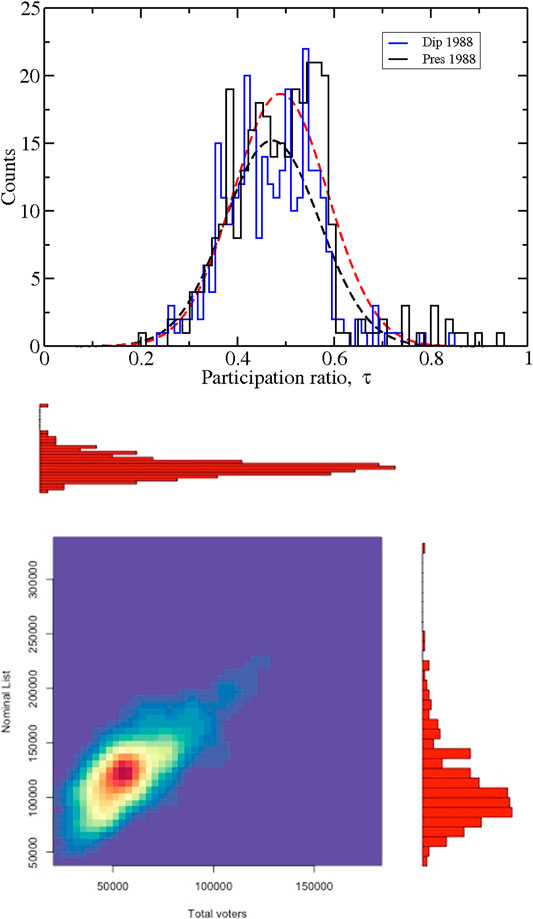
FIGURE 1. In the upper panel, we present the participation ratio, τ, for the deputies (blue histogram) and presidential case (black histogram) for the 1988 election for the 300 districts. The normal fitting appears for each case as the broken line. In the lower panel, as a heat map, the distribution of Nominal List and the total number of voters of the presidential election are presented. The corresponding histograms appear at the right and top. We use the official results published in Dictamen del Colegio Electoral (1994) for the number of votes and the data for deputies published in Centro de Estudios de la Democracia y Elecciones (1991) for the Nominal List. The later number was one of the reasons (among many others) that the 1988 election was considered rigged. So, the results for president are an approximation and for the presidential case is an exercise. Refer to text for details.

It is clear that there exist correlations between the sample size and the allowed participants, even following the rules. Hence, the goal of the present work is to show how “simple” correlations provoke deviation from the Gaussianity or the law of the large numbers. As we shall see, the correlations come from the geopolitical structure of the Nominal List. We use the dataset of federal electoral turnout of recent elections in Mexico. Such datasets are reported at the polling station aggregation level. Hence, we first describe the distribution of the sample size. For many years and through several works, such a probabilistic object was considered as a constant or, in the worst of the cases, as an asymmetric peak distribution, no matter if it is a Gaussian or Lorentzian, but we assumed a strongly peaked function around the maximum value accepted by the electoral authorities of 750. Such an assumption is false as we shall see in Section 3.1. The consequences of that are explored in the rest of the article. Previous to that, we describe the game field in the next section.

2 Materials and Methods

The datasets we consider are those published by the electoral authorities, the Instituto Nacional Electoral (INE) or its previous version, the Instituto Federal Electoral (IFE), in the official web pages (INE, 2019; IFE, 2014) consulted recently or in previous years. For a standardized version, we downloaded data from the atlas on electoral results (ATLAS, I. N. E., 2016) for the final results, called conteo distrital or districtal counting. These data correspond to the reviewed results with the political parties and include revision of anomalies reported to the electoral authorities. We considered only federal elections and no local ones; hence, our results concern about national events and with a major interest between the electorates. Datasets from 2006 federal election were compared with old files downloaded by the author during the year 2006.

The recent versions of datasets are in comma-separated values format (csv); hence, it is easy to use R or awk and sed software to clean and submit them to analysis. Older versions could be in Excel (XML) format or worse. For any dataset, a clean process is required and a record of the changes performed is considered.

The electoral distribution has several levels of aggregation, the larger level corresponds to the 300 districts corresponding to the representatives at the low chamber. They must be distributed in electoral sections, each of them with a prescribed amount of electors. The polling stations are splitted up in subsidiary ones, distributed according to the first family name; hence, the main station contains the register of those whose name starts with A up to I, for instance. The “contigua 1” or C1 admits to vote those with family name starting with H–M and so on and so forth. Each station has its list and its cabin but shares the same location, a schoolyard to say. In the dataset, each line corresponds to a poll, no matter if it is the main or the subsidiary. This alphabetical order is of procedural nature, and it does not correlate with sociodemographic variables. Hence, it is expected that considering the precinct does not change the statistics.

Each entry in the recent dataset contains the number of allowed voters in each electoral cabin; it is called the Lista Nominal or Nominal List (NL). Here, we refer to it as the number of allowed voters for the particular election. Such a number was not reported in dataset elections before year 2006. That is the reason why we considered only the last three presidential cases. Additionally, the record includes the special cabins, devoted to valid electors in transit, since they do not have a list and do not know in advance who will vote there. In the dataset, the entry devoted to the NL entry is empty. In all the data files, the field appears empty, and the R selection with the na.omit(y2) option is used. However, for Deputies 2015 (Diputado MR 2015), President 2006 (Presidente 2006), and 2012 (Presidente 2012), the field appears with a value of zero. Anyway, they are not considered for the participation ratio. The statistical analysis is performed using R and Fortran code.

3 Results

The existence of stylized facts in Mexican elections is well established (Borghesi et al., 2012; Hernández-Saldaña, 2013). The origins of them are not well understood, and many of them represent deviations from the large number theorem and are part of the richness in a complex process. Some considerations can help to understand them and cast some light on how we count and how we consider the errors. In the current work, we analyze the voter participation and voter turnout or participation ratio and how they are influenced by the geopolitical configurations of the maximum number of allowed voters in each polling station, named the Nominal List (NL). Hence, we present in the next subsection the distribution of this quantity. In Section 3.2, we shall discuss how the group conformation in the electoral process distorts the voters’ distribution, and in Section 3.3, we shall discuss the participation ratio distribution.

3.1 The Zones in the Nominal List

As mentioned before, the Nominal List (NL) or Lista Nominal for its Spanish denomination is the official record of all the citizens allowed to vote in a particular election, and a particular polling station is assigned to the voter according to its residence place. The electoral map is divided into sections with 100–3,000 electors in accordance with the law (LEGIPE, 2019), and they must fit the 300 low chamber sits. However, a uniform distribution in a heterogeneous country such as Mexico is a difficult task. The last redistricting process (2006 and 2012) was performed using a simulated annealing algorithm in order to optimize the number of possible voters in each precinct. In addition to the simulated annealing, a bee swarm strategy was applied for the 2018 election (Gutiérrez-Andrade et al., 2019). As we shall see below, the result represents an improvement in the uniformity of polling stations in the country. The main goal with this process is to avoid gerrymandering and other political skews. In this section, we show how the zones appear in the district count files for several elections; next, we analyze the effect of it on two statistics: the distribution of vote and the participation ratio or voters’ turnout, both per cabin.

Previous analysis (Hernández-Saldaña, 2009; Hernández-Saldaña, 2013) considered that the Nominal List in each polling station is conformed for around 750 registered voters. Some small deviations could be expected with an asymmetrical Gaussian or a one-sided Lorentzian distribution, for instance. However, this is not the case and we correct this assumption in this section. We focus on the last three presidential elections, but the same happens with both chambers’ elections, since the Nominal List is the same. For the local elections, the administration is different and requires a special analysis in each state.

In Figure 2A, we show the distributions of the number of registered voters in the Lista Nominal or Nominal List (NL), in each polling station from the registers in presidential elections from 2006 to 2018. The figure is drawn with lines. The black lines represent the presidential election of 2006, the blue lines represent the corresponding list to 2012, and the red lines represent the last case, 2018. The graph corresponds to a point for each value in the Nominal List; hence, we plot how many cabins have 750 registered voters, how many have 749, and so on and so forth. The first thing to notice is the existence of three windows instead of a highly concentrated asymmetric distribution before and in 750 voters. We label them as $\left(I\right)$, $\left(II\right)$, and $\left(III\right)$ containing the registers between 501 and 750, from 376 to 500, and from 1 to 375, respectively. In Figure 2B, a closeup of the region $\left(I\right)$ is presented; there is a possible new zone ranging from 501 to 560, but we enclosed all in a single region since the number of polling boxes is near to the average of the window.

FIGURE 2

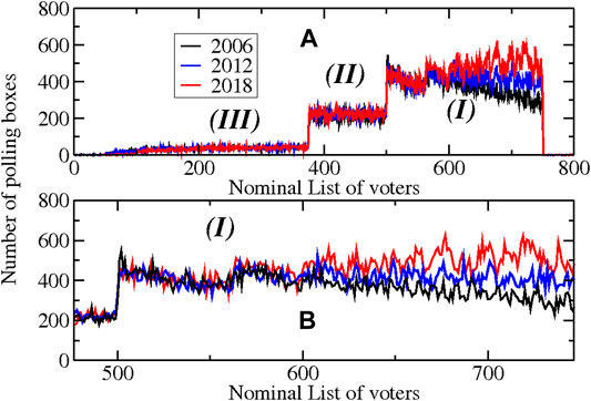
FIGURE 2. (A) Number of polling boxes with a certain number of voters in the Nominal List (NL) for the presidential elections 2006 (in black lines), 2012 (in blue), and 2018 (in red). As can be seen, they present at least three zones with jumps at 375 and 500. We named $\left(I\right)$ the region with NL between 501 and 750, $\left(II\right)$ if the NL value is between 376 and 500, and $\left(III\right)$ for the values smaller than 375. (B) A closeup to the region $\left(I\right)$ where there is the possibility that a new zone exists between 501 and around 560. Notice that the graphs present a trend.

The region $\left(I\right)$ contains 72% of the total possible voters during the 2006 election, 20% in the region $\left(II\right)$, and zone $\left(III\right)$ contains 8% of the cabins. For the 2012 process, the (rounded) numbers are $\left(I\right)$ 73%, $\left(II\right)$ 19.6%, and $\left(III\right)$ 7.52%. The presidential election of 2018 has $\left(I\right)$ 75.84%, $\left(II\right)$ 17.88%, and $\left(III\right)$ 6.28%. The existence of these distributions is the result of the electoral authorities’ decisions on a very complex problem in a very complex country, not only demographically but also geographically as well, see the work by Gutiérrez-Andrade et al. (2019). We do not disentangle the special cases devoted to the native deserved districts, so we are analyzing the statistical properties of the voters and Nominal List regardless of the geopolitical distribution, neither its urban nor its nonurban character. These possible voters’ distributions include the political parties’ requirements as well.

We notice two other features in Figure 2B: for the region $\left(I\right)$, the histogram decays for the 2006 and 2012 election; meanwhile, for the 2018 case, the distribution increases the number of cabin with almost 750 registered voters. We assume that this behavior is a result of redistricting of the 2015 process, performed by and reported in Gutiérrez-Andrade et al. (2019). Since the role of these step functions is important for the lack of Gaussianity, we tested their correlations with the other aggregation scales, the districts and the sections, but we did not find a clear correlation to the districts since we have all the values scattered in each of the 300 electoral districts for zones $\left(I\right)$ and $\left(II\right)$, representing more than 90% of the polling stations.

It is important to notice that the goal of the redistricting process is to put in a homogeneous situation all the geoeconomical regions, regardless of the urban or nonurban classification and the political party that is preponderant. The exception is the communities with a majority of Native Americans (in the continental sense, not the United States meaning).

3.2 The Distribution of Total Number of Votes

As discussed before, we shall explore the consequences of the NL stratification. Hence, we proceed to analyze the distribution of voters in each polling box, that is, the total number of voters that participate in an election. In Figure 3, we present the histogram of the distributions for the three presidential elections, normalized to the total number of participants, that is, the total sum of votes is different in each case. In black, we present the distribution for all the polling boxes. As can be seen in all the cases, the Gaussianity is not fulfilled. A shoulder appears in the left side of the distributions. However, if we separate the results according to the allowed amount of voters in each box, that is, the Nominal List, an explanation emerges. The left shoulder is composed of the polling stations with few registered voters. That is what we call zone $\left(III\right)$, and this happens in the three cases, the distributions appear in blue. Since the corresponding distributions for zones $\left(I\right)$ and $\left(II\right)$ have, practically, zero participation in the shoulder, the zone $\left(III\right)$ explains it. The distributions of votes for district or municipality are unable to explain the shoulder.

FIGURE 3

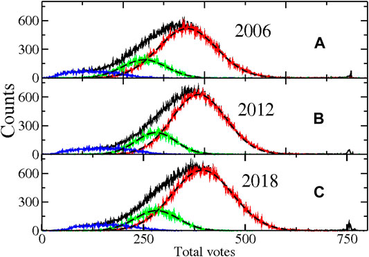
FIGURE 3. Distribution of total votes for the presidential turnout of 2006 (A), 2012 (B), and 2018 (C) normalized to the total number of valid votes in each process. In black line, in all the panels, the distribution corresponds to the whole election. In red, the corresponding distribution is plotted if we consider votes that come from polling stations with a Nominal List between 501 and 750, named $\left(I\right)$ in Figure 2; in green, those from $\left(II\right)$; and in blue, those coming from stations with a Nominal List number smaller than 375. In the broken black line appears a Gaussian fitting for distributions in zones $\left(I\right)$ and $\left(II\right)$.

Since we explained the shoulder origin, we focus on the properties of the distribution for the zones $\left(I\right)$ and $\left(II\right)$. They are well-behaved distributions with a Gaussian look. However, as it is usual, if a distribution is or not a Gaussian is hard to say (see, for instance, Székely and Rizzo (2005) and references therein). In the present work, we do not discuss it; we concentrate on the properties of the distribution that arose from considering the total votes for each specific NL value for zones $\left(I\right)$ and $\left(II\right)$. The first three statistical moments are a smooth function with fluctuations if we consider them in terms of the Nominal List. The averages are well adjusted by a linear function, as shown in Figure 4A. The slope is smaller for the zone $\left(I\right)$ than the others, but it remains linear. The standard deviation (SD) is linear in the vast majority of values of NL, with an increase as NL reaches the limit of 750, as appears in Figure 4B. The skewness has large fluctuations but almost all the distributions for zone $\left(I\right)$ and $\left(II\right)$ are negative; it is plotted for the three cases in Figure 4C. We tested, with a positive result, on a sample of ten distributions along the zone $\left(I\right)$ values in order to recover the normal-like shape, as shown in Figure 3. That is, a central limit theorem holds. The consequences of these dependences are left to an ulterior analysis.

FIGURE 4

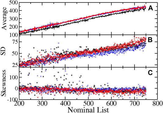
FIGURE 4. In (A), we plot the average number of voters participating in each polling station as a function of the Nominal List for the presidential elections for 2006 (black), 2012 (blue), and 2018 (red). The relation is linear in all the described zones, but the slope is smaller for zone $\left(I\right)$. The standard deviation is shown in (B). It is linear with a change in the tendency near NL = 750. The skewness is shown in (C); it presents large fluctuations, but the vast majority of cabins in zone $\left(I\right)$ present a negative value. In (B,C), the black circles correspond to 2006, the blue squares to 2012, and the red down triangles to 2018.

Additionally, in Figure 3, we show the result for the special polling boxes for the overall case; they appear as the distribution fluctuations for values around 750 votes (the small peaks around that value). In the registers, these polling stations appear with zero allowed voters since they are devoted to persons in transit. Notice that if the number of persons allowed to vote in these cabins is set to 750 or so, they will appear as an extramaximum in the participation ratio around unity. Such suspicious distributions have been assumed as a signature of manipulations. Two examples with a considerable deviation are the Mexican elections in 1988 (Barberán et al., 1988; Auping-Birch, 1988) and the Duma elections in Russia in 2011 (Neretin, 2012), where large peaks appeared. Hence, a clear identification of those special cases in the database is important. For a more recent and available reference for the Mexican scenario, see López-Gallardo (2018), where some of the graphs from Barberán et al. (1988) are reprinted. The votes from registered citizens in foreign countries are considered neither in these analyses nor in the current work.

3.3 The Participation Ratio

In the literature, the participation ratio is an important quantity to be analyzed. It is defined in Eq. 1 as ${\tau }_i=\frac{{\upsilon }_i}{N_i}$, where ${\upsilon }_i$ is the number of voters who deposited their votes in the polling station i with a Nominal List of $N_i$. As there are many ratios in statistical analysis, it is assumed that it follows a Gaussian distribution. However, the distribution over the nationwide registers is not a Gaussian in the three elections considered here. They correspond to an asymmetrical single maximum distribution. It resembles a normal distribution, but the asymmetry is clear. To consider a Gaussian approximation for the distribution of t is a good starting point for much more complex calculation, such as the diffusion-like equation for the intention field proposed by Borghesi and Bouchaud (2010). However, even in this reference, the distribution of a related quantity, named

$\begin{array}{l}^\eta =\frac{N_{+}}{N_{-}}\\ ^\eta =\frac{\tau }{1-\tau }\end{array}(2)$

is not Gaussian. In Eq. 2, $N_{+}$ is the number of participating voters and $N_{-}$ labels the nonparticipating ones. Since $N=N_{+}+N_{-}$, we obtain the second line in Eq. 2 and we discard the aggregation level. In reference (Borghesi and Bouchaud, 2010), the level of aggregation is larger than the current work, but a similar calculation gives similar results for the Mexican case (figure is not shown). Hence, violation of Gaussianity is not a necessary feature of election manipulation.

In Figure 5, we plot the distribution of $\tau ,P\left(\tau \right)$, normalized to one, for the three elections. In Figure 5A, the distribution is built up using all the data, except those corresponding to special polling stations and votes from outland. As can be seen, the distribution is not a Gaussian. In order to make it evident, we plotted in a semilog scale. The result is not better when we use only the polling states in zone $\left(I\right)$ or in zone $\left(II\right)$, where a Gaussian behavior has been claimed for the distribution of vote. Deviations using the window $\left(III\right)$ are not surprising, with larger deviates, and are not shown.

FIGURE 5

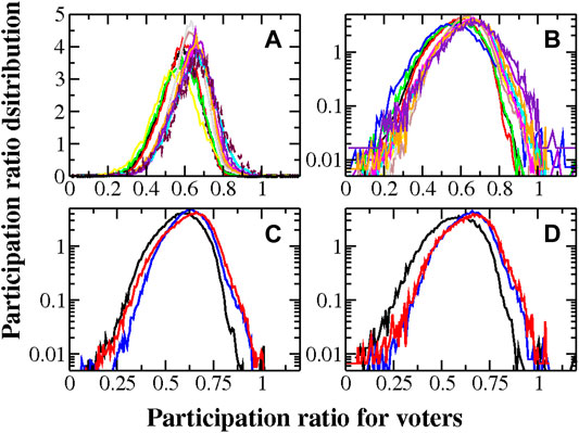
FIGURE 5. Distributions of the participation ratio of voters, τ, for the presidential elections are plotted. In (A), all the cases are presented, considering all the valid voters and regular cabins and the ratio of the zones $\left(I\right)$ to $\left(II\right)$ for the elections considered. In order to notice the lack of Gaussianity, the same graph is plotted in a semilog scale in (B). In (C,D), the distribution for zones $\left(I\right)$ and $\left(II\right)$ for the 2006 (in black), 2012 (in blue), and 2018 (in red) elections is presented.

In an homogeneous scenario, where (almost) all polling states have a unique number of allowed voters, the Gaussianity in the distribution of voters is reflected in the Gaussianity in the participation ratio, since ${\tau }_i$ is a scaled variable, say ${\tau }_i={\upsilon }_i/N$, with N fixed. In such a case, if the distribution of votes is a Gaussian, so is the ratio with the Nominal List.

However, as explained in Section 3.2, the distribution of allowed voters is not so simple. Even more, from Figure 2, the Nominal List is distributed within windows with fluctuations around an average, from around 400 in zone $\left(I\right)$ and 200 for the window $\left(II\right)$, but even there they have a trend with negative slope for 2006 and positive for the 2018 case. So, the participation ratio distribution $P\left(\tau \right)$ is the distribution of the ratio of two correlated variables. As can be seen in Figure 4, the average of vote distribution is linear in zones $\left(I\right)$ and $\left(II\right)$ with no large deviation, but the same is not true for the standard deviation and superior moments. The skewness is negative for almost all the distribution in zone $\left(I\right)$ but is not clear if there exists a functional relation with the NL.

In Figure 6, the heat map is plotted for the election of 2018; it represents the total vote as function of the Nominal List. It shows that the number of voters in the tally is not larger than the registered ones. The function seems to be linear but with large fluctuations and scarce of data for small values, there are votes in all polling stations. This behavior is seen in Figure 4, with near to linear standard deviation and negative skewness, as explained in the previous section. In the last section in the heat map, where the NL is near to 750, the fluctuations are larger and the standard deviation is no longer linear. The behavior is similar for all the considered cases, including the controversial election of year 2006.

FIGURE 6

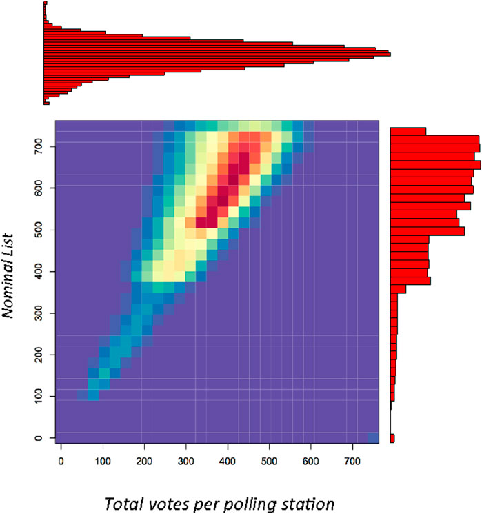
FIGURE 6. Heat map of the total number of votes per polling station and Nominal List for the 2018 presidential election: the color code starts in blue for zero values and ends in red for increasing values. In the upper part, distribution of total votes which appears in Figure 3C as black line is presented. At the right, the Nominal List histogram is given, a detailed view appears in Figure 2.

The analytical form of the joint distribution probability distribution is hard to achieve, mainly, since the distribution in the denominator of t is not a step function. Hence, in order to obtain some insight, we proceed to consider an ensemble of distributions for each value in the Nominal List $N=\kappa$. So, we build up the distribution of each ratio ${\tau }_{\kappa \text{,i}}={\upsilon }_i/\kappa$; we call such a distribution as $P_{\kappa }$. A calculation like this is feasible since zones $\left(I\right)$ and $\left(II\right)$ have hundreds of data, around 400 for the former and 200 for the later for each value in the List. Each distribution $P_K=\left(\tau =\upsilon /N|N=K\right)$ has measurable moments, and we try to elucidate if they correspond to a simple distribution. Of course, if the distributions are Gaussians, the resulting distribution from the sum of all the variables is a Gaussian.

The skewness for the vast majority of the cases is negative and concentrated around a value. Hence, a graph of all the $P_{\kappa }$’s must correspond to a skewed left PDF. In Figure 7, we show the result for the standardized variable ${\eta }_i=\left({\tau }_{K,i}-<{\tau }_K>\right)/{\sigma }_k$ for the zone$\left(I\right)$ of the 2018 election. The other datasets considered in this work have a similar behavior, but we left this single case in order to be clear. In blue circles appear the distributions of η. However, the skews in Figure 4C and the quadratic falls in Figure 5 in the semilog scale suggest a skewed Gaussian, with explicit form

$\prod \left(x\right)=\frac{1}{\sqrt{2\pi \omega }}\exp \left(-\frac{{\left(x-\xi \right)}^2}{2{\omega }^2}\right)\left(1+erf\left(\alpha \left(\frac{x-\xi }{\omega }\right)\right)\right)(3)$

where $\text{erf}(\cdot )$ is the error function (O’Hagan and Leonard, 1976; Azzalini, 1985). The fitting from this function to the data is shown as the black line in Figure 7. The fitting for the other cases is similar and not shown. Even when the fit looks fine, the deviations at the tails are noticeable, even in the linear scale. The differences between the histogram and the fitted function for values of $\left|\eta \right|>3$ are larger. So, the fitting does not pass the Kolmogorov–Smirnov test but is a good guide for the kind of effect caused by the finite size of the Nominal List. Notice that this effect is not as simple as a cut in the distribution; the mode is consistently larger than the mean. In the next section, we propose a mechanism to fit the distribution with one single parameter, the correlation between the participation ratio, and the difference between the Nominal list and the number of voters. Such a model is depicted as the broken black line in Figure 7.

FIGURE 7

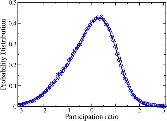
FIGURE 7. Distribution of the normalized participation ratio, $\eta =\left({\tau }_{\kappa }-{\langle \tau \rangle }_{\kappa }\right)/{\sigma }_{\kappa }$, for the 2018 election and zone $\left(I\right)$, in blue dots with lines. The black line corresponds to a fitting for the data using a skewed Gaussian, given by Eq. 3. The broken black line corresponds to the same distribution but ruled by the single parameter related to the correlation between the participation ratio and the difference of the Nominal List and the number of voters, properly standardized. See the discussion, in Section 4, for explanation. The shift of the theoretical curves is around 0.08.

Another aspect to consider is the form of the individual distributions for each NL value. Even if they are skew normal functions, the sum of them is neither Gaussian nor skew normal. In a closed form is the sum of Gaussian and a finite sum of functions that involve the Kampé de Fériet function (Nadarajah and Li, 1985).

4 Discussion

The return of physicists to analyze the complexity of social and economical behavior came with the use of simple models. However, simple models not always mimic the nature of the systems. Two common places describe such a point of view: 1) the Markovian elector and 2) the large number law for elections. It is a fact that electors have memory; if the people forgot something, the parties are there to remember it. The violation of the second is sometimes the reason to call for a violation of the electoral system. However, as the present work pretend to show, correlated variables give place to apparent violations of the law. For instance, in a recent study (Peters, 2019), the author focused on a problem of assuming ergodicity in economics; meanwhile, economics is a time-dependent system by excellence. Hence, the author claimed that a reconsideration of the use of ergodicity in economics could explain some puzzles. Thus, complex systems present complex behavior, no matter if we understand the cause or mechanism. The existence of stylized facts in electoral systems is the evidence that no particular phenomena occur in the system and their interrelationships. Hence, a careful analysis of the database and the conditions is required.

Statistical analysis assumes that in a random process, the proportion of positive events to the total number of events is a random variable with Gaussian distributions if we consider a large number of events. For a not-so-large number, it could be deviations or approximations, for instance, a binomial distribution that approaches a Gaussian for large number of experiments. However, Mexican electors, as the vast majority of the electors, are not balls in the Bernoulli experiment. As shown in Figure 2, the sampling could be tricky, even when the electors have a Gaussian distribution.

As shown in Figure 3, disentangling the NL by zones explains the shoulder in the distribution of voters. Only the zone $III$, with few registered voters per cabin, does not follow the normal behavior. This shoulder was characterized as an anomaly in Román (2006) for the 2006 election but finds an explanation in the NL stratification. The other distribution analyzed here was the participation ratio of voters that in López-Gallardo (2018) is considered a Gaussian and contrasted with non-Gaussian behavior of other variables. However, as shown in this work, it corresponds to a nonsymmetrical Gaussian, near a skew normal.

The distributions of the several cases analyzed here show that the distortion is not simply a cutoff of the sample size. In Figure 7, we fitted a skewed Gaussian to the standardized participation ratio, η, where the mode is larger than the mean. Hence, instead of having a Gaussian distribution with a truncated tail, we have a distorted Gaussian due to the existence of a constraint. A way to explain the skewed distribution for τ and η is considering a truncation process. In Azzalini and Valle (1996), a mechanism of hidden truncation is used to obtain a skew normal function (see Arnold and Beaver (2002) and references therein). They consider a process where the accepted values must be above a certain limit. The argument is presented as a proposition in there, and it is as follows: consider a couple of random variables $Z,Y$ with a standardized normal bivariate distribution. The variables have a correlation δ. The conditional probability of Z given that $Y>0$ is

$P\left(Z\le z|Y>0\right)=\frac{P\left(Z\le z,Y>0\right)}{P\left(Y>0\right)}(4)$

$=2P\left(Z\le z,Y>0\right)(5)$

where the second line comes from the fact that Y is standardized. Without lack of generality, the relation of Y and Z can be written as

$Y=\delta Z-\sqrt{1-{\delta }^2}W(6)$

for Z and W i.i.d. variables. Since $Y>0$, it implies that $\delta Z-\sqrt{1-{\delta }^2}W>0$ or $\delta Z/\sqrt{1-{\delta }^2}>W$. Under such assumptions, $P(Z\le z|Y>0)$ is skew normal. The skew factor is

$\alpha =\delta /\sqrt{1-{\delta }^2}(7)$

In the current case, we consider the requirement that $Y>0$ for the difference $\varphi =N-\upsilon >0$ and, properly standardized, we shall call it ψ. We use a different variable since ψ and η do not follow a normal bivariate distribution. The condition $\psi >0$ implies that

$\frac{\delta }{\sqrt{1-{\delta }^2}}\eta >W(8)$

if the variables are related as in Eq. 6. Under the conditions considered by Azzalini and Valle (1996), η has a skew normal distribution. Since the only free parameter is $\delta =corr\left(\psi ,\eta \right)$, we plot a skew normal with shape parameter α as in Eq. 7. The value of δ is ${\delta }_I\approx -0.933978$ for the 2018 election and zone I. The skew normal distribution with this single parameter is depicted in Figure 7 as the broken black line. The value of the correlation, ${\delta }_I$, fixes the other parameters since the mean is zero and the SD is 1. The function is shifted from the histogram by an amount of around 0.08. In order to understand how relevant the shift is, we use the parameter values of the skew normal fitted (black line in Figure 7) and calculate the correlation value corresponding to the fitted one. Such a value is $-0.932961$, with an absolute difference of 0.001 with ${\delta }_I$. We obtained the value of δ using the relation $\omega =\delta /\sqrt{1-2{\delta }^2/\pi }$. Notice that the variables $\psi =N-\upsilon$ and $\tau =\upsilon /N$ do not have a normal bivariate distribution.

5 Conclusion

In this work, we deal with the distribution of the official list of allowed participants in a given election, named Nominal List (NL) or Lista Nominal in Spanish. The number of voters is previously designed (see Gutiérrez-Andrade et al. (2019)) with considerations to avoid gerrymandering and other influences from the political parties. Here we found that the number of voters is distributed according to zones resembling step functions (see Figure 2). The three zones were explicitly marked, with zone $\left(I\right)$ being the most populated and zone $\left(III\right)$ being the less crowded. The consequences in the distribution of votes and the participation ratio are analyzed considering this finding at a degree of aggregation of polling station. The distribution of votes presents a shoulder in all the elections when all the cabins are considered. However, this shoulder is explained by scrutiny of the number of possible participants in the elections according to the zone. The disentangle of votes according to the zones allows us to explain the shoulder: it corresponds to the less populated cabins and certainly contributes with fewer votes to the overall count (see Figure 3). The separated distributions of the other zones recover a Gaussian-like shape, as expected by the large number theorem, even when the individual distributions are not Gaussian.

However, it is clear that there exist correlations between the distribution of voters and the NL. The average of the number of voters participated in each station grows linearly with NL, as shown in Figure 4. This conditioned the behavior of the participation ratio distribution, considered as the turnout distribution at a polling station degree of aggregation. For this quantity and the standardized variable, we obtain a near to skew normal function, with deviations at the wings, as shown in Figure 7. The analysis was performed for the most populated zones.

Even the disentangled zones are able to explain the asymmetry in the distribution of the standardized participation ratio. Such a distribution could be compatible with a skewed Gaussian function, as showed in Figure 7. The complicated constraint of the Nominal List (NL), shown in Eq. (2), gives a similar distribution for all the cases analyzed.

Beyond the actual distribution followed by the participation ratio of voters, the skewed Gaussian appears consistently in all the cases, regardless of the geopolitical or economical situation, neither its urban nor nonurban condition. So, the standardized participation ratio of voters could have a generic distribution, like the skewed Gaussian. A way to introduce the relation of the Nominal List (NL) and the number of voters, v, is through the constraint $N-\upsilon >0$ and the participation ratio $\tau =\upsilon /N$ of the conditional probability given in Eq. 4 for variables properly standardized that correspond to a skew normal. This mechanism explains the asymmetry and the bulk part of the distribution. The analysis of the tails is a matter of current analysis.

A final remark is that no priori assumptions must be taken when handling truly complex systems, such as the electoral processes.

Data Availability Statement

The datasets generated for this study are available on request to the corresponding author.

Author Contributions

HH-S conceived the paper, cleaned the data, coded the programs, and wrote the paper.

Funding

PRODEP-SEP support through Programa de Apoyo para el Fortalecimiento de los Cuerpos Académcos. The author is a member of the Cuerpo Académico Física Teórica y Materia Condensada. Divisional project CBI, CB008-13, Universidad Autónoma Metropolitana at Azcapotzalco, gave support.

Conflict of Interest

The author declares that the research was conducted in the absence of any commercial, financial or political relationships that could be construed as a potential conflict of interest.

Acknowledgments

The author thank H. Várguez and E. Várguez for their kindness during the time this work was in progress.

References

Arnold,, B. C., Beaver, R. J., Bhaumik, A., Dey, D. K., Cuadras, C. M., Sarabia, J. M., et al. (2002). Multivariate models related to hidden truncation and/or selective reporting. Test 11, 7–54. doi:10.1007/bf02595728

CrossRef Full Text | Google Scholar

ATLAS, I. N. E. (2016). Sistema de consulta de la estadística de las elecciones federales 2014-2015/atlas de resultados de las elecciones federales 1991-2015. Mexico: Instituto Federal Electoral.

Auping-Birch,, J. (1988). Elecciones federales de México: julio de 1988: interpretación de los resultados oficiales mediante el análisis matemático. Mexico: IEES.

Azzalini,, A. (1985). A class of distributions which includes the normal ones. Scand J. Statist. 12. 171–178. doi:10.6092/issn.1973-2201/711

CrossRef Full Text | Google Scholar

Azzalini,, A., and Valle, A. D. (1996). The multivariate skew-normal distribution. Biometrika 83, 715–26. doi:10.1093/biomet/83.4.715

CrossRef Full Text | Google Scholar

Ball,, P. (2004). Critical Mass. New York: Farrar, Straus and Giroux.

Baltz,, S., McAlister, K., Pineda, A., Vasselai, F., and Mebane, W. (2018). “Agent-based models of strategic electoral behavior in election forensics,” in Annual Meeting of the Midwest political science association, Chicago, IL, November 22.

Google Scholar

Barberán,, J., Cárdenas, C., Mojardín, A. L., and Zavala, J. (1988). Radiografía del fraude: análisis de los resultados oficiales del 6 de julio. Mexico: nuestro Tiempo.

Borghesi,, C., and Bouchaud, J. P. (2010). Spatial correlations in vote statistics: a diffusive field model for decision-making. Eur. Phys. J. B 75, 395–404. doi:10.1063/PT.3.384510.1140/epjb/e2010-00151-1

CrossRef Full Text | Google Scholar

Borghesi,, C., Raynal, J. C., and Bouchaud, J. P. (2012). Election turnout statistics in many countries: similarities, differences, and a diffusive field model for decision-making. PLoS One. 7, e36289. doi:10.1371/journal.pone.0036289

PubMed Abstract | CrossRef Full Text | Google Scholar

Cantú,, F. (2019). The fingerprints of fraud: evidence from Mexico's 1988 presidential election. Am Polit Sci Rev. 113, 710–26. doi:10.1017/s0003055419000285

CrossRef Full Text | Google Scholar

Centro de Estudios de la Democracia y Elecciones (1991). Cede laboratorio de análisis político y políticas públicas, base de datos. Mexico City: UAM Iztapalapa.

Dictamen del Colegio Electoral (1994). “Declaratoria de Presidente Electo de los Estados Unidos Mexicanos al Licenciado Carlos Salinas de Gortari para el periodo 1988-1994 emitida por la Cámara de Diputados de LIV Legislatura, erigida en Colegio Electoral,” in Elecciones a Debate 1988: las actas electorales perdidas. EditorsA. S. Gutiérrez (Mexico: Diana).

Google Scholar

Gutiérrez-Andrade,, M. Á., Rincón-García, E. A., de-los-Cobos-Silva, S. G., Lara-Velázquez, P., Mora-Gutiérrez, R. A., and Ponsich, A. (2019). Simulated annealing and artificial bee colony for the redistricting process in Mexico. Inform. J. Appl. Analytics. 49, 189–200. doi:10.1287/inte.2019.0992

CrossRef Full Text | Google Scholar

Hernández-Saldaña,, H. (2009). On the corporate votes and their relation with daisy models. Physica A Stat. Mech. Appl. 388, 2699–704. doi:10.1016/j.physa.2009.03.016

CrossRef Full Text | Google Scholar

Hernández-Saldaña,, H. (2013). Result on three predictions on july 2012 federal elections in Mexico based on past regularities. Plos ONE. 8, e82584. doi:10.1371/journal.pone.0082584

PubMed Abstract | CrossRef Full Text | Google Scholar

IFE, (2014). Instituto federal electoral web page.

INE, (2019). Instituto nacional electoral web page.

Klimek,, P., Yegorov, Y., Hanel, R., and Thurner, S. (2012). Statistical detection of systematic election irregularities. Proc. Natl. Acad. Sci. U.S.A. 109, 6469–16473. doi:10.1073/pnas.1210722109

PubMed Abstract | CrossRef Full Text | Google Scholar

LEGIPE, (2012). Compendio de Legislación nacional electoral. Tomo II. Mexico: Instituto Nacional Electoral.

López-Gallardo,, J. A. (2018). Basta de Fraudes Electorales 1988-2018. Mexico: Plaza y Valdés.

Mebane,, W., and Jackson, J. E. (2014). “Preference heterogeneities in models of electoral behavior,” in Annual Meeting of the Midwest political science association, Chicago, United States, April 3–April 6, 2014.

Google Scholar

Nadarajah,, S., and Li, R. (1985). The exact density of the sum of independent skew normal random variables. Scand. J. Statist. 12:171–178. doi:10.1016/j.cam.2016.06.032

CrossRef Full Text | Google Scholar

Neretin,, Y. (2012). On statistical researches of parliament elections in Russian federation. NY: Cornell University arxiv.

O’Hagan,, A., and Leonard, T. (1976). Bayes estimation subject to uncertainty about parameter constraints. Biometrika 63, 201–203. doi:10.1093/biomet/63.1.201

CrossRef Full Text | Google Scholar

Ortega,, R. Y. (2017). Presidential elections in Mexico: from Hegemony to Pluralism. Cham (Switzerland): Springer International Publishing.

Peters,, O. (2019). The ergodicity problem in economics. Nat. Phys. 15, 1216–1221. doi:10.1038/s41567-019-0732-0

CrossRef Full Text | Google Scholar

Román,, C. M. R. (2006). Simulación por computadora del fraude electoral. Mexico City.

Schweitzer,, F. (2006). Sociophysics. Phys. Today. 71, 40. doi:10.1063/PT.3.3845

CrossRef Full Text | Google Scholar

Székely, G. J., and Rizzo, M. L. (2005). A new test for multivariate normality. J. Multivariate Anal. 93, 58–80. doi:10.1016/j.jmva.2003.12.002

CrossRef Full Text | Google Scholar