Assessing and Modelling Tail Dependencies Between Service Times in Discrete Event Simulation With Minimum Information Copulas for a Better Understanding of Maximum Time in System Risk

1 Introduction

In the mathematical modelling literature and practice, Discrete Event Simulation (DES) is a well-established method for analysing dynamic, stochastic and complex real-world problems. It is applicable whenever a system can be represented by events occurring over time and thereby changing the system’s state. Between these events no changes to the system’s state occur. Common applications simulate manufacturing, healthcare and call-center processes for which main events are i.a. arrivals of entities, such as product parts, patients and calls entering a simulated system, as well as them being serviced by servers, e.g. being processed by machines, attended by clinicians for physical examinations or answered by call-center agents. Usually, entities queue between different steps of a process whenever servers are busy or unavailable. See Robinson [1] for an extensive introduction to DES.

DES models’ main input parameters, the inter-arrival time distributions between incoming entities and the service (or processing) time distributions of servers, are often modelled assuming independence. For service times this applies for both, times of successive entities at a server and timing distributions across multiple, different servers. This modelling choice might stem from modellers’ preference for certain univariate parametric input distributions, perhaps for simplicity or due to experience from similar simulation projects, or this choice is based on observations. In the latter case, independence is either indeed a sensible assumption (based on the observations) or insufficient data is collected for determining dependence relationships. However, unless justified by sufficient observations, ideally together with other evidence, such as specifications made in the conceptual modelling phase (the decision or abstraction process of what to include in a simulation model [2]), independence can be an oversimplified assumption for understanding a system’s risks properly. In DES, such risks refer for instance to increased queue lengths (and waiting times) due to dependent arrivals or little throughput from a process due to dependent long service times. A result of interest in many DES applications, which can be affected significantly by dependencies, is maximum time in system. It captures the maximum time to complete the simulated process across all entities. Closely related and hence also possibly impacted by potential dependencies are results capturing the percentage of entities needing longer than a certain threshold to complete a process.

In this paper, we consider service time dependencies and their impact on the maximum time in system and related results. Especially, we look at tail dependencies and extremely long service times (usually above their 90th, 95th or even 99th quantile) at one server followed by extreme service times at a different server (for the same entity). However, the methods presented here can be used also for other dependence relationships in DES, such as between times of successive entities at the same server. A main modelling challenge is the lack of relevant, historical data on these extreme service time dependencies. Thus, we focus on assessing minimum information copulas through expert judgements for specifying our service time dependencies.

The paper’s first contribution is to enhance the DES toolkit by presenting a modelling framework for including dependent tail uncertainties between service time distributions through copulas. While Taylor et al. [3] and Cheng [4] highlight the importance of considering dependencies in DES modelling as future key research area and while Biller and Ghosh [5] recognize multivariate distributions’ importance for simulation input modelling when reviewing suitable dependence models, applications including probabilistic dependencies in DES models are rare. Further, the impact of tail dependencies on model outputs and results has been neglected in the simulation literature. This is despite Cheng [4], Pasupathy and Nagaraj [6], Biller [7] and Biller and Corlu [8] mentioning copula theory’s potential for simulation modelling. Yet, with these references mainly addressing arrival processes, we aim for extending the treatment and understanding of dependencies and tail dependencies between service time distributions. Note, we focus on DES in this paper due to simulation modelling’s suitability for various complex problem situations. However, we acknowledge that dependencies between service times have been studied previously for specific queueing systems in the queueing theory literature dating back to Mitchell et al. [9] and Pinedo and Wolff [10]. The second and main contribution is to provide simulation modellers with a method for including information on detailed dependencies through expert judgements when facing a lack of relevant, historical data on these. Extreme outcomes of joint service times are only rarely observed and available in data sets which is why their inclusion in a simulation often constitutes a main modelling challenge. According to the author’s knowledge, this is the first application of assessing copulas through expert judgement in DES modelling. Lastly, we classify common sources and types of dependencies for commonly simulated systems. This classification is a novel way of structuring the related simulation literature.

The paper’s remainder is as follows. In Section 2, we present our classification of different sources and types of dependence relationships possibly relevant for DES. In Section 3, we briefly review the literature on methods assessing dependence models for the previously classified sources and types. Section 4 presents our method to assess tail dependencies between service time distributions through expert judgements. The relevant background on minimum information copulas as a suitable way for modelling tail dependencies between service times is discussed. In Section 5, we apply our method and show the impact of tail dependencies on the maximum time in system for a simple ambulance emergency simulation model. We conclude the paper in Section 6 by reflecting on our method’s achievements and outlining future research areas for copula theory and expert judgement in DES modelling.

2 Classifying Sources and Types of Dependencies in DES Modelling

In DES, several sources and types of dependent uncertainties can impact a simulation’s behaviour and results. It is worth clarifying their differences and discussing how they are dealt with in the simulation literature. Therefore, we present a classification and an overview of approaches to include them in DES models.

An early study considering dependent uncertainties in DES is Wilson [11] who includes bivariate Gaussian distributions and (as extension) bivariate Johnson distributions in a simulation. As an example he mentions a workpiece, which is being processed at various manufacturing cells, whereas a “higher-than-average” processing time at the first cell is likely to be followed by longer processing times at the later cells.

General overviews on including dependencies in simulations are provided in Biller and Ghosh [5] and Biller and Corlu [8]. The latter is of interest for us given its discussion about copulas in simulation input modelling.

With our focus on dependencies between service time distributions, we consider dependence relationship similar to Wilson [11]. Other treatments of dependent uncertainties exist in simulation modelling whereas the majority considers those between arrival rates and dependencies between inter-arrival and service times (e.g. serial dependencies or autocorrelations and dependencies across time and arrivals). However, arrival processes are out of scope here and for overviews on including their dependencies in DES, we refer to Biller and Ghosh [5] and Ibrahim et al. [12]. We only briefly mention Biller and Ghosh [13] and Channouf and L’Ecuyer [14]. The latter use Gaussian copulas for dependent arrivals in a call-center while the former model dependencies between customer arrivals and demand using Vine copulas [15].

As we clarified earlier, our DES approach in this paper is different to analytical methods in queueing theory including dependencies. When outlining the different dependence types in this section, however, we cover some examples from that research area due to a similar understanding of dependencies’ impact on systems.

2.1 Service Time Dependencies From the Number of Serviced (Processed) Entities

A first possible source for dependencies between service time distributions stems from the number of serviced (or processed) entities at servers. That is, the more entities have been processed by servers, the slower or faster their service times become. In this context, dependencies between service times arise either at the same server for each successively serviced entity or they arise for service times at different servers given that the number of entities in the system affects these in the same way.

On the one hand, we aim for including servers’ fatigue in our DES models, leading to a joint downward trend in successive service times. Thus, the service time for a specific entity is more likely to take longer given that the previous one already exceeded a certain quantile for its time distribution. On the other hand, learning effects occurring with each serviced entity can speed up successive service times [16]. In both cases, service times correlate, usually positively when experiencing the same learning or fatigue effects.

Learning and fatigue concern also the operations management literature which frequently makes use of simulation models and analytical approaches of queueing theory. Here, the idea of a system’s load often leads to successive service times being dependent [17]. Additionally to fatigue, Dong et al. [17] mention also psychological factors for service times jointly slowing down. A higher load increases pressure which in turn slows decision-making and information processing. With non-human servers, a high system load might also induce slowdowns due to technical reasons. Dong et al. [17] mention the example of slower performance of IT systems due to high load. Reasons for joint faster service times in the operations management literature are “speed-up manifests” as they apply in intensive care units, production lines and various types of service lines [18].

The number of processed entities (or load) typically depends on the incoming arrivals into a system. While, as aforementioned, the detailed discussion of arrival processes is out of scope in this paper, briefly note that capturing and fitting dependence models between arrival rates and service times has also been considered (see e.g. Brown et al. [19]). In that way, service time distributions can be related due to intra- and inter-day, but also weekly, monthly and seasonal fluctuations of arrivals. This is also termed “time-series dependence” [1].

2.2 Service Time Dependencies From Different Server Types

In other cases, possible service time dependencies stem from considering specific, different server types. At a server, we might need a human or machine who or which needs to be present for an entity to be serviced or processed. Different server types are then for instance humans with specific skill-sets or machines with different performance and quality levels. Service times, either at the same server or across different ones, are then dependent conditional on the specific server type that is doing the work there, positively if they are of the same type or negatively if they are different types.

In the broader literature on queueing systems this is often termed “heterogeneous server problem”. Armony [20] and Armony and Mandelbaum [21] mention the example of including a pool of trainees and a pool of experienced servers in a model whereas whenever the first ones are on shift, we expect joint slower service times. Optimal solutions on scheduling and staffing are proposed, often by optimising skills-based routing for heterogeneous server types. For an overview on modelling approaches to service times based on heterogeneous servers, see also Gans et al. [22].

2.3 Service Time Dependencies From External Events

Another type and source of dependent service time uncertainties is of systemic nature. That is, service times can be dependent based on events external to the modelled process. These might cause service times to jointly deviate either across different servers (each affected by the same external event) or for successive entities at the same server.

Xie et al. [23] mention two examples of dependencies in simulations that are induced by what they term “common latent factors”. As such, task durations in project planning simulations can be correlated due to factors, such as weather conditions. In production lines, e.g. of jet engines or semiconductors, the overall room temperature could impact several machines’ performance and likelihood of breakdowns. Similarly, when simulating a company’s call center, Pang and Whitt [24] consider the defect of a sold product (occurring with a certain probability) as external event that causes all calls to take longer. When modelling arrivals into an emergency call center, L’Ecuyer et al. [25] include dependent arrivals as bursts which are triggered by a single (external) emergency event, e.g. a fire, accident or terrorist attack and impact service times. In a reliability context, Wilson [11] provides a more general example in which times to failure for several servers are strongly related and tend to fail simultaneously because of a common shock to the system. These failures then affect service times for all process’ steps (servers) jointly. Finally, in a simulation of a hospital’s emergency room, multiple patients might be associated through the same medical incident. Several patients can be victims of a single highway accident or food poisoning at the same restaurant. Such common causes might lead to several service times taking longer than usual as various patients are affected by the same external event [24]. In the previous examples, service times are typically positively correlated as several servers in a simulated process need to cope with these new conditions stemming from external events in the same manner.

Note, a common way for including external events with potentially systemic impact in DES is the use of hybrid simulations. These use other simulation techniques and stochastic processes additionally to DES models to specify the occurrence of external events. Conditional on the outcome of the other model, the service time distributions in the DES are adjusted [26]. We consider the direct modelling of service time dependencies as an alternative when hybrid modelling is not possible or out of scope.

2.4 Service Time Dependencies From Entities’ Inherent Characteristics

Lastly, dependencies between service time distributions might arise due to inherent characteristics of the entities going through a system or process. For example, patients usually have different health conditions and a patient with complex conditions, who took longer in a physical exam, might also be more likely to need longer at other servers, such as the GP consultation about further steps for their treatment. Likewise, a workpiece’s specific characteristics might cause it to have longer processing times at each in a series of machining stations [11].

In another example, Stanfield et al. [27] include correlations between the operation times of items undergoing a re-use (recycling, repair or re-manufacturing) process in product-reuse production systems. Here, an item’s initial condition can be highly varied whereas jobs on items with an initial good condition are done faster at each step of the process while items in poor condition take longer for several or all tasks (servers). They propose an extension of the Johnson distribution for capturing the univariate and multivariate distributions which requires a specification of the first four moments for the marginal distributions together with the correlation matrix. The authors highlight the advantage of not having to use Gaussian marginal distributions as required for a multivariate Gaussian distribution.

A further example for this dependence type is Jaoua et al. [28] who use copulas to capture probabilistic dependencies between different call types in a call center operation. This informs decisions on pooling similar call types as otherwise quickly resolved call types might lead to low occupancy of call center agents while dependence between long call types leads to a service level shortfall.

A final example comes from Robinson [1] who proposes the use of a series of conditional probability distributions. In that way, for each entity (Robinson [1] considers different customer types in a gym) we first specify a (univariate) distribution for their specific service time. Then, depending on which type of entity is being serviced, we can sample from that conditional distribution. However, Robinson [1] acknowledges that this might become complex and intractable.

In some simulation problems, there can be an overlap between this dependence type and dependencies from external events (2.3), e.g. when different health conditions are caused by an external event. We, as modellers, then have options for modelling either both dependence types or only the more predominant one.

3 Brief Literature Review: Expert Judgement for Ucertainty Quantification of Dependencies in DES Modelling

Following from the classification of different sources and types of dependencies in DES, we now briefly review the literature on their uncertainty quantification through expert judgement for simulation models. As aforementioned, this is necessary whenever we do not have (enough) relevant, historical data on the joint distributions of interest.

For many of the previous types, we can either include a specific dependence model in our DES or consider a partially specified joint distribution. In the first case, we usually choose a dependence model which captures features of a joint distribution that we consider important for our simulation. For instance, some of the previous Refs. [13, 14, 25, 28] propose copula models, mainly for specifying dependencies in arrival processes. A common motivation for choosing them (which also motivates our later case study) is the option to explicitly consider tail dependencies for a joint distribution of interest. Further, we often choose a dependence model with the aim of specifying a joint distribution as completely as possible. Thus, we might select parametric multivariate distributions which are fully specified under low parametric assumptions, i.e. when quantifying a few parameters (e.g. a bivariate Gaussian distribution [11]).

For partially specified joint distributions, we combine a measure of dependence (or association measure) with our marginal distributions. For instance, Stanfield et al. [27] include dependencies in their simulation via a correlation matrix together with the marginals. Modelling dependence via association measures is less complex, however often faces limitations regarding the aforementioned details of joint distributions, for example by only focussing on central dependence strength. Further, a joint distribution might not be uniquely nor even feasibly defined that way [5].

Several authors advocate the use of expert judgement methods when facing lacking relevant historical data for simulation parameters given that we can often identify suitable experts as the ones being familiar with the process being simulated [29] and the growing influence of Bayesian methods in simulation [30]. Nevertheless, applications using structured (or formal) expert judgement in simulation studies are scarce, even for univariate distributions. Likewise, only few applications exist for quantifying dependence models and measures as part of building a simulation.

An early application is by Wagner and Wilson [31]. They present a graphical interface for assessing bivariate Bézier distributions through experts’ judgements. It uses control points (moved on screen) for setting dependencies between the processing times of two successive manufacturing operations in a simulation. It is not reported how intuitive this way of assessing a joint distribution is for experts, especially if not familiar with Bézier distributions.

Closer related to our later elicitation method are Ghosh and Henderson [32]. They present so-called Patchwork distributions for simulation input modelling and suggest they can be assessed via experts’ judgements while matching several of Clemen et al. [33]’s proposed properties for eliciting information about joint distributions (such as a defensible foundation in probability theory, ease of assessment, ensuring mathematical coherence). However, applications of assessing this distribution are not known.

The general decision and risk analysis literature (as opposed to simulation studies specifically) offers more expert judgement methods for eliciting dependencies together with experiences of their performance in case studies. Werner et al. [34] provide an extensive overview of methods assessing several common dependence models and measures. These also comprise the ones mentioned previously as ways to include dependencies in simulations. We briefly outline their assessment through expert judgement next.

A dependence model which has been used in several of the aforementioned simulations is a copula. We introduce copulas formally later when presenting our method for assessing minimum information copulas between service times which is based on Werner et al. [35].

Another way to specify a copula is presented in Werner et al. [36]. They choose the best-fitting parametric copula after asking experts for conditional exceedance probabilities on some chosen quantiles. They acknowledge that this method is pragmatic with the aim of identifying suitable parametric copula classes for broadly distinguishing potentially important features of joint distributions, such as symmetric and asymmetric tail dependence. Next, Bedford et al. [37] elicit experts’ expectations on several functions of interest. They mention the example of two components’ failure times. From that, a minimally informative copula is chosen which satisfies the expected value constraints. Similarly, Kotz and VanDorp [38] suggest eliciting conditional fractiles based on which they specify a sub-family of generalised diagonal-band copulas.

Other dependence models commonly included in the previous simulations are parametric multivariate distributions, especially the multivariate Gaussian one. For that, the elicitation literature [39, 40] considers specifying the mean vector and covariance matrix of so-called hyperparameters. These themselves follow from distributional assumptions on the actual distribution parameters. Thus, hyperparameters reflect experts’ knowledge on the unknown distribution parameters.

Regarding the elicitation of dependence (association) measures for partially specified joint distributions in simulations, Werner et al. [34] conclude that the direct elicitation of correlation coefficients, such as Spearman’s rank correlation, can provide sensible assessments. However, it requires statistical expertise, although this does not guarantee sensible judgements. Alternatively, we can elicit probabilistic information, e.g. conditional probabilities. They might be a more intuitive assessment for experts to make [34].

In summary, we observe that there is not much experience reported in the literature on the elicitation of dependencies as part of a simulation project. Nevertheless, the information required for including them in simulations when facing lacking relevant historical data can be obtained by using methods from other areas of decision and risk analysis as shown in this section.

4 Assessing and Modelling Tail Dependencies Between Service Times With Minimum Information Copulas

In the previous section, we briefly reviewed expert judgement methods for some of the main ways to include dependencies in DES models, i.e. for assessing dependence models and measures proposed in the simulation literature. In this section, we introduce our method for assessing and modelling service time (tail) dependencies via minimum information copulas. It can be applied for all previous types (Section 2) with service time dependencies occurring either between successive entities at the same server or between different servers for the same entity. For ease of notation and to avoid unnecessary duplication, we only refer to the joint distribution between different servers’ service times in the remainder.

The assessment method has been introduced first in Werner et al. [35]. We show its application specifically in DES modelling as contribution to improving the robustness of such models whenever we cannot assume independence between service time distributions while facing incomplete historical data on them.

4.1 Modelling Dependencies With Minimum Information Copulas

First, we briefly cover some background on copula theory and minimum information copulas as we choose these for capturing dependence relationships between service time distributions.

4.1.1 Background on Copulas

While we refer to Joe [41] and Nelsen [42] for extensive introductions to copula theory, briefly, copulas are functions mapping points on the unit hypercube to unit interval values and likewise multivariate joint distributions with (standard) uniform marginal distributions. In two dimensions, recall that F_X(x) and F_Y(y) are the cumulative distribution functions (CDFs) for continuous random variables x and y accordingly. For these, a copula C (.) exists, such that F_XY (x, y) = C(F_X(x), F_Y(y)). It is the bivariate CDF defined on the unit square with two standard uniform marginal distributions, U and V. Hence, with u = F_X(x) and v = F_Y(y), the copula C (u, v) is defined as $C(u,v)=F_{XY}(x,y)=F_{XY}[F_X^{-1}(u),F_Y^{-1}(v)]$ with F⁻¹ being the inverse CDF. We can use a copula to define a joint distribution for variables with any marginal distributions through their transformation to standard uniform marginals.

As highlighted previously, copulas are a popular modelling choice as they allow for capturing detailed information about dependencies. That is, additionally to central dependence strength, copulas capture the dependence in the upper and/or lower extremes of a joint distribution. We can then use measures of tail dependence (see above references) for understanding tails’ impact on the overall joint distribution. Many of these measures consider the number of observations in a distribution’s joint tail proportionally to the possible maximum number. This is important as the dependence in the upper tail might be different to the dependence in the mid-range or lower parts [43]. Parametric multivariate distributions are restricted in regards to their ability to capture tail dependencies.

For dependencies between service time distributions, radially symmetric copulas [43] imply that the dependence between short service times is the same as the one between long ones. From the earlier sources, this might be a sensible assumption in simulation problems when dependencies stem from server types (Section 2.2) and entities’ inherent characteristics (Section 2.4). We might distinguish slow and fast server types, the former working slowly across several tasks (or servers) while the latter work fast across these, so that the dependence between service times is symmetric. Likewise, entities with inherent characteristics might exhibit symmetric dependence given that slow entity types are slow across many servers while the other entities are fast at several servers. However, these copulas can be less suitable for capturing dependencies from external events (Section 2.3). In these cases, copulas with asymmetric tail dependencies (see e.g. [43]) can model more strength exclusively in the upper distribution tail in situations when long service times are likely to be followed by long ones, e.g. servers slowed down by an external event, whereas short service times are not likely to be followed by successive short ones.

4.1.2 Minimum Information Copulas

Following from the general introduction to copulas, we now briefly discuss minimum information copulas. These are flexible when relying on experts’ judgements for modelling dependencies. In particular, for these copulas we can decide on the level of detail that we want to model and hence elicit from experts. That is, we can build a unique copula from only a few assessments in case the experts are not comfortable to provide more detailed information.

More specifically, minimum information copulas aim at satisfying specified constraints while maintaining minimum information relative to the uniform density on the unit square. It is the most independent copula satisfying some given constraints [44].

For an extensive introduction to this copula type, we refer to Bedford and Wilson [45] and Meeuwissen and Bedford [44] who also proof their existence and uniqueness. In brief, given a finite number of constraints for functions on the unit square (from historical data or expert judgement assessments), a copula is minimally informative if the Kullback-Leibler divergence [46] or relative information from the independent, uniform copula, C (u, v) = UV, is minimal. Consider the two bivariate densities f₁ and f₂. The relative information of f₁ with respect to f₂ is defined as:

$I(f_1|f_2)=\iint f_1(x,y)\log \left(\frac{f_1(x,y)}{f_2(x,y)}\right)\mathbf{d}x\mathbf{d}y(1)$

The relative information I (f₁|f₂) measures the divergence of f₁ from f₂ and it is minimised to 0 when f₁ = f₂. Hence, a higher value corresponds to less similarity. This is the same when f₁ and f₂ are copula densities and we choose the uniform copula as background distribution. Note, in this paper we are dealing with copula densities, which are piecewise constant over specified rectangles (see next section), and the corresponding minimisation problem for that is discussed extensively in Bedford and Wilson [45].

Next, we show a way of eliciting constraints on minimum information copulas from experts.

4.2 Assessing Minimum Information Copulas With Expert Judgements

For a minimum information copula to be informative, we want to elicit constraints from experts about the underlying joint distribution. Of course, the more constraints experts can provide, the more detailed and possibly suitable the resulting copula might be for modelling the dependence relationship of interest.

A main advantage of our assessment method is that it allows for controlling how experts deal with cognitive complexity. For instance, in some cases experts might feel comfortable making many detailed assessments whereas this is too challenging in other contexts and for other experts. With only a few assessments the issue of underspecification arises when modelling dependencies. That is, we have a partially unknown distribution for which various alternative distributions fit. As aforementioned, we can then obtain a unique one by finding the distribution that is minimally informative. For many detailed assessments, our method ensures that all assessments are feasible through providing lower and upper bounds for them by solving a Linear Programming (LP) problem. Otherwise, overspecification of a dependence model, the case of many assessments being incoherent with each other and hence not providing a feasible joint distribution, can become problematic.

While we refer to Werner et al. [35] for details and proofs, briefly, our method defines quantile partitions on the unit square as sets of rectangles. A probability distribution on each quantile partition simply assigns a probability value for each rectangle. Given that we are dealing with piecewise constant copula densities, we also know that the sum of rectangles’ probabilities is equal to the partitions’ upper bounds. We can then refine quantile partitions by sequentially splitting each rectangle into new, smaller rectangles on the unit square. All rectangles in the old partition are either a union of two or four rectangles of the old partition or they are in the new partition. The new probability values of these are assessed by experts who thereby also provide the constraints for minimising this newly specified copula with respect to the uniform density on the unit square. In order to ensure a feasible copula, newly assessed quantile partitions cannot exceed the previous rectangles’ distributions. Therefore, experts are given the feasible upper and lower bounds in which their assessment should fall. More specifically, the first assessment (later denoted as (i)) is always unrestricted, i.e. can take any value between [0, 1]. For service times S₁ and S₂ and their dependence assessed by P(S₂ > y|S₁ > x) for x and y minutes (corresponding to specific quantiles of their marginal distributions), an assessment of P(S₂ > y) means independence given that learning about S₁ does not change an expert’s belief. Negative dependence can be assessed by [0, P(S₂ > y)) and positive dependence by ((S₂ > y), 1]. All following assessments are restricted by the LP solutions for each assessment (see Eq. 5 in the Appendix). Assessing negative dependence (e.g. within upper tail quadrants) is expressed by being equal or close to the provided lower bound and likewise positive dependence corresponds to an assessment close (or equal) to the upper bound. The interpretation of assessments within the feasible bounds might require explanation for experts especially if the focus of an assessment is on tail dependence, i.e. on a quadrant above some extreme quantiles, such as both 95th.

Figure 1 provides an example of an elicited sequence of refinements.

FIGURE 1

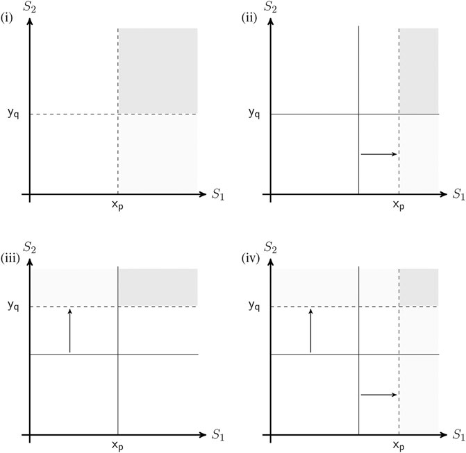
FIGURE 1. Exemplary quantile partitions and assessments of upper tail service time dependence.

It shows a sequence of assessing refined quantile partitions for a joint distribution’s upper tail via assessments of new quantile maxima from (ii) throughout (iv) following the initial assessment (i). This sequence refines a copula between service times exceeding certain thresholds. For instance in (i), we elicit the conditional probability of server S₂ exceeding its median given that server S₁ exceeds its median. This can be framed as follows:

“Given that S₁ exceeds its median value of x (minutes, hours, etc.), what is the probability that S₂ also exceeds its median value of y (minutes, hours, etc.)?”

In (ii) and (iii), we alternate between eliciting the probabilities of S₁ and S₂ exceeding some higher quantile, e.g. their 95th, given that the other service time is (still) above their median. Lastly, in (iv), we elicit the conditional probability of both S₁ and S₂ exceeding the higher quantile. In a similar way, we can elicit more quantile partitions and different quantiles. As such, in the illustrative case study we include the 75th and 95th quantiles together with the medians.

4.3 Implementing Minimum Information Copulas in DES Models

Once the minimum information copulas for the dependent service times are defined, we implement these in the DES model. By recording the unconditional service time (and corresponding quantile) at the first of two servers (e.g. S₁ in the above framing for Figure 1) for each serviced entity, we then sample that entity’s conditional service time at the other server (S₂ in the above example) from the minimum information copula as shown schematically in Figure 2 during run time of the simulation.

FIGURE 2

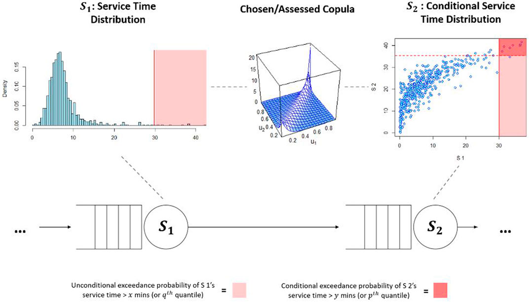
FIGURE 2. Schematic representation of conditional service time simulation from a copula.

We do this for every entity for which a conditional service time is sampled.

5 Illustrative Case Study: Impact of Tail Dependencies on an Emergency Ambulance Service Simulation

Decision-making in healthcare typically involves complex uncertainties which is why it often requires rigorous approaches to risk and decision analysis. Therefore, most public and private organisations in this sector rely on stochastic modelling of their systems and processes, such as simulation models, for making informed decisions. For overviews on DES applications in healthcare, see for instance Hamrock et al. [47], Jahangirian et al. [48], Gunal and Pidd [49] and Duguay and Chetouane [50].

An area of healthcare, in which complex uncertainties are of particular concern and where simulation can be an important basis for decision-making, is emergency ambulance service planning. Overviews on simulation studies for ambulance systems are provided by Pinto et al. [51] and Aboueljinane et al. [52]. Here, ensuring a patient’s timely aid and possibly transport to a hospital is critical. However, uncertainties around the durations of the different tasks involved in ambulance services pose a risk of underestimating the time needed for completing each emergency. This can mislead decision-makers involved in resource planning and dispatching of emergency units. This is especially critical whenever tail dependencies are of concern, potentially increasing the overall time per emergency drastically. This in turn might keep a higher number of ambulance units occupied for longer than expected. As such, questions regarding the availability of sufficient ambulance units (for particular types of emergencies) while still ensuring a high utilization due to economic reasons, need to be addressed by decision-makers and can benefit from more rigorous models.Therefore, we address the impact of tail dependencies on ambulance services in this illustrative case study. We will show a way of including risks from tail dependencies potentially affecting the maximum time in system for emergencies.

5.1 Background to Case Study: Simulation Set-Up and Dependence Assessments

The simulation in this illustrative case study has been developed together with an expert with over 4 years experience of working in an ambulance service in the United Kingdom. The expert’s practical experience, also considered as substantive expertise is what we are mostly after when selecting experts [53].

5.1.1 Simulated Ambulance Service Process

The focus of the simulation model presented here is on the journey of an ambulance (after being dispatched) and the tasks on scene at an emergency. The process ends once a patient has been transferred to a hospital and the unit is ready for the next emergency after some turn-around activities. This excludes and largely simplifies the call generation (demand side), i.e. modelling the frequency of incidents, and the dispatching of an ambulance service modelling part. In fact, we are only interested in simulating many single emergencies whereas a more complex model can be developed based on this by plugging in the inter-arrival times of emergency calls and running scenarios on the availability of multiple ambulance units and their utilization. Another assumption in this simulation is that there will always be a hospital accepting the emergency. In real systems, this might not always be the case which can increase the delay for transportation to a hospital significantly. We are focusing on ambulance performance measured by their maximum time in system for an emergency. The details of the simulated process are shown in Figure 3.

FIGURE 3

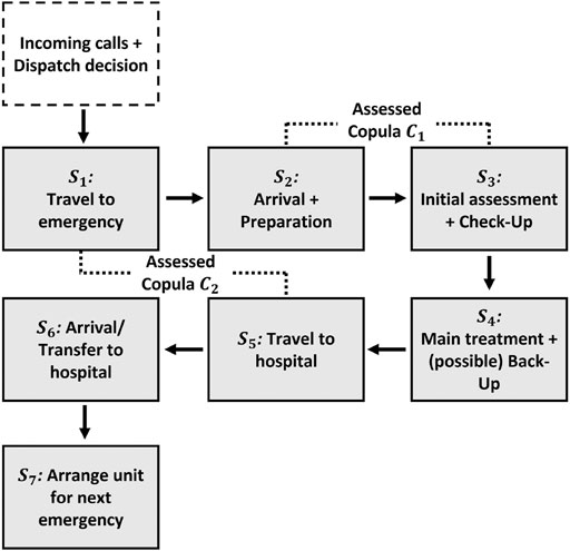
FIGURE 3. Simulated ambulance service process outline.

The different elements of the process, servers S₁ to S₇, and the corresponding univariate timing distributions for these were identified by our expert together with provided process maps and fitted from historical data (see Appendix for the details of the servers’ univariate distributions).

5.1.2 Identification and Assessment of Main Dependence Relationships

After having outlined and structured the various elements that are included in the simulated process, the same expert determined between which of these tasks there might be a potential (significant) impact due to dependencies. As shown in Figure 3, the probabilistic dependencies between “Travel to emergency” (S₁) and “Travel to hospital” (S₅) as well as between “Arrival and preparation” (S₂) and “Initial assessment” (S₃) are regarded to have a main impact (upper tail risk) for the maximum time in system measure to be significantly higher than in the same model assuming that all service times are independent.

Next, the expert assessed these dependence relationships quantitatively using the method presented in Section 4.2 and by that defined the minimum information copulas C₁ and C₂. C₁ is the copula of joint distribution $F_{S_1,S_5}$ and C₂ of $F_{S_2,S_3}$. Table 1 provides an overview of the assessments for C₂ together with the framing of the corresponding elicitation questions.

TABLE 1

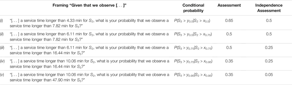
TABLE 1. Overview of dependence elicitation procedure and results for C₂.

In Table 1 we see that the expert considers there generally to be a positive dependence relationship between the service times of S₂ and S₃ as indicated by assessment (i), even if not a strong one (see Section 4.2 for an explanation on interpreting assessments). For (iii), the expert’s assessment is close to the resulting upper bound so that we can interpret it to indicate again positive dependence in the quadrant above both 75th quantiles, this time with high dependence strength. Similarly, for the extreme quadrant of S₂ and S₃ both being above their corresponding 95th quantiles the expert assesses there to be (strong) upper tail dependence. Note, we only elicited refinements on the upper right quadrant (above both medians) which results in less restrictive feasible bounds from the linear program and assumes that the probability mass in the remaining three quadrants (P(S₃ > y_0.5|S₂ ≤ x_0.5), P(S₃ ≤ y_0.5|S₂ > x_0.5), and P(S₃ ≤ y_0.5|S₂ ≤ x_0.5)) is equally distributed.

Table 2 (in the Appendix) shows the assessments for C₁. Here, we observe that while the expert assesses independence for the central distribution part, i.e. assessment (i), she then refines the upper tail in the following assessments (up to (v)) by assessing a positive dependence relationship in more extreme parts. However, overall she assesses less probability for the extreme quadrants than for the dependence between S₂ and S₃.

TABLE 2

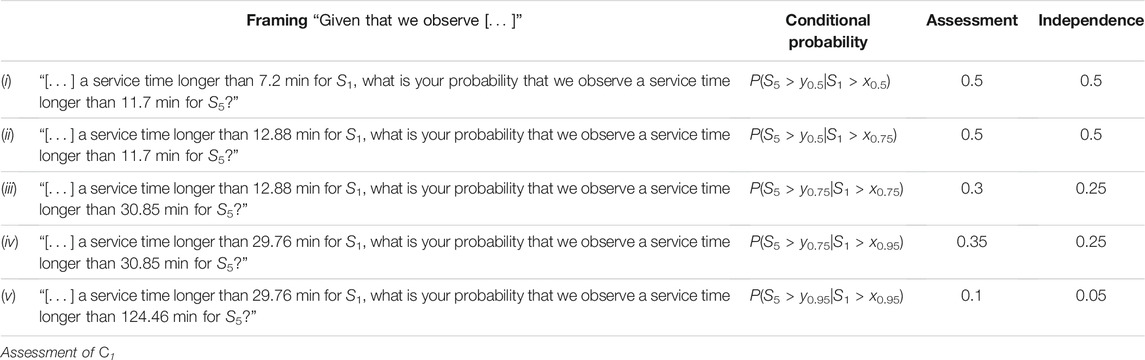
TABLE 2. Overview of dependence elicitation procedure and results for C₁.

The expert’s rationale for the assessments underlines that a potential tail dependence for C₂ stems from the initial situation at the emergency scene. In some emergencies, bystanders slow down the preparation (or set-up) of the unit, which includes unpacking necessary equipment as an essential part of S₂, while they also affect the first contact and initial assessment on the victim (S₃). An example is an emergency in which bystanders actively try to hinder the ambulance’s work, e.g. through harassment or interrupting otherwise. Another source of dependence between these tasks comes from the victim itself who might refuse treatment, again affecting both tasks similarly. While this might also affect S₄ as pointed out by the expert initially, in the final assessment she considered S₄ to be independent of S₂ and S₃, simply as the tasks in S₄ can be done quickly after S₃.

For C₁, the main source of potential tail dependence stems from the general traffic in the local area of the emergency occurring. That is, while the routes themselves from the base to the emergency and from there to the hospital are typically different, some external effects, such as a central road closure, can prolong both. Further, the time of the day, week etc. is likely to have an effect on both travel durations together. Due to such external events affecting any travel (within a certain local area), the expert assessed a likelihood of tail dependence between S₁ and S₅, i.e. C₁, even if not as strong as between the other two tasks (i.e. C₂).

5.1.3 Sensitivity of Tail Dependencies

Throughout this paper, we have used the term tail dependence so far in a general sense, referring to the situation of two extremely long service times, i.e. at two different servers, occurring for the same entity that is being serviced. However, as mentioned in Section 4.1.1, several tail dependence measures exist for analysing the upper and/or lower parts of a joint distribution more rigorously. In this context, we now look at our minimum information copulas and their tail dependence more closely. In particular, we want to better understand the impact of the joint distribution tails for when we simulate from our minimum information copula and by that their sensitivity with regards to the expert’s assessments on these.

To do so, we consider the assessed quadrants above the 50th, 75th, and 95th quantiles as the expert’s refined judgements on the upper tail and hence on the importance of tail dependence for the chosen service time relationships. In order to better understand the tail dependence of C₂, Figure 4 compares the different scatter-plots for the question of “what-if” the elicitation had stopped after assessment (i) and (iii) with (v) (in Table 1) accordingly. In other words, it considers the scenarios of only having refined the upper quadrants up to a certain level.

FIGURE 4

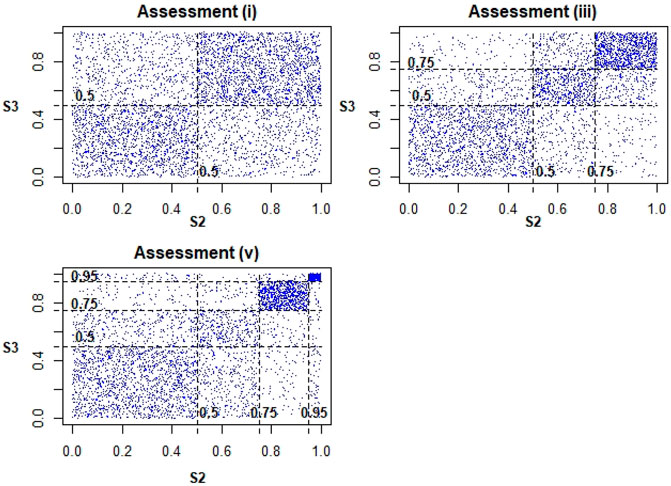
FIGURE 4. Resulting minimum information scatter-plots when stopping refinements after specific assessments for C₂.

It shows the impact that each refinement has on a more extreme quadrant with regards to the joint distribution’s upper tail. Similarly, Figure 5 shows how the estimated conditional probability P(S₃ > u|S₂ > u) differs for copulas (i), (iii), and (v) for different quantiles through the tail concentration function R(u) = P(S₃ > u|S₂ > u)/(1 − u)² [54].

FIGURE 5

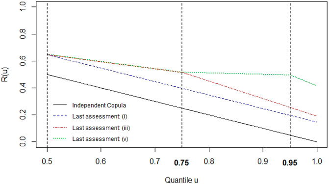
FIGURE 5. R(u) when stopping quadrant refinements after assessments (i), (iii), (v).

Following from that, we first measure the overall dependence strength of C₂ via Spearman’s rank correlation, ρ. Then, we use its conditional measure for the upper tail for each of the above versions of our minimum information copula ((i), (iii) and (v)) to obtain more insight on the difference in their tail dependence strength.

Spearman’s rank correlation is derived for a copula via (e.g. [42]):

$\rho (X,Y)=12{\iint }_{{[\mathrm{0,1}]}^2}C(u,v)\mathbf{d}u\mathbf{d}v-3(2)$

In order to obtain a rank correlation measure for the upper tail specifically, recall first that the copula of the conditional distribution P(U > x, V > y|U > u, V > v) on [u, 1] × [v, 1] is:

$\mathrm{\Phi }(C,u,v)(x,y)=\frac{C(1-F_X{(C,u,v)}^{-1}(x),1-F_Y{(C,u,v)}^{-1}(y))}{C(1-u,1-v)}(3)$

with $F_X(C,u,v)(x)=\frac{C(1-x,1-v)}{C(1-u,1-v)}$ and $F_Y(C,u,v)(y)=\frac{C(1-u,1-y)}{C(1-u,1-v)}$ accordingly. See Charpentier [55] for proofs and details. We can then derive a conditional rank correlation measure for the upper tail, on [u, 1] × [v, 1], (see [55] for details) through:

$\bar{\rho }(C,u,v)=12{\iint }_{{[\mathrm{0,1}]}^2}\mathrm{\Phi }(C,u,v)(x,y)\mathbf{d}x\mathbf{d}y-3(4)$

Using numerical integration, we then obtain an overall ρ of 0.372 and conditional tail measures are shown in Table 3.

TABLE 3

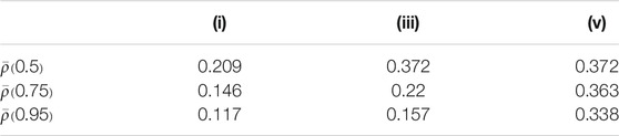
TABLE 3. Conditional correlation as Spearman’s rho (ρ) for the upper tail of C₂.

We can analyse the behaviour in the tails further if desired, in particular if we can assume that our minimum information copula is an extreme value (EV) distribution. P Capéraà and Genest [56] provide a non-parametric measure which has been frequently used for minimum information EV copulas.

However, from the above, we already observe that without further refinements after assessment (i), tail dependence decreases continuously and is low in the minimum information copula’s upper, extreme part. For the quadrant higher than the assessed 75th quantiles (i.e. with assessment (iii) included), the conditional $\bar{\rho }$ remains higher than before and decreases less. Lastly, with assessment (v) included, tail dependence remains at a high level the longest given the high probability assessment (proportionally to the provided upper bound) for the quadrant above both 95th quantiles.

5.1.4 Simulation of Ambulance Service

Finally, we built and ran the simulation in SIMUL8 [57]. We used its connection to spreadsheets and R [58], specifically the copula package [59], to first store the sampled service times of the unconditional tasks, i.e. at S₁ and S₂, and to then sample times for the conditional tasks using our minimum information copulas. Figure 6 shows the simulation together with annotations on where we stored the initial occurrences of exceeding a specific quantile in order to then sample the conditional service times.

FIGURE 6

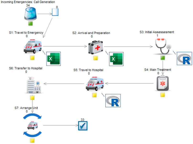
FIGURE 6. Simulation during run time (SIMUL8 screenshot with annotations).

5.2 Simulation Results and Discussion

With the dependence assessments and simulation model in place, we obtained the results to compare the different maximum times in system for the version of this simulation including the dependencies and another version assuming independence between all service times.

For both versions, we obtained the maximum times in system from 30 simulation runs for each of which the random number seeds¹ (for all distributions) were changed. In that way, we obtained 30 representative maximum time in system results for each version. Given that the simulation focuses on the process of single emergencies, note within each simulation run we simulated >50 emergencies. Each simulation version’s maximum time in system results are summarized in the box-plots in Figure 7.

FIGURE 7

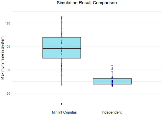
FIGURE 7. Comparison of maximum times in system (in minutes) for simulation with dependent and independent service times.

We observe that both simulation versions perform quite differently regarding the generated maximum time in system results. As such, the median of the simulation version with independent service times (70.37 min) is lower than even the 25th quartile of the box-plot for the simulation version including the assessed minimum information copulas which is 89.92 min. In fact, this median result would fall within the extreme results on the other simulation’s lower end. The inter-quartile ranges are not overlapping and the box-plot resulting from the simulation version assuming independence between service times (25th: 67.73, 50th: 70.37, 75th: 72.49 min) is much narrower compared to the other version (25th: 89.92, 50th: 98.22, 75th: 107.87 min). This shows an overall higher uncertainty around this result for when we include the assessed dependencies. In particular the number of extreme simulation results above the corresponding 75th and 95th quartiles are of interest. It shows the impact that exceeding a certain service time quantile for either S₁ or S₂ can have by likely triggering higher service times in the corresponding conditional tasks, possibly resulting in (much) higher maximum time in system results. Thus, even in such a simple process, the upper tail risk of our assessed copulas can have a significant impact.

5.3 Reflections on Illustrative Case Study

While more research and insight on simulation problems with potentially dependent service times is needed to better understand how (tail) dependence risk can propagate to simulation results, we consider the proposed method to be suitable for improving its understanding in our context and by that informing decision-making in emergency ambulance service planning. Even in this small case study, we already see that the impact of tail dependencies can be considerable for the overall time an ambulance unit spends on an emergency and hence is ready to be deployed again. This can have a significant impact on planning unit availability and other aspects of resource scheduling and staffing.

Nevertheless, the complexity of the simulation in our illustrative case study is limited and only included one expert. In future, it will be important to test the proposed method for more complex ambulance service simulations. In particular, it will be interesting to weight in the benefits of assessing more possible dependencies in a simulation against the challenges of dealing with experts’ increased cognitive challenges to do so. There is a balance between assessing the relationships between all service times, which is most likely not possible with regards to time and willingness of experts to make that many assessments, and assessing too few dependencies, thereby possibly omitting or underestimating important ones. For the small simulation in this case study the expert was comfortable with identifying the most critical dependencies before assessing them. However, this cannot always be assumed. For instance, Anagnostou and Taylor [60] outline that ambulance service simulations should include the Accident and Emergency (A&E) department, as they are interwoven with the emergency medical services. This would already increase the complexity of the above model significantly. Therefore, in future case studies on DES models with dependencies, we should integrate methods for structuring experts’ knowledge to first judge which and hence how many dependence relationships to include and asses. In that way, omissions of dependencies are more structured and justifiable than in the previous case study.

Lastly, including more experts that work on the different aspects of ambulance services might improve the robustness of the assessed dependencies. Therefore, future applications should include multiple, different experts on ambulance services and their additional insight should be evaluated.

6 Conclusions and Future Research

In this paper, we have introduced a method for including potential tail dependencies between service time distributions as these can significantly impact important simulation results, commonly sought after in DES, whenever we cannot assume independence. Especially, we considered the simulation result of maximum time in system in this context. We have shown in the illustrative case study that for ambulance services the maximum time in system is critical whereas it can be impacted by possible tail dependencies.

While this paper gives the reader a general introduction to including tail dependencies in DES and answers questions about why a modeller might do so by outlining their sources, the main contribution is the LP-based expert judgement method presented. It offers flexibility in terms of assessing copulas to a level as desired by a decision-maker and addressing the modelling challenge of lacking historical data on dependencies between service times. We regard it as an important tool for any modeller whenever facing this modelling challenge in order to ensure robust simulation results and hence robust decisions based on these in the face of tail dependence risks. Already Robinson [1] points out that simulation models are “data hungry”. Therefore, offering structured ways of assessing missing data can be even of broader interest for the simulation community, not only in the context of tail dependencies.

In future research, it is desirable to consider tail dependencies for more complex simulations and by that explore how comfortable experts are with assessing minimum information copulas for other simulation problems. An example is developing a DES for a non-existing system or process, such as a new factory design or a newly proposed clinical pathway for patients. Here, dependencies and their assessments might be more debatable among the experts and decision-makers. In this regard, the number of assessments to make in order to obtain sufficiently detailed minimum information copulas might be addressed given that the proposed method offers flexibility on that. Further, in future research we should explore experts’ willingness and ability to assess dependence relationships in higher dimensions as these might be important to consider for many simulation problems. For these, we elicit conditional probabilities with a conditioning set of more than one condition whereas the question can be framed e.g. as “Given that not only S₁ but also S₂ exceed their median values of $x_{S_1}$ and $x_{S_2}$ minutes, what is the probability that S₃ exceeds its median value of y minutes?”. While our method provides feasible upper and lower bounds for such assessments and a minimum information copula in higher dimensions, it is important to consider experts’ potential cognitive challenges when making such assessments.

Next, including more experts and ones from different backgrounds will be important in future dependence assessments on DES models as they offer a wider perspective on the uncertainties involved. In DES, we often require experts on the whole simulated process, but also ones for specific sub-parts, such as clinicians making decisions in one specific part while nurses are involved in other process steps. With multiple experts, we then also need to explore sensible ways of combining dependence assessments which is currently a little explored research area [61].

Lastly, when reflecting on our case study in the previous section, we already highlighted the importance of more structured ways to support experts’ in the initial decision on which dependencies to include.

Quantile Partition and LP Example for Feasible Assessment Bounds

Based on the earlier example of a common assessment sequence as shown in Figure 1, we present the corresponding quantile partition together with the LP problem for obtaining assessments’ feasible bounds. Figure 8 shows the resulting quantile partition.

FIGURE 8

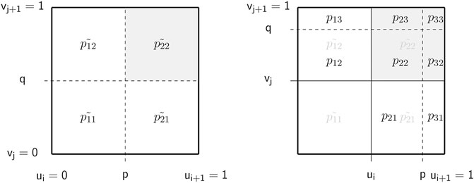
FIGURE 8. Quantile partition of the joint distribution from (i) to (iv).

Based on Figure 8, we can now formulate the following LP problem to determine the feasible bounds:

$\left.\begin{array}{c}\hfill \min ,\hfill \\ \hfill \max \hfill \end{array}\right\}{p}_{33}(5)$

subject to

$\begin{array}{c}\hfill p_{13}+p_{12}=\widetilde{p_{12}}\hfill \\ \hfill p_{23}+p_{22}+p_{33}+p_{32}=\widetilde{p_{22}}\hfill \\ \hfill p_{11}=\widetilde{p_{11}}\hfill \end{array}$

and

$\begin{array}{c}\hfill p_{21}+p_{31}=\widetilde{p_{12}}\hfill \end{array}$

Data Availability Statement

The raw data supporting the conclusion of this article will be made available by the authors, without undue reservation.

Author Contributions

CW conducted the dependence elicitation and constructed the DES model. Further, CW wrote the complete manuscript.

Author Disclaimer

The findings in this paper express the author’s own views.

Conflict of Interest

Author CW is employed by company Simul8. The company was not involved in the study design, collection, analysis, interpretation of data, the writing of this article or the decision to submit it for publication.

Publisher’s Note

All claims expressed in this article are solely those of the authors and do not necessarily represent those of their affiliated organizations, or those of the publisher, the editors and the reviewers. Any product that may be evaluated in this article, or claim that may be made by its manufacturer, is not guaranteed or endorsed by the publisher.

Footnotes

¹In SIMUL8 and simulation generally, we include randomness via streams of pseudo-random numbers which create a simulation’s random events and timings according to the defined statistical patterns.

References

1. Robinson, S. Simulation: The Practice of Model Development and Use. Hampshire: Palgrave MacMillan (2014).

Google Scholar

2. Robinson, S. Conceptual Modelling for Simulation Part I: Definition and Requirements. J Oper Res Soc (2008) 59:278–90. doi:10.1057/palgrave.jors.2602368

CrossRef Full Text | Google Scholar

3. Taylor, S, Chick, S, Macal, C, Brailsford, S, L’Ecuyer, P, and Nelson, B. Modeling and Simulation Grand Challenges: An Or/ms Perspective. In: Proceedings of the 2013 Winter Simulation Conference (INFORMS); 8-11 Dec. 2013; Washington, DC, USA. IEEE (2013) p. 1269–82. doi:10.1109/wsc.2013.6721514

CrossRef Full Text | Google Scholar

4. Cheng, R. History of Input Modeling. In: Proceedings of the 2017 Winter Simulation Conference (INFORMS); 3-6 Dec. 2017; Las Vegas, NV, USA. IEEE (2017) p. 181–201. doi:10.1109/wsc.2017.8247789

CrossRef Full Text | Google Scholar

5. Biller, B, and Ghosh, S. Chapter 5 Multivariate Input Processes. Handbooks Operations Res Manag Sci (2006) 13:123–53. doi:10.1016/s0927-0507(06)13005-4

CrossRef Full Text | Google Scholar

6. Pasupathy, R, and Nagaraj, K. Modeling Dependence in Simulation Input: The Case for Copulas. In: Proceedings of the 2015 Winter Simulation Conference (INFORMS); 6-9 Dec. 2015; Huntington Beach, CA, USA. IEEE (2015) p. 1850–64. doi:10.1109/wsc.2015.7408300

CrossRef Full Text | Google Scholar

7. Biller, B. Copula-based Multivariate Input Models for Stochastic Simulation. Operations Res (2009) 57:878–92. doi:10.1287/opre.1080.0669

CrossRef Full Text | Google Scholar

8. Biller, B, and Gunes Corlu, C. Copula-based Multivariate Input Modeling. Surv Operations Res Manag Sci (2012) 17:69–84. doi:10.1016/j.sorms.2012.04.001

CrossRef Full Text | Google Scholar

9. Mitchell, CR, Paulson, AS, and Beswick, CA. The Effect of Correlated Exponential Service Times on Single Server Tandem Queues. Naval Res Logistics (1977) 24:95–112. doi:10.1002/nav.3800240108

CrossRef Full Text | Google Scholar

10. Pinedo, M, and Wolff, RW. A Comparison between Tandem Queues with Dependent and Independent Service Times. Operations Res (1982) 30:464–79. doi:10.1287/opre.30.3.464

CrossRef Full Text | Google Scholar

11. Wilson, J. Modeling Dependencies in Stochastic Simulation Inputs. In: Proceedings of the 1997 Winter Simulation Conference (INFORMS); December 7-10, 1997; Atlanta Georgia USA. IEEE (1997) p. 47–52. doi:10.1145/268437.268446

CrossRef Full Text | Google Scholar

12. Ibrahim, R, Ye, H, L’Ecuyer, P, and Shen, H. Modeling and Forecasting Call center Arrivals: A Literature Survey and a Case Study. Int J Forecast (2016) 32:865–74. doi:10.1016/j.ijforecast.2015.11.012

CrossRef Full Text | Google Scholar

13. Biller, B, and Corlu, CG. Accounting for Parameter Uncertainty in Large-Scale Stochastic Simulations with Correlated Inputs. Operations Res (2011) 59:661–73. doi:10.1287/opre.1110.0915

CrossRef Full Text | Google Scholar

14. Channouf, N, and L'Ecuyer, P. A normal Copula Model for the Arrival Process in a Call center. Intl Trans Op Res (2012) 19:771–87. doi:10.1111/j.1475-3995.2012.00845.x

CrossRef Full Text | Google Scholar

15. Bedford, T, and Cooke, R. Vines-a New Graphical Model for Dependent Random Variables. Ann Stat (2002) 30:1031–68. doi:10.1214/aos/1031689016

CrossRef Full Text | Google Scholar

16. Gans, N, Liu, N, Mandelbaum, A, Shen, H, and Ye, H. Service Times in Call Centers: Agent Heterogeneity and Learning with Some Operational Consequences. In: J Berger, T Cai, and I Johnstone, editors. Borrowing Strength: Theory Powering Applications - A Festschrift for Lawrence D. Brown. Beachwood: Institute for Mathematical Statistics (2010) p. 99–123. doi:10.1214/10-imscoll608

CrossRef Full Text | Google Scholar

17. Dong, J, Feldman, P, and Yom-Tov, GB. Service Systems with Slowdowns: Potential Failures and Proposed Solutions. Operations Res (2015) 63:305–24. doi:10.1287/opre.2015.1346

CrossRef Full Text | Google Scholar

18. Chan, CW, Yom-Tov, G, and Escobar, G. When to Use Speedup: An Examination of Service Systems with Returns. Operations Res (2014) 62:462–82. doi:10.1287/opre.2014.1258

CrossRef Full Text | Google Scholar

19. Brown, L, Gans, N, Mandelbaum, A, Sakov, A, Shen, H, Zeltyn, S, et al. Statistical Analysis of a Telephone Call Center. J Am Stat Assoc (2005) 100:36–50. doi:10.1198/016214504000001808

CrossRef Full Text | Google Scholar

20. Armony, M. Dynamic Routing in Large-Scale Service Systems with Heterogeneous Servers. Queueing Syst (2005) 51:287–329. doi:10.1007/s11134-005-3760-7

CrossRef Full Text | Google Scholar

21. Armony, M, and Mandelbaum, A. Routing and Staffing in Large-Scale Service Systems: The Case of Homogeneous Impatient Customers and Heterogeneous Servers. Operations Res (2011) 59:50–65. doi:10.1287/opre.1100.0878

CrossRef Full Text | Google Scholar

22. Gans, N, Koole, G, and Mandelbaum, A. Telephone Call Centers: Tutorial, Review, and Research Prospects. M&SOM (2003) 5:79–141. doi:10.1287/msom.5.2.79.16071

CrossRef Full Text | Google Scholar

23. Xie, W, Li, C, and Zhang, P. A Factor-Based Bayesian Framework for Risk Analysis in Stochastic Simulations. ACM Trans Model Comput Simul (2017) 27:1–31. doi:10.1145/3154387

CrossRef Full Text | Google Scholar

24. Pang, G, and Whitt, W. The Impact of Dependent Service Times on Large-Scale Service Systems. M&SOM (2012) 14:262–78. doi:10.1287/msom.1110.0363

CrossRef Full Text | Google Scholar

25. L’Ecuyer, P, Gustavsson, K, and Olsson, L. Modeling Bursts in the Arrival Process to an Emergency Call center. In: Proceesings of the 2018 Winter Simulation Conference; 9-12 Dec. 2018; Gothenburg, Sweden. IEEE (2018) p. 525–36. doi:10.1109/WSC.2018.8632536

CrossRef Full Text | Google Scholar

26. Brailsford, SC, Eldabi, T, Kunc, M, Mustafee, N, and Osorio, AF. Hybrid Simulation Modelling in Operational Research: A State-Of-The-Art Review. Eur J Oper Res (2019) 278:721–37. doi:10.1016/j.ejor.2018.10.025

CrossRef Full Text | Google Scholar

27. Stanfield, PM, Wilson, JR, and King, RE. Flexible Modelling of Correlated Operation Times with Application in Product-Reuse Facilities. Int J Prod Res (2004) 42:2179–96. doi:10.1080/0020754042000203903

CrossRef Full Text | Google Scholar

28. Jaoua, A, L’Ecuyer, P, and Delorme, L. Call-type Dependence in Multiskill Call Centers. Simulation (2013) 89:722–34. doi:10.1177/0037549713479405

CrossRef Full Text | Google Scholar

29. Biller, B, and Gunes, C. Introduction to Simulation Input Modeling. In: Proceedings of the 2010 Winter Simulation Conference; 5-8 Dec. 2010; Baltimore, MD, USA. IEEE (2010) p. 49–58. doi:10.1109/wsc.2010.5679176

CrossRef Full Text | Google Scholar

30. Corlu, C, Akcay, A, and Xie, W. Stochastic Simulation under Input Uncertainty: A Review. Operations Res Perspect (2020) 7:100–62. doi:10.1016/j.orp.2020.100162

CrossRef Full Text | Google Scholar

31. Wagner, MAF, and Wilson, JR. Graphical Interactive Simulation Input Modeling with Bivariate Bézier Distributions. ACM Trans Model Comput Simul (1995) 5:163–89. doi:10.1145/217853.217854

CrossRef Full Text | Google Scholar

32. Ghosh, S, and Henderson, SG. Patchwork Distributions. In: C Alexopoulos, D Goldsman, and J Wilson, editors. Advancing the Frontiers of Simulation: A Festschrift in Honor of George S. Fishman. Cham: Springer (2009) p. 65–86. doi:10.1007/b110059_4

CrossRef Full Text | Google Scholar

33. Clemen, RT, Fischer, GW, and Winkler, RL. Assessing Dependence: Some Experimental Results. Manag Sci (2000) 46:1100–15. doi:10.1287/mnsc.46.8.1100.12023

CrossRef Full Text | Google Scholar

34. Werner, C, Bedford, T, Cooke, RM, Hanea, AM, and Morales-Nápoles, O. Expert Judgement for Dependence in Probabilistic Modelling: a Systematic Literature Review and Future Research Directions. Eur J Oper Res (2017) 258:801–19. doi:10.1016/j.ejor.2016.10.018

CrossRef Full Text | Google Scholar

35. Werner, C, Bedford, T, and Quigley, J. Sequential Refined Partitioning for Probabilistic Dependence Assessment. Risk Anal (2018) 38:2683–702. doi:10.1111/risa.13162

PubMed Abstract | CrossRef Full Text | Google Scholar

36. Werner, C, Bedford, T, and Quigley, J. Mapping Conditional Scenarios for Knowledge Structuring in (Tail) Dependence Elicitation. J Oper Res Soc (2020) 72:889–907. doi:10.1080/01605682.2019.1700767

CrossRef Full Text | Google Scholar

37. Bedford, T, Daneshkhah, A, and Wilson, KJ. Approximate Uncertainty Modeling in Risk Analysis with Vine Copulas. Risk Anal (2016) 36:792–815. doi:10.1111/risa.12471

PubMed Abstract | CrossRef Full Text | Google Scholar

38. Kotz, S, and van Dorp, JR. Generalized diagonal Band Copulas with Two-Sided Generating Densities. Decis Anal (2010) 7:196–214. doi:10.1287/deca.1090.0162

CrossRef Full Text | Google Scholar

39. Al-Awadhi, SA, and Garthwaite, PH. Prior Distribution Assessment for a Multivariate normal Distribution: an Experimental Study. J Appl Stat (2001) 28:5–23. doi:10.1080/02664760120011563

CrossRef Full Text | Google Scholar

40. Dickey, JM, Lindley, DV, and Press, SJ. Bayesian Estimation of the Dispersion Matrix of a Multivariate normal Distribution. Commun Stat - Theor Methods (1985) 14:1019–34. doi:10.1080/03610928508828960

CrossRef Full Text | Google Scholar

41. Joe, H. Dependence Modeling with Copulas. New York: CRC Press (2014).

Google Scholar

42. Nelsen, R. An Introduction to Copulas. New York: Springer Science and Business Media (2007).

Google Scholar

43. Embrechts, P, McNeil, AJ, and Straumann, D. Correlation and Dependence in Risk Management: Properties and Pitfalls. Risk Manag value Risk beyond (2002) 1:176–223. doi:10.1017/cbo9780511615337.008

CrossRef Full Text | Google Scholar

44. Meeuwissen, AMH, and Bedford, T. Minimally Informative Distributions with Given Rank Correlation for Use in Uncertainty Analysis. J Stat Comput Simulation (1997) 57:143–74. doi:10.1080/00949659708811806

CrossRef Full Text | Google Scholar

45. Bedford, T, and Wilson, KJ. On the Construction of Minimum Information Bivariate Copula Families. Ann Inst Stat Math (2014) 66:703–23. doi:10.1007/s10463-013-0422-0

CrossRef Full Text | Google Scholar

46. Kullback, S, and Leibler, RA. On Information and Sufficiency. Ann Math Statist (1951) 22:79–86. doi:10.1214/aoms/1177729694

CrossRef Full Text | Google Scholar

47. Hamrock, E, Paige, K, Parks, J, Scheulen, J, and Levin, S. Discrete Event Simulation for Healthcare Organizations: a Tool for Decision Making. J Healthc Manag (2013) 58:110–24. doi:10.1097/00115514-201303000-00007

CrossRef Full Text | Google Scholar

48. Jahangirian, M, Naseer, A, Stergioulas, L, Young, T, Eldabi, T, Brailsford, S, et al. Simulation in Health-Care: Lessons from Other Sectors. Oper Res Int J (2012) 12:45–55. doi:10.1007/s12351-010-0089-8

CrossRef Full Text | Google Scholar

49. Günal, MM, and Pidd, M. Discrete Event Simulation for Performance Modelling in Health Care: a Review of the Literature. J Simulation (2010) 4:42–51. doi:10.1057/jos.2009.25

CrossRef Full Text | Google Scholar

50. Duguay, C, and Chetouane, F. Modeling and Improving Emergency Department Systems Using Discrete Event Simulation. Simulation (2007) 83:311–20. doi:10.1177/0037549707083111

CrossRef Full Text | Google Scholar

51. Pinto, LR, Silva, PMS, and Young, TP. A Generic Method to Develop Simulation Models for Ambulance Systems. Simulation Model Pract Theor (2015) 51:170–83. doi:10.1016/j.simpat.2014.12.001

CrossRef Full Text | Google Scholar

52. Aboueljinane, L, Sahin, E, Jemai, Z, and Marty, J. A Simulation Study to Improve the Performance of an Emergency Medical Service: Application to the French Val-De-marne Department. Simulation Model Pract Theor (2014) 47:46–59. doi:10.1016/j.simpat.2014.05.007

CrossRef Full Text | Google Scholar

53. Bolger, F. The Selection of Experts for (Probabilistic) Expert Knowledge Elicitation. In: L Dias, A Morton, and J Quigley, editors. Elicitation. Cham: Springer (2018) p. 393–443. doi:10.1007/978-3-319-65052-4_16

CrossRef Full Text | Google Scholar

54. Venter, G. Tails of Copulas. Proc Casualty Actuarial Soc (2002) 89:68–113.

Google Scholar

55. Charpentier, A. Tail Distribution and Dependence Measures. Proc 34th ASTIN Conf (2003) 171, 1–25.

Google Scholar

56. Caperaa, P, and Genest, C. A Nonparametric Estimation Procedure for Bivariate Extreme Value Copulas. Biometrika (1997) 84:567–77. doi:10.1093/biomet/84.3.567

CrossRef Full Text | Google Scholar

57.SIMUL8. Simul8 Software (2020). Available from: www.Simul8.com (Accessed November 7, 2020).

Google Scholar

58.R Core Team. R. A Language and Environment for Statistical Computing. Vienna, Austria: R Foundation for Statistical Computing (2020).

Google Scholar

59. Hofert, M, Kojadinovic, I, Maechler, M, and Yan, J. Copula: Multivariate Dependence with Copulas (2020) R Package Version 1.0-1.

Google Scholar

60. Anagnostou, A, and Taylor, SJE. A Distributed Simulation Methodological Framework for Or/ms Applications. Simulation Model Pract Theor (2017) 70:101–19. doi:10.1016/j.simpat.2016.10.007

CrossRef Full Text | Google Scholar

61. Werner, C, Hanea, AM, and Morales-Nápoles, O. Eliciting Multivariate Uncertainty from Experts: Considerations and Approaches along the Expert Judgement Process. In: L Dias, A Morton, and J Quigley, editors. Elicitation. Cham: Springer (2018) 171–210. doi:10.1007/978-3-319-65052-4_8

CrossRef Full Text | Google Scholar

Appendix

Marginal Service Time Distributions (In Minutes):

$S_1\sim \mathsf{L}\mathsf{o}\mathsf{g}\mathsf{n}\mathsf{o}\mathsf{r}\mathsf{m}\mathsf{a}\mathsf{l}(7.2,2.37)$

$S_2\sim \mathsf{L}\mathsf{o}\mathsf{g}\mathsf{n}\mathsf{o}\mathsf{r}\mathsf{m}\mathsf{a}\mathsf{l}(4.33,1.67)$

$S_3\sim \mathsf{L}\mathsf{o}\mathsf{g}\mathsf{n}\mathsf{o}\mathsf{r}\mathsf{m}\mathsf{a}\mathsf{l}(7.82,3.01)$

$S_4\sim \mathsf{E}\mathsf{r}\mathsf{l}\mathsf{a}\mathsf{n}\mathsf{g}(11.6,8.35)$

$S_5\sim \mathsf{L}\mathsf{o}\mathsf{g}\mathsf{n}\mathsf{o}\mathsf{r}\mathsf{m}\mathsf{a}\mathsf{l}(11.7,4.21)$

$S_6\sim \mathsf{G}\mathsf{a}\mathsf{m}\mathsf{m}\mathsf{a}(6.89,0.65)$

$S_7\sim \mathsf{G}\mathsf{a}\mathsf{m}\mathsf{m}\mathsf{a}(8.46,0.27)$