Calibrating and Simulating Copula Functions in Financial Applications

Introduction

The study of the copula functions is very relevant because of their implementation in the field of financial portfolio risk management. The copula functions are used in financial applications since 2000, following the seminal researches of [1, 2]. The crucial matter is the real distribution of financial data. Empirical evidence has widely proved that the multinormal distribution is inadequate to model portfolio’s financial asset returns distribution at least from two points of view:

(1) The empirical marginal distributions are skewed and fat-tailed.

(2) The normal distribution does not consider the possibility of extreme joint co-movements for financial asset returns.

In other words, the real dependence structure of the financial assets is different from the Gaussian one and especially under situations of market stress [3]. For this reason, the copula functions can be a useful and simple tool for implementing efficient algorithms and to simulate the financial asset returns distribution more realistically.

The copulas allow us to model the dependence structure independently from the marginal distributions. In this way, we may construct a multivariate distribution with different margins and the dependence structure given from a particular type of copula function. Therefore, a crucial step in this context is the choice and the calibration of the most adequate copula function from the real financial data.

In this paper, a group of useful methods for calibrating, selecting, and simulating copula functions is presented. We aim to collect and to describe in a very simple manner the principal contributions in this field provided by the most famous and accredited international literature (for example [4–18]). In our opinion, the study of copula functions is very important because these quantitative tools are valuable for developing advanced financial portfolio models. Potential applications are in the field of market, credit, and operational risks. In particular, the copula functions can model the dependence structure between risk factors (for example, equity returns, interest rate returns, and foreign exchange returns) in a more reliable way.

In particular, the credit assets clearly show a non-normal return distribution and the phenomena of asymmetry, leptokurtosis, and tail dependence. To take into account these empirical characteristics of credit asset return distributions, with particular regard to multiple default events, we may model the default dependence structure by using different types of copulas. Technically, the times until default of each obligor in the loan portfolio may be simulated following a copula-based approach first illustrated in Li [1].

The copula functions have been also applied in the field of portfolio credit asset allocation where the optimal portfolio composition [19] may change by utilizing various types of the copula. The crucial aspect is the choice of the kind of copula better describing the default dependence structure of credit assets in a portfolio (see, for example [20]).

Further applications of copula functions in the financial risk management have been also developed by [21–25]. Nowadays, the copula functions find a precious application also in the estimate of the systemic risk generated by the Systemically Important Financial Institutions (see, for example [26–28]).

The implications in the field of the macro-prudential regulation on the global financial system are evident [29, 30].

Finally, in this paper, the described statistical methods for calibrating, selecting, and simulating copula functions are implemented to an empirical financial data set concerning the log-returns of two Italian equities: Olivetti and TIM. When it is possible, we show as the copula approach performs better than the bivariate normal distribution in modeling the real financial data.

The paper is structured as follows. In Definition of the Copula Function Section, a brief definition of copula function is given, describing the main families of copulas utilized in financial practical applications¹. In Parameter Estimation of a Given Copula Section, some quantitative approaches to estimate the parameters of a determined copula function from real data are presented. The procedures for selecting the type of copula function which better fits empirical data are shown in Selecting the Right Copula Section. In Simulation Algorithms Section, the algorithms to simulate random variates from some types of copula are illustrated. An application to a time series of the log-returns for two Italian equities is performed in Application to Two Italian Equities Section. Finally, in Concluding Remarks section, we draw some concluding remarks.

Definition of the Copula Function

An n-dimensional copula² is a multivariate distribution function (d.f.) C, with uniform distributed margins in [0, 1] (U(0, 1)) and the following properties:

1. C: [0, 1]ⁿ → [0, 1];

2. C is grounded and n-increasing;

3. C has margins C_i which satisfy C_i(u) = C(1, … , 1, u, 1, … , 1) = u for all u ∈ [0, 1].

It is obvious, from the above definition, that if F₁, … , F_n are univariate distribution functions, C(F₁(x₁), … , F_n(x_n)) is a multivariate d.f. with margins F₁, …, F_n, because U_i = F_i(X_i), i = 1, … , n, is a uniform random variable. Copula functions are a useful tool to construct and simulate multivariate distributions.

The following theorem is known as Sklar’s Theorem [31, 32]. It is the most important theorem about copula functions because it is used in many practical applications.

Theorem³: Let F be an n-dimensional d.f. with continuous margins F₁,…, F_n. Then it has the following unique copula representation:

$F(x_1,\dots ,x_n)=C(F_1\left(x_1\right),\dots ,F_n\left(x_n\right)).(1)$

From Sklar’s Theorem we see that, for continuous multivariate distribution functions, the univariate margins and the multivariate dependence structure can be separated. The dependence structure can be represented by a proper copula function. Moreover, the following corollary is attained from (1).

Corollary: Let F be an n-dimensional d.f. with continous margins F₁,…, F_nand copula C (satisfying(1)). Then, for anyu = (u₁,…, u_n) in [0, 1]ⁿ:

$C(u_1,\dots ,u_n)=F\left(F_1^{-1}\left(u_1\right),\dots ,F_n^{-1}\left(u_n\right)\right),(2)$

where F_i⁻¹is the generalized inverse of F_i.

A trivial example is the copula of independent random variables (the product copula). It takes the following form:

$C_{ind}(u_1,\dots ,u_n)=u_1\cdot \dots \cdot u_n.$

Another example is the Farlie–Gumbel–Morgenstern (FGM) copula, which in the bivariate case is defined by:

$C(u_1,u_2)=u_1{u}_2\left[1+\alpha (1-u_1)(1-u_2)\right],-1\le \alpha \le 1.$

Elliptical Copulas

The class of elliptical distributions provides useful examples of multivariate distributions because they share many of the tractable properties of the multivariate normal distribution. Furthermore, they allow modeling multivariate extreme events and forms of non-normal dependencies. Elliptical copulas are simply the copulas of elliptical distributions. Simulation from elliptical distributions is easy to perform. Therefore, as a consequence of Sklar’s Theorem⁴, the simulation of elliptical copulas is also easy.

Normal Copula

The Gaussian (or normal) copula is the copula of the multivariate normal distribution. The random vector X = (X₁, …, X_n) is multivariate normal iff:

(1) The univariate margins F₁, …, F_n are Gaussians;

(2) The dependence structure among the margins is described by a unique copula function C (the normal copula) such that⁵:

$C_R^{Ga}(u_1,\dots ,u_n)={\Phi }_R\left({\phi }^{-1}\left(u_1\right),\dots ,{\phi }^{-1}\left(u_n\right)\right),(3)$

where ${\Phi }_R$ is the standard multivariate normal d.f. with linear correlation matrix R and ${\phi }^{-1}$ is the inverse of the standard univariate Gaussian d.f.

If n = 2, Eq. 3 can be written as:

$C_R^{Ga}(u,v)={\displaystyle \underset{-\infty }{\overset{{\phi }^{-1}\left(u\right)}{\int }}{\displaystyle \underset{-\infty }{\overset{{\phi }^{-1}\left(v\right)}{\int }}\frac{1}{2\pi {(1-R_{12}^2)}^{1/2}}\exp \left\{-\frac{s^2-2R_{12}st+t^2}{2(1-R_{12}^2)}\right\}\text{d}s\text{d}t}},$

where R₁₂ is simply the linear correlation coefficient between the two random variables.

t-Student Copula

The copula of the multivariate t-Student distribution is the t-Student copula. Let X be a vector with an n-variate t-Student distribution with $\nu$ degrees of freedom, mean vector $\mathbf{\mu }$ (for $\nu >1$), and covariance matrix $\frac{\nu }{\nu -2}\Sigma$ (for $\nu >2$)⁶. It can be represented in the following way:

$\mathbf{X}\stackrel{\mathbf{d}}{=}\mathbf{\mu }+\frac{\sqrt{\nu }}{\sqrt{S}}\mathbf{Z},(4)$

where $\mathbf{\mu }\in R^n$S∼${\chi }_{\nu }^2$ and the random vector Z∼$N_n(\mathbf{0},\Sigma )$ are independent.

The copula of vector X is the t-Student copula with $\upsilon$ degrees of freedom. It can be analytically represented in the following way:

$C_{\nu ,R}^t\left(\mathbf{u}\right)=t_{\nu ,R}^n\left(t_{\nu }^{-1}\left(u_1\right),\dots ,t_{\nu }^{-1}\left(u_n\right)\right),(5)$

where $R_{ij}={\Sigma }_{ij}/\sqrt{{\Sigma }_{ii}{\Sigma }_{jj}}$ for $i,j\in \left\{1,\dots ,n\right\}$ and where $t_{\nu ,R}^n$ denotes the multivariate d.f. of the random vector $\sqrt{\nu }\mathbf{Y}/\sqrt{S}$, where the random variable S∼${\chi }_{\nu }^2$ and the random vector Y⁷ are independent. $t_{\nu }$ denotes the margins⁸ of $t_{\nu ,R}^n$.

For n = 2, the t-Student copula has the following analytic form:

$C_{\nu ,R}^t(u,v)={\displaystyle {\int }_{-\infty }^{t_{\nu }^{-1}\left(u\right)}{\displaystyle {\int }_{-\infty }^{t_{\nu }^{-1}\left(v\right)}\frac{1}{2\pi {(1-R_{12}^2)}^{1/2}}{\left\{1+\frac{s^2-2R_{12}st+t^2}{\nu (1-R_{12}^2)}\right\}}^{-(\nu +2)/2}\text{d}s\text{d}t}},$

where R₁₂ is the linear correlation coefficient of the bivariate t-Student distribution with $\nu$ degrees of freedom, if $\nu >2$.

Archimedean Copulas

An Archimedean copula can be written in the following form:

$C(u_1,\dots ,u_n)={\psi }^{-1}\left[\psi \left(u_1\right)+\cdots +\psi \left(u_n\right)\right](6)$

for all $0\le u_1,\dots ,u_n\le 1$ and where $\psi$ is a function often called the generator, satisfying:

i. $\psi \left(1\right)=0$;

ii. for all $t\in \left(\mathrm{0,1}\right),{\psi }^{\prime }\left(t\right)<0$, i.e. $\psi$ is decreasing;

iii.for all $t\in \left(\mathrm{0,1}\right),{\psi }^{″}\left(t\right)\ge 0$, i.e. $\psi$ is convex.

Examples of bivariate Archimedean copulas are the following:

Product Copula

$\psi \left(t\right)=-\ln t;C(u_1,u_2)=u_1\cdot u_2.$

Clayton Copula⁹

$\psi \left(t\right)=t^{-\alpha }-1,\alpha >0;C(u_1,u_2)={\left(u_1^{-\alpha }+u_2^{-\alpha }-1\right)}^{-1/\alpha }.$

Gumbel Copula¹⁰

$\psi \left(t\right)={\left(-\ln t\right)}^{\alpha },\alpha \ge 1;C(u_1,u_2)=\exp \left\{-{\left[{(-\ln u_1)}^{\alpha }+{(-\ln u_2)}^{\alpha }\right]}^{1/\alpha }\right\}.$

Frank copula¹¹

$\psi (t)=-\ln \frac{e^{-\alpha t}-1}{e^{-\alpha }-1},\alpha \in \mathbf{R};C(u_1,u_2)=-\frac{1}{\alpha }\ln \left(1+\frac{(e^{-\alpha u_1}-1)(e^{-\alpha u_2}-1)}{e^{-\alpha }-1}\right).$

Extensions to the multivariate case are the following:

Cook–Johnson Copula¹²

$C(u_1,\dots ,u_n)={\left({\displaystyle \sum _{j=1}^n{u}_j^{-\alpha }-n+1}\right)}^{-1/\alpha }.$

Gumbel–Hougaard Copula

$C(u_1,\dots ,u_n)=\exp \left\{-{\left[{\left(-\ln u_1\right)}^{\alpha }+{\left(-\ln u_2\right)}^{\alpha }+\cdots +{\left(-\ln u_n\right)}^{\alpha }\right]}^{\frac{1}{\alpha }}\right\}$

Frank Copula

$C(u_1,\dots ,u_n)=-\frac{1}{\alpha }\ln \left(1+\frac{\left(e^{-\alpha u_1}-1\right)\cdot \left(e^{-\alpha u_2}-1\right)\cdot \cdots \cdot \left(e^{-\alpha u_n}-1\right)}{{\left(e^{-\alpha }-1\right)}^{n-1}}\right).$

Parameter Estimation of a Given Copula

The Maximum Likelihood (ML) Method

Let f be the density of the joint distribution F:

$f(x_1,\dots ,x_n)=c(F_1\left(x_1\right),\dots ,F_n\left(x_n\right)){\displaystyle \prod _{i=1}^n{f}_i\left(x_i\right)}$

where f_i is the univariate density of the marginal distribution F_i and c is the density of the copula given by the following expression:

$c(u_1,\dots ,u_n)=\frac{\partial C(u_1,\dots ,u_n)}{\partial u_1\dots \partial u_n}.$

We suppose a set of T empirical data of n financial asset log-returns, $\chi ={\left\{(x_1^t,\dots ,x_n^t)\right\}}_{t=1}^T$. Let $\vartheta =({\vartheta }_1,\dots ,{\vartheta }_n,\alpha )$ be the parameter vector to estimate, where ${\vartheta }_{\mathbf{i}}$, i = 1, …,n is the vector of parameters of the marginal distribution F_i and $\mathbf{\alpha }$ is the vector of the copula parameters. The log-likelihood function is the following:

$l(\vartheta )={\displaystyle \sum _{t=1}^T\ln c(F_1(x_1^t;{\vartheta }_{\mathbf{1}}),\dots ,F_n(x_n^t;{\vartheta }_{\mathbf{n}});\mathbf{\alpha }})+{\displaystyle \sum _{t=1}^T{\displaystyle \sum _{i=1}^n\ln f_i(x_i^t;{\vartheta }_{\mathbf{i}})}}.(7)$

The ML estimator $\widehat{\vartheta }$ of the parameter vector $\vartheta$ is the one that maximizes Eq. 7, i.e.:

$\widehat{\vartheta }=\arg \max l\left(\vartheta \right).$

The Method of Inference Functions for Margins (IFM)

According to the IFM method¹³, the parameters of the marginal distributions are estimated separately from the parameters of the copula. In other words, the estimation process is divided into the following two steps:

i. Estimating the parameters ${\vartheta }_{\mathbf{i}}$, i = 1,…, n of the marginal distributions F_i using the ML method:

${\widehat{\vartheta }}_{\mathbf{i}}=\arg \max l^i\left({\vartheta }_{\mathbf{i}}\right)=\arg \max {\displaystyle \sum _{t=1}^T\ln f_i(x_i^t;{\vartheta }_{\mathbf{i}})}$

where lⁱ is the log-likelihood function of the marginal distribution F_i;

Estimating the copula parameters $\mathbf{\alpha }$, given the estimations performed in step (i):

$\widehat{\alpha }=\arg \max l^c\left(\mathbf{\alpha }\right)=\arg \max {\displaystyle \sum _{t=1}^T\ln c\left(F_1(x_1^{\mathbf{t}};{\widehat{\vartheta }}_1),\dots ,F_n(x_n^t;{\widehat{\vartheta }}_{\mathbf{n}});\mathbf{\alpha }\right)}$

where l^c is the log-likelihood function of the copula.

The Canonical Maximum Likelihood (CML) Method

The CML method differs from the IFL method because no assumptions are made about the parametric form of the marginal distributions. The estimation process is performed in two steps:

i. Transforming the dataset $(x_1^t,\dots ,x_n^t)$, t = 1, …, T, into uniform variates $({\widehat{u}}_1^t,\dots ,{\widehat{u}}_n^t)$, using the empirical distributions¹⁴;

ii. Estimating the copula parameters as follows:

$\widehat{\alpha }=\arg \max {\displaystyle \sum _{t=1}^T\ln c({\widehat{u}}_1^t,\dots ,{\widehat{u}}_n^t;\mathbf{\alpha })}.$

For example, we can estimate the parameter R of the Gaussian copula (Eq. 3) with the CML or the IFM method in the following way¹⁵:

${\widehat{R}}_{IFM/CML}=\frac{1}{T}{\displaystyle \sum _{t=1}^T{\mathbf{\varsigma }}_{\mathbf{t}}^{{\rm T}}{\mathbf{\varsigma }}_{\mathbf{t}}}$

where ${\mathbf{\varsigma }}_{\mathbf{t}}=\left({\Phi }^{-1}\left(u_1^t\right),\dots ,{\Phi }^{-1}\left(u_n^t\right)\right)$. In this notation $u_i^t={\widehat{u}}_i^t$ when we are using the CML method and $u_i^t=F_i(x_i^t;{\widehat{\vartheta }}_{\mathbf{i}})$ when we are using the IFM method, i = 1,…, n.

The following recursive procedure¹⁶ is used to estimate the parameter R of the t_ν-Student copula (Eq. 5):

i. Let ${\widehat{R}}_1$ be the IFM/CML estimator of the R parameter for the Gaussian copula;

ii. ${\widehat{R}}_{\mathbf{m}+1}=\frac{1}{T}\left(\frac{\nu +n}{\nu }\right){\displaystyle \sum _{t=1}^T\frac{{\mathbf{\varsigma }}_{\mathbf{t}}^{\mathbf{{\rm T}}}{\mathbf{\varsigma }}_{\mathbf{t}}}{1+\frac{1}{\nu }{\mathbf{\varsigma }}_{\mathbf{t}}{\widehat{R}}_{\mathbf{m}}^{-1}{\mathbf{\varsigma }}_{\mathbf{t}}^{{\rm T}}}},\text{m}=1\text{,}2\text{,}\dots$,

where ${\mathbf{\varsigma }}_{\mathbf{t}}=\left(t_{\nu }^{-1}\left(u_1^t\right),\dots ,t_{\nu }^{-1}\left(u_n^t\right)\right)$;

iii. Step (ii) is repeated until ${\widehat{R}}_{\mathbf{m}+1}={\widehat{R}}_{\mathbf{m}}$. So, the IFM/CML estimator of the parameter R for the t_ν-Student copula is ${\widehat{R}}_{\mathbf{I}\mathbf{F}\mathbf{M}/\mathbf{C}\mathbf{M}\mathbf{L}}={\widehat{R}}_{\infty }$.

Mashal and Zeevi [37] suggest using the following algorithm to estimate the parameters $\nu$ and R of the t_ν-Student copula:

i. Transforming the dataset $(x_1^t,\dots ,x_n^t)$, t = 1, …, T, into uniform variates $({\widehat{u}}_1^t,\dots ,{\widehat{u}}_n^t)$, using the empirical marginal distributions.

ii. Estimate $\widehat{R}$ using the Kendall’s τ non parametric estimator: ${\widehat{R}}_{ij}=\sin (\frac{\pi }{2}{\widehat{\tau }}_{ij})$ , i,j = 1,…,n.

iii. Perform a numerical search for $\widehat{\nu }$, i.e., $\widehat{\nu }=\underset{\nu \in (2,\infty ]}{\arg \max }\left[{\displaystyle \sum _{t=1}^T\log (c(u_1^t,\dots ,u_n^t;\nu ,\widehat{R})}\right]$, where $c(u_1,\dots ,u_n;\nu ,\mathbf{R})=\frac{\Gamma ((\nu +n)/2{\left[\Gamma (\nu /2)\right]}^{n-1}{(1+\mathbf{y}\prime {\mathbf{R}}^{-1}\mathbf{y})}^{-(\nu +n)/2}}{{\left|\mathbf{R}\right|}^{1/2}{\left[\Gamma ((\nu +1)/2)\right]}^n{\displaystyle \prod _{i=1}^n{(1+y_i^2/\nu )}^{-(\nu +1)/2}}}$ and $\mathbf{y}=(y_1,\dots ,y_n)=\left(t_{\nu }^{-1}\left(u_1\right),\dots ,t_{\nu }^{-1}\left(u_n\right)\right)$.

Parameter Estimation and Dependence Measures

This method works only with one-parameter bivariate copulas. The main dependence measures¹⁷ can be written as a function of the copula [15]. In some cases analytical solutions are available and the copula parameter can simply be written as a function of the dependence measure. Otherwise, a numerical procedure is necessary.

For instance, for the Gaussian copula we obtain:

$R_{12}=2\sin \left(\frac{\pi }{6}{\rho }_S\right)\text{and}{R}_{12}=\sin \left(\frac{\pi }{2}\tau \right)$

For the Clayton copula:

$\alpha =\frac{2\tau }{1-\tau }.$

For the Gumbel copula:

$\alpha ={\left(1-\tau \right)}^{-1}.$

For the Morgenstern copula:

$\alpha =3{\rho }_S\text{and}\alpha =\frac{9}{2}\tau .$

Non-parametric Estimation

So far, the parameters of a given type of copula are been estimated. Now the empirical copula (or the Deheuvels copula [38]) is constructed from the sample data. This is any copulas of the empirical multivariate distribution.

Let $\left\{x_1^{\left(t\right)},\dots ,x_n^{\left(t\right)}\right\}$ be the order statistics and $\left\{r_1^t,\dots ,r_n^t\right\}$ be the rank statistics, t = 1,…, T of the dataset. We have: $x_i^{\left(r_i^t\right)}=x_i^t$, i = 1,…, n.

Any Function

$\widehat{C}\left(\frac{t_1}{T},\dots ,\frac{t_n}{T}\right)=\frac{1}{T}{\displaystyle \sum _{t=1}^T{\displaystyle \prod _{i=1}^n{1}_{\left[r_i^t\le t_i\right]}}}(8)$

defined on the lattice $\ell =\left\{\left(\frac{t_1}{T},\dots ,\frac{t_n}{T}\right):1\le i\le n;t_i=0,\dots ,T\right\}$ is an empirical copula.

The empirical copula density [15] has the following expression:

$\widehat{c}\left(\frac{t_1}{T},\dots ,\frac{t_n}{T}\right)={\displaystyle \sum _{i_1=1}^2\dots {\displaystyle \sum _{i_n=1}^2{(-1)}^{i_1+\cdots +i_n}\widehat{C}\left(\frac{t_1-i_1+1}{T},\dots ,\frac{t_n-i_n+1}{T}\right)}}.$

Selecting the Right Copula

In Parameter Estimation of a Given Copula Section, some methods to calibrate the parameters of a given analytical representation of copula function are illustrated. Now the issue is selecting the type of copula function which fits better the empirical data.

Selecting an Archimedean Copula

The method described in this section (see [13]) can select the Archimedean copula which fits better real data. An Archimedean copula has the analytical representation given by Eq. 6. So, to select the copula, it is sufficient to identify the generator, $\psi$.

In the bivariate case (n = 2), Genest and Rivest [13] defined a univariate function, K, which is related to the generator of the Archimedean copula through the following expression:

$K_{\psi }\left(z\right)=z-\frac{\psi \left(z\right)}{\psi \text{'}\left(z\right)}.(9)$

A non parametric estimation of (9) is the following:

$\widehat{K}\left(z\right)=\frac{1}{T}{\displaystyle \sum _{t=1}^T{1}_{\left[{\vartheta }_t\le z\right]}}(10)$

where ${\vartheta }_i=\frac{1}{T-1}{\displaystyle \sum _{t=1}^T{1}_{\left[x_1^t<x_1^i,x_2^t<x_2^i\right]}}$, i = 1,…,T.

We choose a parametric representation for the generator, $\psi$. Then, the parameter, $\alpha$ of the selected Archimedean copula is estimated using, for instance, the following estimation of the Kendall’s $\tau$:

$\tau ={\left(\begin{array}{l}T\\ 2\end{array}\right)}^{-1}{\displaystyle \sum _{i<j}sign\left[\left(x_1^i-x_1^j\right)\cdot \left(x_2^i-x_2^j\right)\right]}.$

The parameter $\alpha$ may also be estimated using the IFM or the CML method. Using $\alpha$, a parametric estimation of (9) is easily obtained.

All the steps described above are repeated for different choices of the generator $\psi$. To select the Archimedean copula which fits better the dataset, Frees and Valdez [10] propose to use a QQ-plot between Eqs. 9 and 10.

The optimal copula may also be selected by minimizing the distance based on the L² norm between Eqs. 9 and 10:¹⁸

$d_2(\widehat{K},K)={\displaystyle {\int }_0^1{\left[K\left(z\right)-\widehat{K}\left(z\right)\right]}^2\text{d}z}.$

The method described in this section may also be used to graphically estimate the parameter $\alpha$ of a given Archimedean copula.

Selecting the Right Copula Using the Empirical Copula

Let ${\left\{C_k\right\}}_{1\le k\le K}$ be the set of the available copulas. We choose the copula C_k which minimize the following distance, based on the discrete Lⁿ norm, between the same C_k and the empirical copula as defined in (8):

${\overline{d}}_n\left(\widehat{C},C_k\right)={\left({\displaystyle \sum _{t_1=1}^T\cdots {\displaystyle \sum _{t_n=1}^T{\left[\widehat{C}\left(\frac{t_1}{T},\dots ,\frac{t_n}{T}\right)-C_k\left(\frac{t_1}{T},\dots ,\frac{t_n}{T}\right)\right]}^2}}\right)}^{1/2}.(11)$

The distance (Eq. 11) may also be used to estimate the vector of parameters $\vartheta \in \mathbf{\Theta }$ of a given copula $C(\mathbf{u};\vartheta )$ in the following way:

$\widehat{\vartheta }=\underset{\vartheta \in \Theta }{\arg \min }{\left({\displaystyle \sum _{\mathbf{u}\in \ell }{\left[\widehat{C}\left(\mathbf{u}\right)-C(\mathbf{u};\vartheta )\right]}^2}\right)}^{1/2}.$

Simulation Algorithms

In this section, we show a collection of algorithms to simulate random variates (u₁, … , u_n) from certain types of copula C. For the definition of the copula, these random variates u_i are a determination of correlated uniform(0,1) distributed random variables. So, to simulate random variates (x₁, … ,x_n) from a multivariate distribution F with given margins F_i, i = 1, … ,n, and copula C, we have to invert each u_i using the marginal distributions: $x_i=F_i^{-1}\left(u_i\right),\text{i}=1\text{,}\dots \text{,n}$.

Simulation From the Gaussian Copula

To generate random variates from the Gaussian copula (Eq. 3), we can use the following procedure. If the matrix R is positive definite, then there is some $n\times n$ matrix A such as R = AA^T. It is also assumed that the random variables Z₁, …, Z_n are independent standard normal. Then, the random vector $\mathbf{\mu }+A\mathbf{Z}$ (where Z = (Z₁, …, Z_n)^T and the vector $\mathbf{\mu }\in R^n$) is multivariate normal distributed with mean vector $\mathbf{\mu }$ and covariance matrix R.

The matrix A can be easily determined with the Cholesky decomposition of R. This decomposition is the unique lower-triangular matrix L such as LL^T = R. Hence, one can generate random variates from the n-dimensional Gaussian copula running the following algorithm:

Find the Cholesky decomposition A of the matrix R;

Simulate n independent standard normal random variates z = (z₁,…, z_n)^T;

Set x = Az;

Determine the components $u_i=\phi \left(x_i\right)\text{,}i=1,\dots ,n$;

The vector (u₁, … , u_n)^T is a random variate from the n-dimensional Gaussian copula, $C_R^{Ga}$.

Simulation From the t_ν-Student Copula

To simulate random variates from the t-Student copula (5), $C_{\nu ,R}^t$, we can use the following algorithm, which is based on Eq. 4:

Find the Cholesky decomposition, A, of R;

Simulate n independent random variates z = (z₁, … , z_n)^T from the standard normal distribution;

Simulate a random variate, s, from ${\chi }_{\nu }^2$ distribution, independent of z;

Determine the vector y = Az;

Set $\mathbf{x}=\frac{\sqrt{\nu }}{\sqrt{s}}\mathbf{y}$;

Determine the components $u_i=t_{\nu }\left(x_i\right)\text{,}i=1,\dots ,n$;

The resultant vector is: (u₁,…, u_n)^T ∼ $C_{\nu ,R}^t$.

Simulation From the Cook–Johnson Copula

This algorithm is a particular case of the one suggested by [39] for the generation of multivariate outcomes from a compound copula. To generate random variates from the Cook–Johnson copula with a parameter $\alpha$, we have to perform the steps below:

Generate n independent random variates, y₁, …, y_n from the exponential distribution¹⁹ with parameter $\lambda =1$;

Generate a random variate, z, from a Gamma$(1/\alpha ,1)$ distribution independent of y₁, … ,y_n;

Set $u_j={\left(1+y_j/z\right)}^{-1/\alpha }$, j = 1, … , n;

The vector u=(u₁, … ,u_n) is generated from the Cook–Johnson copula.

The Cook–Johnson copula reproduces a positive dependence structure. A negative dependence structure may be obtained for some of the variables by setting $u_i^{\ast }=1-u_i$.

Simulation From the Morgenstern Copula

The following algorithm [40] generates bivariate random variates from the Farlie–Gumbel–Morgenstern copula:

Generate independent uniform(0,1) random variates v₁ and v₂;

Set u₁ = v₁;

Calculate $A=\alpha (2u_1-1)-1$ and $B={\left[1-\alpha (2u_1-1)\right]}^2+4\alpha v_2(2u_1-1)$;

Set $u_2=2v_2/\left(\sqrt{B}-A)\right)$;

The vector (u₁, u₂) is generated from the Farlie–Gumbel–Morgenstern copula.

A General Algorithm to Simulate a Copula

This method is based on the conditional distributions of a random vector U = (U₁, … , U_n). In the bivariate case, we have:

$\mathrm{Pr}\left\{U_2\le u_2\backslash U_1=u_1\right\}=C_{2\backslash 1}(u_1,u_2)$

where $C_{2\backslash 1}(u_1,u_2)=\underset{\Delta u\to 0^{+}}{\lim }\frac{C(u_1+\Delta u,u_2)-C(u_1,u_2)}{\Delta u}=\frac{\partial C(u_1,u_2)}{\partial u_1}$.

The Algorithm²⁰ is the Following:

Generate two independent uniform(0,1) random variates v₁ and v₂;

Set u₁ = v₁;

Let C(u₂;u₁) = C_2\1(u₁, u₂). Set u₂ = C⁻¹(v₂;u₁);

The vector (u₁,u₂) is generated from the copula C.

For instance, for the bivariate Frank copula, we have:

$C_{2\backslash 1}(u_1,u_2)=\frac{\left(e^{-\alpha u_2}-1\right)e^{-\alpha u_1}}{\left(e^{-\alpha }-1\right)+\left(e^{-\alpha u_1}-1\right)\left(e^{-\alpha u_2}-1\right)}$

and

$C^{-1}(u;u_1)=\left\{u_2:C_{2\backslash 1}(u_1,u_2)=u\right\}=-\frac{1}{\alpha }\ln \left(1+\frac{u\left(e^{-\alpha }-1\right)}{u+(1-u)e^{-\alpha u_1}}\right).$

The above algorithm may be generalized to the multivariate case:

Generate n independent uniform(0,1) random variates, (v₁,…, v_n);

Set u₁ = v₁;

let C(u_m;u₁,…, u_m-1) = C_m\1,…,m-1(u₁,…, u_m), m = 2,…, n, where

$\begin{array}{l}{C}_{m\backslash 1,\dots ,m-1}(u_1,\dots ,u_m)=\mathrm{Pr}\left\{U_m\le u_m\backslash (U_1,\dots ,U_{m-1})=(u_1,\dots ,u_{m-1})\right\}\\ =\frac{{\partial }_{(u_1,\dots ,u_{m-1})}^{m-1}C(u_1,\dots ,u_m,1,\dots ,1)}{{\partial }_{(u_1,\dots ,u_{m-1})}^{m-1}C(u_1,\dots ,u_{m-1},1,\dots ,1)}\end{array}(12)$

Set u_m = C⁻¹(v_m;u₁,…, u_m-1), m = 2,…, n;

The vector (u₁,…, u_n) is generated from the copula C.

This algorithm is computationally intensive for high values of n. It is a difficult issue to compute the conditional distribution (12).

Simulation From the Empirical Copula

The below algorithm permits to generate a vector of random variates from the empirical copula (Eq. 8):

Randomly draw a complete observation vector $\left(x_1^t,\dots ,x_n^t\right)$ from the historical dataset $\chi$;

Using the empirical distribution functions, ${\widehat{F}}_i$, to transform each component of the observation vector to a set of uniform variates: $u_i={\widehat{F}}_i\left(x_i^t\right)$, i = 1,…, n;

(u₁,…, u_n) is a vector of non-independent uniforms(0, 1) that are dependent through the empirical copula.

Application to Two Italian Equities

In this section, we apply the methods of copula function calibration and simulation described before. We use a dataset of 1,012 daily observations of the log-returns of two Italian equities: TIM and Olivetti. In Table 1, the principal statistics regarding the two Italian equities are reported. In Figure 1, we plot the empirical standardized log-returns of TIM against the standardized log-returns of Olivetti.

TABLE 1

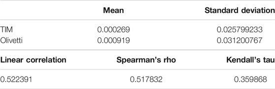
TABLE 1. Main statistics of the empirical distribution of the log-returns of TIM and Olivetti.

FIGURE 1

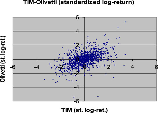
FIGURE 1. Plot of the empirical standardized log-returns TIM/Olivetti.

We have estimated, with the CML method, the parameters of different types of the bivariate copula, using the dataset of 1,012 historical daily log-returns observations. In this way, we do not consider any particular analytical form for the marginal distributions, and only the copula effects are taken into account.

Therefore, we have selected the copula which better approximates the empirical copula using the L² norm (Eq. 11). The results are shown in Table 2.

TABLE 2

TABLE 2. CML estimation of the parameters (α or R₁₂) and calculation of the L² norm for different copula types.

Observing the results in Table 2, the t₁₀-Student copula seems to be the one that better approximates the empirical copula of the dataset. However, the difference between the t₁₀-Student copula and the Normal copula is very low. So the Gaussian copula could be appropriate. We remember that the use of the Gaussian copula permits us to construct algorithms to simulate scenarios from a multivariate distribution with different margins. The commonly used multivariate Normal is only a particular case where all the margins are Gaussians too.

The simulation algorithms shown in Selecting the Right Copula Section are applied for simulating 1,000 scenarios for the standardized log-returns of the equities TIM and Olivetti, using the parameter estimations in Table 2. In all the cases, we have used standardized Gaussian margins, because our aim is only to compare the different copulas. In Figures 2–8 we have plotted the results.

FIGURE 2

FIGURE 2. 1,000 Monte Carlo simulations of bivariate random variates (x₁, x₂) with Gaussian copula (R₁₂ = 0.53248) and standard normal margins.

FIGURE 3

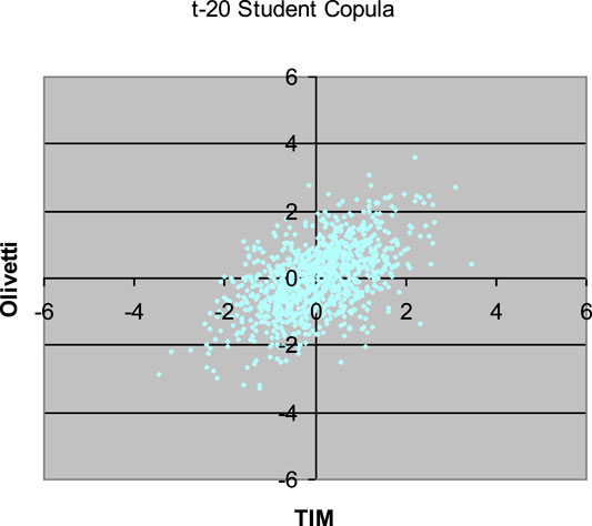
FIGURE 3. 1,000 Monte Carlo simulations of bivariate random variates (x₁, x₂) with t₂₀-Student copula (R₁₂ = 0.53564) and standard normal margins.

FIGURE 4

FIGURE 4. 1,000 Monte Carlo simulations of bivariate random variates (x₁, x₂) with t₁₀-Student copula (R₁₂ = 0.54037) and standard normal margins.

FIGURE 5

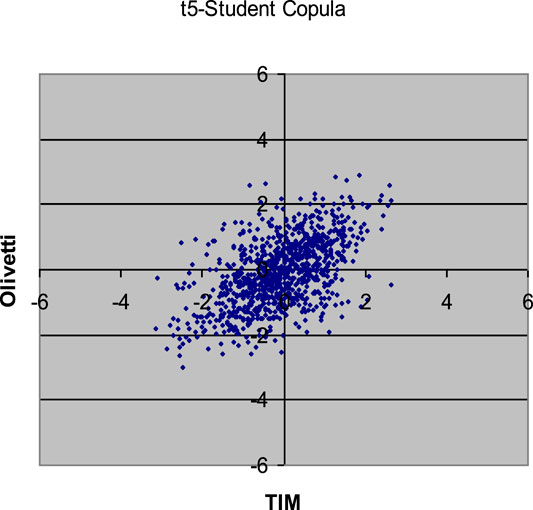
FIGURE 5. 1,000 Monte Carlo simulations of bivariate random variates (x₁, x₂) with t₅-Student copula (R₁₂ = 0.53953) and standard normal margins.

FIGURE 6

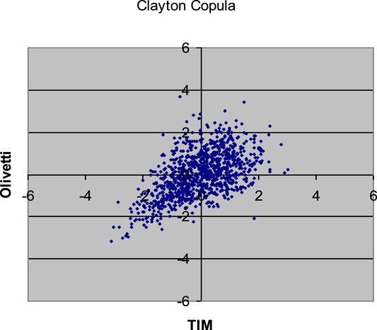
FIGURE 6. 1,000 Monte Carlo simulations of bivariate random variates (x₁, x₂) with Clayton copula (α = 1.12436) and standard normal margins.

FIGURE 7

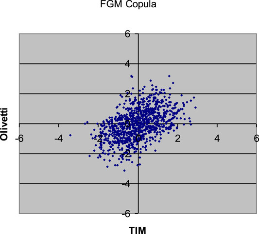
FIGURE 7. 1,000 Monte Carlo simulations of bivariate random variates (x₁, x₂) with Farlie-Gumbel-Morgenstern copula (α = 1.55349) and standard normal margins.

FIGURE 8

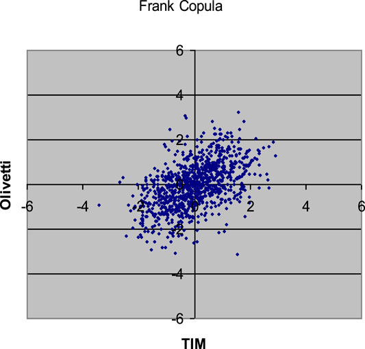
FIGURE 8. 1,000 Monte Carlo simulations of bivariate random variates (x₁, x₂) with Frank copula (α = 3.82211) and standard normal margins.

Comparing the plots in the above Figures with the empirical distribution obtained from the historical data and represented in Figure 1, we can see some differences. These deviations may be caused by an inadequate choice of the margins²¹. Our aim was only to compare different types of copulas without assumptions about the analytical form of the marginal distributions.

Concluding Remarks

This paper is a brief review of the existing methodologies for calibrating, choosing, and simulating different types of copula functions. The described methods are applied to a historical log-returns dataset of two Italian equities. We have seen how copula functions are a useful tool for implementing efficient simulation algorithms. Practical algorithms for generating Monte Carlo scenarios from a multivariate distribution with a fixed copula and different margins are easily implemented to simulate financial asset returns. The traditional models use the multinormal distribution²² to simulate asset log-returns. We can choose different marginal distributions for building more efficient algorithms also using a normal copula. The choice of the margins seems to have a more significant impact than the choice of the type of the copula on the results of the simulation. In this paper, only the copula effects are taken into account.

As clearly underlined in the paper, the application to a return time series of two Italian equities has only a demonstrative scope. The copula functions may be implemented to a portfolio of n financial assets traded on different stock markets such as the American, European and Asian ones.

In the field of portfolio risk management, the copula functions are precious tools for developing advanced financial risk measurement models. Traditionally, these quantitative instruments have been utilized for measuring more adequately the market, credit, and operational risks of financial institutions. Successively, copula functions have been also implemented in the field of the integrated measurement of the different financial risks by modeling the dependence structure among the market, credit, and operational losses. Currently, the copula functions are used for estimating the marginal contribution of each financial institution to the systemic risk, that is the instability of the global financial system. The implications in terms of macro-prudential policy and supervisory choices on financial institutions are evident.

Data Availability Statement

The raw data supporting the conclusion of this article will be made available by the authors, without undue reservation.

Author Contributions

All authors listed have made a substantial, direct, and intellectual contribution to the work and approved it for publication.

Conflict of Interest

The authors declare that the research was conducted in the absence of any commercial or financial relationships that could be construed as a potential conflict of interest.

Footnotes

¹i.e.: the class of the elliptical copulas and the class of the Archimedean copulas.

²The original definition is given by Sklar (1959) [31–33].

³For the proof, see Sklar (1996) [32].

⁴See Eqs. 1 and 2.

⁵As one can easily deduce from (Eq. 2).

⁶If $\nu \le 2$, then the covariance matrix is not defined.

⁷Y has an n-dimensional normal distribution with mean vector 0 and covariance matrix R.

⁸All the margins are equally distributed.

⁹Clayton (1978) [33].

¹⁰Gumbel (1960) [34], Hougaard (1986) [35].

¹¹Frank (1979) [36].

¹²It is a multivariate extension of the Clayton copula.

¹³Joe and Xu (1996) [13].

¹⁴In other words, the variates $({\widehat{u}}_1^t,\dots ,{\widehat{u}}_n^t)$ are generated from the empirical copula.

¹⁵See [7].

¹⁶See [4].

¹⁷i.e. the rank correlation coefficients: the Spearman’s rho, ρ_S, and the Kendall’s tau, τ.

¹⁸See [7].

¹⁹The exponential distribution has the following form: $F(x;\lambda )=1-e^{-\lambda x},x>0$.

²⁰Introduced by [12].

²¹Standardized Gaussians.

²²i.e. Gaussian copula and margins.

References

1. Li, DX. On default correlation: a Copula function approach. J Fixed Income (2000). 9:43–54. doi:10.3905/jfi.2000.319253

CrossRef Full Text | Google Scholar

2. Embrechts, P, McNeil, AJ, and Straumann, D. Correlation and dependence in risk management: properties and pitfalls In MAH Dempster, editor. Value at risk and beyond. Cambridge, UK: Cambridge University Press (2002). p. 176–223.

CrossRef Full Text | Google Scholar

3. Alexander, C. Market models: a guide to financial data analysis. London: Wiley (2001).

4. Bouyé, E, Durrleman, V, Nikeghbali, A, Riboulet, G, and Roncalli, T. Copulas for finance—a reading guide and some applications, Groupe de Recherche Opérationnelle, Crédit Lyonnais, Working Paper (2001).

Google Scholar

5. Bouyé, E, Durrleman, V, Nikeghbali, A, Riboulet, G, and Roncalli, T. Copulas: an open field for risk management. Groupe de Recherche Opérationnelle, Crédit Lyonnais, Working Paper (2000).

Google Scholar

6. Cook, RD, and Johnson, ME. A family of distributions for modeling non-elliptically symmetric multivariate data, J R Stat Soc B (1981). 43:210–8. doi:10.1111/j.2517-6161.1981.tb01173.x

CrossRef Full Text | Google Scholar

7. Durrleman, V, Nikeghbali, A, and Roncalli, T. Which copula is the right one?, Groupe de Recherche Opérationnelle, Crédit Lyonnais, Working Paper (2000).

Google Scholar

8. Embrechts, P, Hoeing, A, and Juri, A. Using copulae to bound the Value-at-Risk for functions of dependent risks, Finance and Stochastics, New York: Springer (2003).

9. Embrechts, P, Lindskog, F, and McNeil, AJ. Modelling dependence with copulas and applications to risk management. In: “Handbook of heavy-tailed distributions in finance, Chapter 8”, S Rachev, editor. Amsterdam: Elsevier (2003). p. 329–84.

CrossRef Full Text | Google Scholar

10. Frees, EW, and Valdez, EA. Understanding relationships using copulas, North Am Actuarial J. (1998). 2:1–25. doi:10.1080/10920277.1998.10595667

CrossRef Full Text | Google Scholar

11. Frey, R, and McNeil, AJ (2001). Modelling dependent default, ETH Zurich preprint.

Google Scholar

12. Genest, C, and MacKay, J. The joy of copulas: bivariate distributions with uniform marginals. Am Stat (1986). 40:280–3. doi:10.2307/2684602

CrossRef Full Text | Google Scholar

13. Genest, C, and Rivest, L-P. Statistical inference procedures for bivariate Archimedean copulas, J Am Stat Assoc (1993). 88:1034–43. doi:10.1080/01621459.1993.10476372

CrossRef Full Text | Google Scholar

14. Joe, H, and Xu, JJ. The estimation method of inference functions for margins for multivariate models. Department of statistics, University of British Columbia, Technical Report N (1996).

Google Scholar

15. Nelsen, R. An introduction to Copulas. New York: Springer (1998).

16. Oakes, D. (1982). A model for association in bivariate survival data. J R Stat Soc B 44:414–22. doi:10.1111/j.2517-6161.1982.tb01222.x

CrossRef Full Text | Google Scholar

17. Roncalli, T. Gestion des Risques Multiples, Cours ENSAI de 3ème année, Groupe de Recherche Opérationnelle, Crédit Lyonnaise (2002).

Google Scholar

18. Wang, SS. Aggregation of correlated risk portfolios: models & algorithms, CAS Committee on Theory of Risk, Working Paper (1999).

Google Scholar

19. Markowitz, H. Portfolio selection. J Finance (1952). 7:77–91. doi:10.1111/j.1540-6261.1952.tb01525.x

CrossRef Full Text | Google Scholar

20. Di Clemente, A, and Romano, C. Measuring and optimizing portfolio credit risk: a copula-based approach. Econ Notes by Banca Monte dei Paschi di Siena SpA (2004). 33(no. 3):325–57. doi:10.1111/j.0391-5026.2004.00135.x

CrossRef Full Text | Google Scholar

21. Breymann, W, Dias, A, and Embrechts, P. Dependence structures for multivariate high-frequency data in finance. Q. Finance (2003). 3(2):1–14. doi:10.1080/713666155

CrossRef Full Text | Google Scholar

22. Daul, S, De Giorgi, E, Lindskog, F, and McNeil, AJ. The grouped t-copula with an application to credit risk. Risk (2003). 16:73–6.

Google Scholar

23. Cherubini, U, Luciano, E, and Vecchiato, W. Copula methods in finance. New York: John Wiley (2004).

CrossRef Full Text

24. Demarta, S, and McNeil, AJ. The t Copula and related Copulas, working paper. Zurich: ETH Zentrum (2004).

25. Bouyé, E, and Salmon, M. Dynamic copula quantile regressions and tail area dynamic dependence in Forex markets. Eur J Finance (2009). 15:721–50. doi:10.1080/13518470902853491

CrossRef Full Text | Google Scholar

26. Hakwa, B, Jager-Ambrozewicz, M, and Rudiger, B. Analysing systemic risk contribution using a closed Formula for conditional valueat-risk through copula. Commun Stoch Anal (2015). 9(1):131–58. doi:10.31390/cosa.9.1.08

CrossRef Full Text | Google Scholar

27. Karimalis, EN, and Nomikos, NK. Measuring systemic risk in the European banking sector: a Copula CoVaR approach. Eur J Finance (2018). 24(11):944–75. doi:10.1080/1351847x.2017.1366350

CrossRef Full Text | Google Scholar

28. Di Clemente, A. Estimating the marginal contribution to systemic risk by a CoVaR-model based on copula functions and ExtremeValue Theory. Finance Monet Econ (2018). 47(1):69–112. doi:10.1111/ecno.12095

CrossRef Full Text | Google Scholar

29. Gauthier, C, Lehar, A, and Souissi, M. Macroprudential capital requirements and systemic risk. J Financial Intermediation (2012). 21(4):594–618. doi:10.1016/j.jfi.2012.01.005

CrossRef Full Text | Google Scholar

30. Di Clemente, A. Comparing different systemic risk measures for European banking system. Int Bus Res (2019). 12:35–53.

Google Scholar

31. Sklar, A. Fonctions de répartition à n dimensions et leurs marges. Publications de l’Institut de Statistique de l’Université de Paris (1959). 8:229–31.

Google Scholar

32. Sklar, A. (1996). : Random variables, distribution functions, and copulas – a personal look backward and forward, in Distributions with fixed marginals and related topics, ed. By L Rüschendorff, B Schweizer, and M Taylor. Hayward, CA: Institute of Mathematical Statistics, pp. 1–14.

CrossRef Full Text

33. Clayton, DG. A model for association in bivariate life tables and its application in epidemiological studies of familial tendency in chronic disease incidence. Biometrika (1978). 65:141–51. doi:10.1093/biomet/65.1.141

CrossRef Full Text | Google Scholar

34. Gumbel, EJ. Bivariate exponential distributions. J Am Stat Assoc (1960). 55:698–707. doi:10.1080/01621459.1960.10483368

CrossRef Full Text | Google Scholar

35. Hougaard, P. A class of multivariate Failure time distributions. Biometrika (1986). 73:671–8. doi:10.2307/2336531

CrossRef Full Text | Google Scholar

36. Frank, MJ. On the simultaneous associativity of F(x, and x+y-F(x,y). Aequationes Mathematicae (1979). 19:194–226. doi:10.1007/bf02189866

CrossRef Full Text | Google Scholar

37. Mashal, R, and Zeevi, A. “Beyond Correlation: extreme Co-movements between financial assets”. Working Paper: Columbia University (2002).

38. Deheuvels, P. La fonction de dépendance empirique et ses propriétés – un test non paramétrique d’indépendance. Académie Royale de Belgique – Bulletin de la Classe des Sciences – 5e Série. N. (1979). 65:274–92. doi:10.3406/barb.1979.58521

CrossRef Full Text | Google Scholar

39. Marshall, AW, and Olkin, I. Families of multivariate distributions. J Am Stat Assoc (1988). 84:487–93.

Google Scholar

40. Johnson, ME. Multivariate statistical simulation. New York: Wiley (1987).