Intensity Estimation for Poisson Process With Compositional Noise

1. Introduction

The study of point processes is one of the central topics in stochastic processes and has been widely used to model discrete events in continuous time. In particular, the Poisson process, a common point process, has the most applications [1–3]. Classical examples include the arrivals of park patrons at an amusement park over a period of time, the goals scored in an association football match, and the clicks on a particular web link in a given time period. Recently, Poisson processes have been used to characterize spiking activity in various neural systems [4, 5]. In order to use a Poisson process in applications, one key step is to estimate its intensity function from a given sequence of observed events.

The estimation of the intensity of a Poisson process has been studied extensively and various methodologies have been proposed. If the intensity can be assumed to have a known parametric form, then likelihood-based methods can be used to estimate the model parameters [6]. However, in many cases, the shape of the intensity is unknown and estimation requires the implementation of non-parametric methods. Indeed, non-parametric estimations provide more flexibility than parametric methods and can better characterize the underlying intensity function. A number of approaches have been proposed over the past three decades, including wavelet-based methods [2, 7, 8] and kernel-based methods [1, 9, 10]. In the case where prior knowledge about the process or shape of the intensity is known, Bayesian methods can be adopted and they often lead to a more accurate estimation [11–13].

Treating a neural spike train as a realization of Poisson process, one can consider the example depicted in Figure 1. In this case, the neural spiking activity, associated with certain movement behavior [14], was recorded (see detail of the data in section 3.3). The process was repeated for 30 trials and the resulting spike trains are shown in Figure 1A. Notice that in each repetition of the same movement, there is a gap in the spikes that occurs at slightly different times with variable lengths. This time shift in the gap in spikes is indeed an example of the notion of phase variability or compositional noise, a central topic in functional data analysis. The observed gap in spikes should be reflected in the underlying Poisson intensity estimate. However, using kernel-based estimation methods without accounting for phase variability results in an intensity estimate (shown in red in Figure 1B) that does not capture this gap in spiking activity. The method introduced later in this paper does consider the presence of phase variability and yields an estimate of the underlying intensity of the spike train that clearly depicts the observed gap in the spiking activity (shown in blue in Figure 1B). Therefore, it is important to develop estimation procedures that consider the presence of phase variability in repeated observations of the same process.

FIGURE 1

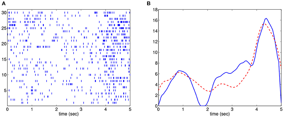
Figure 1. Intensity estimation example. (A). 30 spike train observations. (B). Estimated intensities by considering (solid blue) and not considering (dashed red) compositional noise.

One key concept in functional data analysis where phase variability plays the central role is the notion of function registration, or alignment. Indeed, function registration is an important topic in functional data analysis and a significant amount of research progress has been made over the past two decades [15–19]. In order to properly register functions, one must consider two types of variability present in data: phase and amplitude variability. Phase variability describes the degree of “unalignment” in the data, and amplitude variability is the remaining variability in the vertical axis after alignment. The goal of function registration is to align the functions by removing phase variability. If analysis (such as principal component analysis or regression) is conducted on data which are not well aligned, one may obtain poor or undesired results.

While function registration has been extensively investigated, the notion of aligning point processes with compositional noise has not been well studied — all aforementioned intensity estimation methods are based on the assumption there is no phase variability in the observed processes. However, as indicated in the above spike train example, that is not always a reasonable assumption. To understand the phase variability in point process observations, recent studies on intensity estimation in Poisson process have begun to identify and remove compositional noise during the estimation procedure. For example, Bigot and colleagues examined the estimation of the underlying intensity function for a set of linearly shifted Poisson processes [20]. They assumed that the intensity function is periodic and each realization of the process is warped according to a linear shift in time that follows a known distribution. Under the stated assumptions, the authors derived a wavelet-based estimator. They argued that the assumption of a linear shift in the observed processes is a reasonable assumption, particularly in an example of DNA Chip-Seq data. However, there are many other cases where it is not reasonable to assume a simple linear shift for the phase variability such as examples in [15, 19]. As a result, restricting the warping function to be strictly linear shifts may limit the general applicability of their method. In another recent study, Panaretos and Zemel proposed to separate amplitude and phase variation in order to align point processes [21]. Basically, they extended the notion of the separation of phase and amplitude variation in functions to that of point processes. We point out that Panaretos and Zemel's work focues on estimation of the probability measure and not for density estimation [see section 3.4 of [21]]. In contrast, our goal in this study is clearly intensity estimation.

In this paper we propose a new framework for intensity estimation of a Poisson process with compositional noise. We show that the noise is only encoded in the normalized intensity, or density, function. The estimation is based on our proposed metric which measures the phase difference between two density functions so the notion of the Karcher mean can be applied in the given framework. Since the only parameter in the method is the bandwidth for the kernel density estimate, the proposed method is still non-parametric.

A recent study on Poisson process with compositional noise adopts the generalized linear model (GLM) where the phase noise is addressed by the well-known Dynamic Time Warping (DTW) method [6]. We point that the goals and approaches in our paper and this GLM-DTW study are very different:

1. In our study, we assume the observed point processes are random samples (with phase variability) from a Poisson process and there is no other co-variate. In contrast, the GLM-DTW study adopts a GLM framework — conditioned on some covariates, the process is Poisson. These co-variates are needed for encoding/decoding purposes.

2. Our goal is to esimate the deterministic intensity function from these given samples. In contrast, the GLM-DTW study focuses on building proper model between point process observations and underlying covariates.

3. We conduct warping transformation in the velocity space which is an area-preserving procedure (see detail in section 2.1.1). This invariance will preserve the probability for the total number of events in the process, a critical measure for the non-linear transformation within the time domain. In contrast, the GLM-DTW study does not have such invariance in its framework, which often leads to a degenerate estimate.

The rest of this paper is organized as follows. In section 2, we present the new framework for positive and non-negative intensity estimation and discuss its mathematical and computational properties. Consistency theory on the estimation algorithm is also examined. The estimations on positive and non-negative intensity are illustrated with two simulations, respectively, in section 3. We then show the application of intensity estimation in a real dataset of neural spike trains. Section 4 summarizes the work. Finally, all mathematical details are given in the Appendices.

2. Methods

In this section, we present the new framework for intensity estimation of a Poisson process with non-linear time warping.

2.1. Positive Intensity Estimation

We will at first focus on positive intensity functions, where compositional noise is represented with time warping. We will review the basics of Poisson processes [22] and the representation of time warping in function space [23].

2.1.1. Review of Poisson Process and Time Warping Representation

A Poisson process on the time domain [0, 1] is a special type of counting process N(t), t ∈ [0, 1]. For simplification of notation, we only examine the domain [0, 1] in this paper, and the framework can be easily adapted to any finite time interval. In the classical theory of point processes, a Poisson process is defined based on an intensity function λ(t) ≥ 0 and satisfies the following two conditions [22]:

1. Disjoint intervals have counts that are independent.

2. The number of events in an interval (a, b) ⊂ [0, 1] follows a Poisson distribution with mean ${\int }_a^b\lambda (t)dt$.

We denote a Poisson process with intensity λ(t) as PP(λ(t)). For distinction, a Poisson distribution with mean μ is denoted as Poisson(μ), and a Poisson probability mass function with mean μ at k is denoted as Poisson(k; μ) = e^−μμ^k/k!.

We represent compositional noise with time warping functions. Since the intensity of a Poisson process is a function, we study the representation of time warping in the function space. Let Γ be the set of all warping functions, where time warping is defined as an orientation-preserving diffeomorphism of the domain [0, 1]. That is,

$\Gamma =\left\{\gamma :\left[0,1\right]\to \left[0,1\right]|\gamma (0)=0,\gamma (1)=1,0<\dot{\gamma }<\infty \right\}.$

Elements of Γ form a group with function composition as the group action, and the identity in this group is the self-mapping γ_id(t) = t. For any function h ∈ 𝕃²([0, 1]), we will use ‖h‖ to denote its 𝕃² norm ${({\int }_0^{1}h{(t)}^{2}dt)}^{1/2}$.

There are three different types of (right) group actions about time warping that can occur in the function space:

1. Amplitude-preserved: f → f ∘ γ,

2. Area (𝕃¹ norm)-preserved: $f\to (f\circ \gamma )\dot{\gamma }:=(f;\gamma )$,

3. Energy (𝕃² norm)-preserved: $f\to (f\circ \gamma )\sqrt{\dot{\gamma }}:=(f,\gamma )$,

where ∘ denotes the conventional function composition. The properties on associativity and isometry of these three group actions are summarized in Table 1. In particular, the amplitude-preserved group action is the conventional registration for functions with phase variability and has been extensively studied over the past two decades [24–26]. The enery-preserved group action plays an essential role in the Fisher-Rao registration framework [27], where this action is applied in the Square-Root Velocity Function (SRVF) space (note: it is critical that in the Fisher-Rao framework there is a one-to-one correspondence between the energy-preserved SRVF space and the amplitude-preserved observational function space). In the following sections of this paper, we will show that the compositional noise in the Poisson process intensity function is properly characterized by the area-preserved group action.

TABLE 1

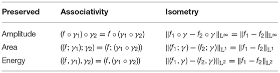
Table 1. Properties of the three group actions.

2.1.2. Poisson Process With Compositional Noise

Before formally stating the main problem, we review the classical estimation problem in Poisson processes: Given a set of independent realizations from a Poisson process on [0, 1], how can we estimate the underlying intensity function? By notation, the set of realizations are given in the following form,

$R^i=(r_1^i,\cdots ,r_{k_i}^i)~PP(\lambda (t)),$

where $k_i~Poisson\left({\int }_0^1\lambda (t)dt\right),i=1,2,\dots ,n$. Various approaches have been developed to address this problem, which include penalized projection estimators [28], wavelet methods [7, 29], and estimators based upon thresholding rules [8].

In this paper, we assume the observed data are not {Rⁱ}, but a warped version in the form

$S_i=(s_1^i,\cdots ,s_{k_i}^i)={\gamma }_i^{-1}(R^i)=({\gamma }_i^{-1}(r_1^i),\cdots ,{\gamma }_i^{-1}(r_{k_i}^i)),$

where γ_i is a random time warping in Γ, i = 1, ⋯ , n. That is,

$\begin{array}{ll}{S}_i={\gamma }_i^{-1}(R^i),\text{with }{R}^i~PP(\lambda (t)),{\gamma }_i\in \Gamma .& (1)\end{array}$

Given observations {S_i}, our goal is still to estimate the underlying intensity λ(t). To make the model identifiable, we add a constraint that the mean of {γ_i} needs to be a scaled version of γ_id (The detail on assumptions is clearly provided in section 2.2). Since the time warping can be in any non-linear form, this estimation problem is a significant challenge. A recent study only examines the case when the warping is a simple linear shift along the time axis [20].

As the warping function γ_i is random, the warped process ${\gamma }_i^{-1}(R_i)$ is no longer a Poisson process, but a Cox process. Here we study, “Conditional on γ_i, is ${\gamma }_i^{-1}(R^i)$ still a Poisson process? If this is true, what is the intensity function of that Poisson process?” Our answer is yes to the first question and the intensity function of the new Poisson process is given as follows.

Lemma 1. Suppose R is a Poisson process with intensity λ(t) on [0, 1] and γ ∈ Γ is a given time warping function. Then γ⁻¹(R) is also a Poisson process with intensity $\lambda (\gamma (t))\dot{\gamma }(t).$

Proof: If R is a Poisson process, then the number of events of R in the time interval (a, b) is independent of the number of events of R in the time interval (c, d) if (a, b) ∩ (c, d) = ∅. Since γ(t) is strictly increasing, (a, b) ∩ (c, d) = ∅ ⇔ (γ (a), γ (b)) ∩ (γ (c), γ (d)) = ∅. Hence, the number of events in (γ (a), γ (b)) is also independent of the number of events in (γ (c), γ (d)).

For any k ∈ {0, 1, ⋯ } and sub-interval [t, t + Δt] ⊂ [0, 1],

$\begin{array}{l}P(k\text{ events of }{\gamma }^{-1}(R)\text{ are in }[t,t+\Delta t])\\ =P(k\text{ events of }R\text{ are in }[\gamma (t),\gamma (t+\Delta t)])\\ =Poisson\left(k;\stackrel{\gamma (t+\Delta t)}{\underset{\gamma (t)}{\int }}\lambda (v)dv\right)\\ =Poisson\left(k;\stackrel{t+\Delta t}{\underset{t}{\int }}\lambda (\gamma (u))\dot{\gamma }(u)du\right).\end{array}$

The last equality holds simply by the change of variable v = γ (u). Therefore,

${\gamma }^{-1}(R)~PP\left(\lambda (\gamma (u))\dot{\gamma }(u)\right).$

A direct result from Lemma 1 is that given γ_i, S_i is also a Poisson process and

$S_i|{\gamma }_i={\gamma }_i^{-1}(R^i)|{\gamma }_i~PP(\lambda ({\gamma }_i(t)){\dot{\gamma }}_i(t)).$

Based on the theory of Poisson processes, the intensity function λ(t) can be decomposed into the product of the total intensity Λ and the density function f(t), where

$\Lambda ={\displaystyle {\int }_0^1}\lambda (t)dt\text{and }f(t)=\lambda (t)/\Lambda .$

Therefore, the intensity estimation problem can be reduced to density estimation and scalar total intensity estimation.

Note that for i = 1, ⋯ , n,

${\displaystyle {\int }_0^1}{\lambda }_i(t)dt={\displaystyle {\int }_0^1}\lambda ({\gamma }_i(t))\dot{\gamma }(t)dt={\displaystyle {\int }_0^1}\lambda (s)ds=\Lambda .$

That is, Λ is constant with respect to time warping and the intensity function is area-preserved with respect to compositional noise. Hence, the density of the events in S_i, given γ_i, can be written as $f_i(t)={\lambda }_i(t)/\Lambda =\lambda ({\gamma }_i(t)){\dot{\gamma }}_i(t)/\Lambda$. This expression indicates that the time warping is encoded in the density function, and independent of total intensity. By the theory of Poisson processes, the number of events in each process follows a Poisson distribution with mean Λ. For a set of given observations {S_i}, Λ can be easily estimated using a conventional maximum likelihood estimate. Therefore, the intensity estimation problem reduces to estimating the underlying density f. Given {S_i}, we propose a modified kernel method to estimate density functions {f_i}, and then use these densities to estimate f. This whole procedure is described in detail in section 2.1.5.

2.1.3. Phase Distance Between Positive Probability Density Functions

In this paper, we focus on a metric-based method to estimate the underlying density f. Metric distances between density functions is a classical topic and a number of measures have been proposed, for example, the Bhattacharyya Distance [30], the Hellinger Distance [31], the Wasserstein Distance [32], and the elastic distance beween densities based upon the Fisher-Rao metric [33]. Suppose f₁ and f₂ are two density functions on [0,1] with cumulative distribution functions F₁ and F₂, respectively. Then, these metrics are defined as:

• Wasserstein Distance: $d_W(f_1,f_2)=\Vert F_1^{-1}-F_2^{-1}\Vert$

• Bhattacharyya Distance: $d_B(f_1,f_2)=-\log \left(\int \sqrt{f_1(t)f_2(t)}dt\right)$

• Hellinger Distance: $d_H(f_1,f_2)=\frac{1}{\sqrt{2}}\Vert \sqrt{f_1}-\sqrt{f_2}\Vert$

• Fisher-Rao Distance: $d_{FR}(f_1,f_2)=arccos\left({\int }_0^1\sqrt{f_1(t)}\sqrt{f_2(t)}dt\right)$

Note that the Fisher-Rao metric between two density functions is similar to the Hellinger Distance (arc length vs. chord length) [33].

Based on the generative model in Equation (1), the difference between the true underlying density function and the noise-contaminated density is the time warping along the time axis. Such a difference is characterized as the phase difference and we expect that a metric measuring phase difference will be purely based on the warping function between two densities. That is, the distance between f₁ and f₂ will only depend on γ if f₁ = (f₂; γ). However, none of the above metrics purely measure this phase difference between two density functions. We aim to find a metric that can properly characterize such phase difference. In this paper, we will define a new distance between positive densities which properly measures their phase difference. The set of all positive density functions on [0, 1] is denoted as ℙ.

We note that for any densities f₁, f₂ ∈ ℙ, their cumulative distribution functions F₁, F₂ are warping functions in Γ. By the group structure of Γ, it is straightforward to find that the optimal warping function between f₁ and f₂ (i.e., γ^* ∈ Γ such that $f_1=(f_2\circ {\gamma }^{*}){\dot{\gamma }}^{*}$ or $F_1=F_2\circ {\gamma }^{*}$), is unique and has a closed-form solution given by

$\begin{array}{ll}{\gamma }^{*}=F_2^{-1}\circ F_1.& (2)\end{array}$

Based on this result, it is natural to define a distance that measures the phase difference by measuring how far the warping function is from the identity warping function, γ_id. In other words, the smaller the distance between the warping function and γ_id, the less warping that is required between the two densities. One definition of the distance metric is given as follows.

Definition 1. For any two functions f₁, f₂ ∈ ℙ, we define an intrinsic distance, d_int, between them as:

$\begin{array}{ll}{d}_{int}(f_1,f_2)=\arccos \langle 1,\sqrt{\dot{\gamma }}\rangle & (3)\end{array}$

where γ is the optimal time warping between f₁ and f₂ (i.e., $f_1=(f_2\circ \gamma )\dot{\gamma }$).

This definition of phase distance has been used in the Fisher-Rao framework [19]. This distance is intrinsic which measures the arc-length between $\sqrt{\dot{\gamma }}$ and 1 in the unit sphere S^∞ (SRVF space of Γ). Note that the definition of phase distance in ℙ is not unique. We can also define an extrinsic distance as follows:

Definition 2. For any two functions f₁, f₂ ∈ ℙ, we define an extrinsic distance, d_ext, between them as:

$\begin{array}{ll}{d}_{ext}(f_1,f_2)=\Vert 1-\sqrt{\dot{\gamma }}\Vert & (4)\end{array}$

where γ is the optimal time warping between f₁ and f₂ (i.e., $f_1=(f_2\circ \gamma )\dot{\gamma }$).

Notice that because the optimal warping function $\gamma =F_2^{-1}\circ F_1$, the distance d_ext(f₁, f₂) can also be written as $\Vert 1-\sqrt{F_2^{-1}\dot{○}{F}_1}\Vert =\Vert \sqrt{{\dot{F}}_1^{-1}}-\sqrt{{\dot{F}}_2^{-1}}\Vert$. The commonly-used Wasserstein distance d_W is

$d_W(f_1,f_2)=\Vert F_1^{-1}-F_2^{-1}\Vert \le 2\Vert \sqrt{{\dot{F}}_1^{-1}}-\sqrt{{\dot{F}}_2^{-1}}\Vert =2d_{ext}(f_1,f_2)$

This shows that the consistency results that hold for d_ext will also hold for d_W, but the reverse is not true in general. Similar to the Wasserstein and Hellinger distances, this d_ext metric is also a proper distance. The detailed proof in given in Appendix A. While d_ext is not isometric like Bhattcharya and Hellinger, it is the only metric (within these four) that specifically characterizes the phase difference between f₁ and f₂.

Either d_int or d_ext can be used to estimate the underlying density f. In this paper, we choose to focus on the extrinsic distance d_ext for two reasons: (1) Computational algorithms based upon the extrinsic distance are usually more efficient than those based on the intrinsic distance. (2) The extrinsic distance provides a closed-form Karcher mean representation (see the definition next), which plays an essential role in developing the asymptotic theory for our estimator in section 2.2.

2.1.4. Karcher Mean

The notion of the Karcher mean was used on the set of warping functions where an extrinsic distance between warping functions is adopted [14]. That is, assuming γ₁, ⋯ , γ_n ∈ Γ is a set of warping functions, their Karcher mean $\bar{\gamma }$ can be defined as

$\bar{\gamma }=\underset{\gamma \in \Gamma }{\arg \min }{\displaystyle \sum _{i=1}^n}\Vert \sqrt{\dot{\gamma }}-\sqrt{{\dot{\gamma }}_i}{\Vert }^2.$

It was shown in [14] that this Karcher mean has a closed-form solution:

$\sqrt{\dot{\overline{\gamma }}}=\frac{{\displaystyle {\sum }_{i=1}^n\sqrt{{\dot{\gamma }}_i}}}{\Vert {\displaystyle {\sum }_{i=1}^n\sqrt{{\dot{\gamma }}_i}}\Vert },$

where $\sqrt{\stackrel{\bullet }{\bar{\gamma }}}$ is the SRVF of $\bar{\gamma }$.

Similar to the Karcher mean of a set of warping functions in Γ, we can define the Karcher mean of a set of density functions in ℙ. This definition is based on the newly-defined phase distance d_ext in Equation (4).

Definition 3. We define the Karcher mean μ_n of functions f₁, ⋯ , f_n ∈ ℙ as the minimum of the sum of squares of distances in the following form:

$\begin{array}{ll}{\mu }_n=\underset{\mu \in \mathbb{P}}{\arg \min }{\displaystyle \sum _{i=1}^n{d}_{ext}}{(\mu ,f_i)}^2.& (5)\end{array}$

Based on the closed-form solution for the Karcher mean of a set of warping functions, we can efficiently compute the Karcher mean in Equation (5) using the following algorithm.

ALGORITHM 1

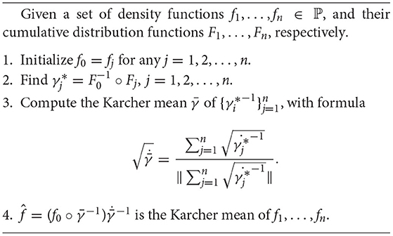
Algorithm 1: Karcher Mean Computation.

The algorithm for computing the Karcher mean of functions in ℙ is illustrated with a simple example in Figure 2. The 10 yellow lines in the figure denote the density functions of Beta distribution on the domain [0, 1] in the form f(x; α, β) ∝ x^α−1(1 − x)^β−1. Here the parameters α takes value 1, 1, 1.5, 2, 2, 2.5, 3, 3, 4, 5, and β takes value 4, 3, 3, 2.5, 2, 2, 1.5, 1, 1, 2 for the 10 functions, respectively. The Karcher mean of these functions was computed using Algorithm 1 and the result is shown as the thick red line in the figure.

FIGURE 2

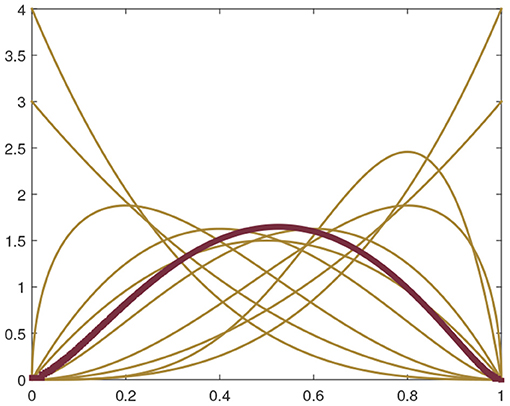
Figure 2. Karcher mean of 10 Beta density functions.

2.1.5. Intensity Estimation Method

Since the Karcher mean of a set of density functions (computed under d_ext) is itself a density function, we use the Karcher mean as an estimate of the underlying density of the process. In our proposed estimation method, the Karcher mean, as computed using Algorithm 1, is used in conjunction with the MLE of the total intensity of the process to produce an estimate of the intensity function. Note that the computation for Karcher mean using Algorithm 1 is based on the assumption that each warped density f_i(t) is already known, but practical data are only Poisson process realizations. In this section, we propose a kernel estimation procedure to estimate f_i(t).

Modified Kernel Density Estimation: Kernel density estimation has been well studied in statistics literature and it is well known that the standard kernel density estimator has good asymptotic properties when the domain is the real line. However, when the domain is a compact set such as [0, 1] in this paper, the standard kernel density estimator cannot be directly used. We adopt here a reflection-based method to address this issue [34–36].

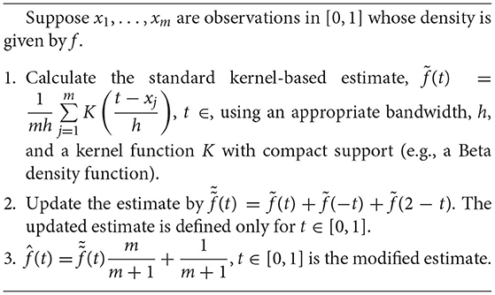
Suppose x₁, …, x_m are observations in [0, 1] whose density is given by f ∈ ℙ. The standard kernel density estimator is given by $\tilde{f}(t)=\frac{1}{mh}{\displaystyle \sum _{j=1}^{m}K\left(\frac{t-x_j}{h}\right)},$, where K(·) is a kernel function and h denotes the kernel width. Note that this estimated density is defined on the real line (−∞, ∞), and the section within [0, 1] in general is not a density function itself. To simplify the estimation procedure, we can choose kernel functions with compact support within [−1, 1]. That is, K(t) = 0 for |t| > 1.

Here we propose a two-step modification of the estimate $\tilde{f}(t)$. At first, we wrap around $\tilde{f}$ within the domain [0, 1], and denote the new function as $\widetilde{\stackrel{~}{f}}$, a density function on [0, 1]. Secondly, we add a small positive constant to $\widetilde{\stackrel{~}{f}}$, and then normalize the sum to be a density function. This step is to assure that the normalized function is positive on [0, 1], a necessary condition for the existence of the warping functions used in the distance d_ext. The modified kernel density estimation can be summarized in the following algorithm.

ALGORITHM 2

Algorithm 2: Modified Kernel Estimation.

Estimation Algorithm: Estimation of the intensity of the process occurs in two independent components. First, the total intensity Λ can be easily computed with a standard MLE procedure. Second, the Karcher mean of the estimated densities is used to estimate f(t). This estimation algorithm is given as follows.

ALGORITHM 3

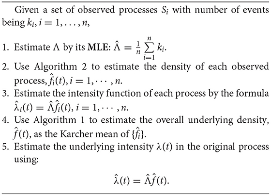
Algorithm 3: Intensity Estimation Algorithm.

2.2. Asymptotic Theory on Consistency

Asymptotic properties of estimators are often of interest since these properties provide reasonable certainty that the ground-truth parameters can be appropriately estimated by the given algorithms. In this section, we provide asymptotic theory on the density estimator $\widehat{f}$ in Algorithm 3. Our estimation is based on the model

${\lambda }_i=(\lambda \circ {\gamma }_i){\dot{\gamma }}_i,i=1,\cdots ,n,$

where λ is the underlying intensity function and γ_i ∈ Γ, i = 1, …, n, are a set of warping functions. By Lemma 1, each observation S_i is a Poisson process realization with intensity λ_i. Given {S_i}, Algorithm 3 provides an estimation procedure for λ. As the total intensity Λ is independent of time warpings, our asymptotic theory will focus on the normalized intensity, i.e., intensity function f = λ/Λ. We mathematically prove that the proposed algorithm provides a consistent estimator for f. The asymptotic theory is based on sample size n as well as the total intensity Λ. Here we only provide result on the main theorem. All lemmas that lead to the theorem can be found in Appendix B.

Before we state the main theorem, we list all assumptions as follows:

1. The observations are a sequence of Poisson process realizations {S_i}, and S_i follows intensity function ${\lambda }_i=(\lambda \circ {\gamma }_i){\dot{\gamma }}_i$. $\Lambda ={\int }_0^1\lambda (t)dt$ is the total intensity. f = λ/Λ and f_i = λ_i/Λ = (f; γ_i).

2. The density function f is continuous on [0,1]. Also, there exist m_f, M_f > 0 such that f(t) ∈ [m_f, M_f], for any t ∈ [0, 1].

3. γ_i(t), t ∈ [0, 1], i = 1, ⋯ , n are a set of independent warping functions. The SRVFs of their inverses $\sqrt{{\dot{\gamma }}_i^{-1}(t)}$ distribute around $\sqrt{{\dot{\gamma }}_{id}}=1$ on the Hilbert unit sphere H^∞. In particular, $E(\sqrt{{\dot{\gamma }}_i(t)})\equiv \beta >0$ and there exist m_γ, M_γ > 0 such that $\sqrt{{\dot{\gamma }}_i^{-1}(t)}\in \left[m_{\gamma },M_{\gamma }\right]$, for any t ∈ [0, 1]. It is important to note that $\sqrt{{\dot{\gamma }}_i^{-1}(t)}$ is a point on the Hilbert unit sphere. As a result, it is easy to show that assuming $𝔼\left(\sqrt{{\dot{\gamma }}_i^{-1}(t)}\right)=\beta >0$ is equivalent to assuming that the extrinsic mean of $\left\{\sqrt{{\dot{\gamma }}_i^{-1}(t)}\right\}$ is 1.

4. The total intensity Λ can vary in the form of a sequence ${\left\{{\Lambda }_m\right\}}_{m=1}^{\infty }$. We assume the sequence goes to ∞ with Λ_m ≥ α log(m), α > 1 for sufficiently large m.

5. The bandwidth of the kernel density estimator in Algorithm 2 is chosen optimally. That is, for a sequence of r events, the bandwidth h_r satisfies h_r → 0 and rh_r → ∞ when r → ∞.

Theorem 1. Given the five conditions listed above, let $\widehat{f}$ be the density function estimated with Algorithm 3. Then we have

${\displaystyle \underset{n\to \infty }{lim}}{\displaystyle \underset{m\to \infty }{lim}}{d}_{ext}(\widehat{f},f)=0a.s.$

Proof: By the basic property of a Poisson process, the event times in the observation S_i are an i.i.d. sequence with density function f_i = (f; γ_i), i = 1, ⋯ , n. Denote ${\widehat{f}}_i$ as the estimated density function by the modified kernel estimation method. Then ${\widehat{f}}_i(t)>0$ for any t ∈ [0, 1]. Based on the group structure of Γ, there exists a unique ${\widehat{\gamma }}_i\in \Gamma$ such that ${\widehat{f}}_i=(f;{\widehat{\gamma }}_i)$.

Here we compute the Karcher mean of $\left\{{\widehat{f}}_i\right\}$. For any density function g, we have

$\begin{array}{l}{\displaystyle \sum _{i=1}^n{d}_{ext}^2({\widehat{f}}_i,g)}={\displaystyle \sum _{i=1}^n{d}_{ext}^2((f;{\widehat{\gamma }}_i),g)}={\displaystyle \sum _{i=1}^n{\Vert \left(1,{\gamma }_{(f;{\widehat{\gamma }}_i)}^{-1}\right)-\left(1,{\gamma }_g^{-1}\right)\Vert }^2}\\ ={\displaystyle \sum _{i=1}^n{\Vert \left(1,{\widehat{\gamma }}_i^{-1}\circ {\gamma }_f^{-1}\right)-\left(1,{\gamma }_g^{-1}\right)\Vert }^2}\\ ={\displaystyle \sum _{i=1}^n{\Vert \left(1,{\widehat{\gamma }}_i^{-1}\right)-\left(1,{\gamma }_g^{-1}\circ {\gamma }_f\right)\Vert }^2}.\end{array}$

Denote the Karcher mean of $\left\{{\widehat{\gamma }}_i^{-1}\right\}$ as $\widehat{\bar{\gamma }}$. Then the above sum of squares is minimized when ${\gamma }_g^{-1}\circ {\gamma }_f=\widehat{\bar{\gamma }}$. That is, ${\gamma }_{\widehat{f}}^{-1}=\widehat{\bar{\gamma }}\circ {\gamma }_f^{-1}.$ By isometry on time warping functions and the triangular inequality,

$\begin{array}{l}{d}_{ext}(\widehat{f},f)=\Vert \left(1,{\gamma }_{\widehat{f}}^{-1}\right)-\left(1,{\gamma }_f^{-1}\right)\Vert =\Vert \left(1,\widehat{\overline{\gamma }}\circ {\gamma }_f^{-1}\right)-\left(1,{\gamma }_f^{-1}\right)\Vert \\ =\Vert \left(1,\widehat{\overline{\gamma }}\right)-1\Vert \le \Vert \left(1,\widehat{\overline{\gamma }}\right)-\left(1,\overline{\gamma }\right)\Vert +\Vert \left(1,\overline{\gamma }\right)-1\Vert .\end{array}$

By Lemma 5, we have shown that $\Vert (1,\bar{\gamma })-1\Vert \underset{}{\overset{a.s.}{\to }}0$ when n → ∞. Note that $\Vert \left(1,\widehat{\bar{\gamma }}\right)-(1,\bar{\gamma })\Vert$ depends on the total intensity Λ_m and sample size n. We will show that this term also converges to 0 when m is large (for any fixed n).

To simplify the notation, we denote $a_i=\sqrt{{\dot{\gamma }}_i^{-1}}$, ${\widehat{a}}_i=\sqrt{{\dot{\widehat{\gamma }}}_i^{-1}},i=1,\cdots ,n.$ Let the number of events in S_i be n_i. Then n_i is a random variable following Poisson distribution with mean Λ_m. By Lemma 5, $n_i\underset{}{\overset{a.s.}{\to }}\infty$ when m → ∞. Using Lemma 3,

$\begin{array}{l}\Vert {\widehat{a}}_i-a_i\Vert =\Vert (1,{\widehat{\gamma }}_i^{-1})-(1,{\gamma }_i^{-1})\Vert \\ =\Vert (1,{\widehat{\gamma }}_i^{-1}○{\gamma }_f^{-1})-(1,{\gamma }_i^{-1}○{\gamma }_f^{-1})\Vert \\ =\Vert (1,{\gamma }_{(f;{\widehat{\gamma }}_i)}^{-1})-(1,{\gamma }_{(f;{\gamma }_i)}^{-1})\Vert \\ =\Vert (1,{\gamma }_{{\widehat{f}}_i}^{-1})-(1,{\gamma }_{f_i}^{-1})\Vert \stackrel{a.s.}{\to }0\end{array}$

when n_i → ∞. Therefore, $\Vert {â}_i-a_i\Vert \underset{}{\overset{a.s.}{\to }}0,i=1,\cdots ,n,$ when m → ∞.

Let $\overline{â}=\frac{1}{n}\sum _{i=1}^n{â}_i$ and $ā=\frac{1}{n}\sum _{i=1}^n{a}_i$. Then, $\Vert \overline{â}-ā\Vert \underset{}{\overset{a.s}{\to }}0$ when m → ∞. Hence,

$\begin{array}{l}\Vert \left(1,\widehat{\overline{\gamma }}\right)-\left(1,\overline{\gamma }\right)\Vert =\Vert \frac{\overline{\widehat{a}}}{\Vert \overline{\widehat{a}}\Vert }-\frac{\overline{a}}{\Vert \overline{a}\Vert }\Vert \le \Vert \frac{\overline{\widehat{a}}}{\Vert \overline{\widehat{a}}\Vert }-\frac{\overline{\widehat{a}}}{\Vert \overline{a}\Vert }\Vert \\ +\Vert \frac{\overline{\widehat{a}}}{\Vert \overline{a}\Vert }-\frac{\overline{a}}{\Vert \overline{a}\Vert }\Vert \\ \le 2\Vert \overline{\widehat{a}}-\overline{a}\Vert /\Vert \overline{a}\Vert \stackrel{a.s.}{\to }0(\text{when }m\to \infty )\end{array}$

Note that the convergence of $\Vert \left(1,\widehat{\bar{\gamma }}\right)-(1,\bar{\gamma })\Vert$ is for any sample size n. Finally, we have proved that

${\displaystyle \underset{n\to \infty }{lim}}{\displaystyle \underset{m\to \infty }{lim}}{d}_{ext}(\widehat{f},f)=0a.s.$

2.3. Extension to Non-negative Intensity Functions

The method developed thus far applies only to strictly positive density functions. In practice, this may be a quite restrictive condition and it is desired to extend the method to non-negative density functions. Our estimation is still based on the model

${\lambda }_i=(\lambda \circ {\gamma }_i){\dot{\gamma }}_i,i=1,\cdots ,n,$

where λ ≥ 0 is the underlying intensity function and γ_i ∈ Γ, i = 1, …, n, are a set of warping functions. In this section, we propose to extend Algorithm 3 to estimate this non-negative λ with Poisson process observations.

2.3.1. Representation of Non-negative Intensities

For estimation, our focus is still on the density function f = λ/Λ as the total intensity Λ is independent of the time warping. Let F denote the CDF of f. Then F(0) = 0, F(1) = 1. However, as f is non-negative, F may not be strictly increasing on the domain [0, 1]. To simplify the representation, we assume that F is strictly increasing except being constant on a finite number, K, of non-overlapping intervals (This finiteness assumption would be sufficient for non-negative intensities in practical use). Let ${F}=\left\{F\circ \gamma |\gamma \in \Gamma \right\}$ denote the set of CDFs which are warped versions of F, and F_i be the CDF of f_i = λ_i/Λ. Then $F_i=F\circ {\gamma }_i\in {F}$ will also be constant on corresponding intervals.

In general, let h, g be two density functions whose CDFs H, G are in ${F}$. Then H and G are strictly increasing except being constant on K non-overlapping intervals. We define ${\Gamma }_{h,g}=\left\{\gamma \in \Gamma |h=(g\circ \gamma )\dot{\gamma }\right\}=\left\{\gamma \in \Gamma |H=G\circ \gamma \right\}$. By construction, Γ_h,g ≠ ∅. We denote the K constant intervals for H and G are [a₁, b₁], ⋯ , [a_K, b_K] and [c₁, d₁], ⋯ , [c_K, d_K], respectively. For any γ ∈ Γ_h,g, we must have γ (a_k) = c_k and γ (b_k) = d_k for k = 1, ⋯ , K. To include the boundary points, we denote b₀ = d₀ = 0 and a_K+1 = c_K+1 = 1. It is our goal to characterize all warping functions in Γ_h,g.

Note that the function G is strictly increasing on each interval [d_k, c_k+1], k = 0, 1, ⋯ , K. Now we define a mapping G_k:[d_k, c_k+1] → as follows,

$G_k(s)=G(s),s\in \left[d_k,c_{k+1}\right].$

It is apparent that G_k is strictly increasing on its domain [d_k, c_k+1], k = 0, 1, ⋯ , K. For any γ ∈ Γ_h,g and t ∈ [b_k, a_k+1], γ (t) is in [d_k, c_k+1]. Hence, H(t) = G(γ (t)) = G_k(γ (t)), and $\gamma (t)=G_k^{-1}\circ H(t)$.

We then focus on the regions [c_k, d_k], k = 1, ⋯ , K where G is constant (note: G⁻¹ does not exist). Note that H(a_k) = G(γ (a_k)) = G(c_k) = G(d_k) = G(γ (b_k)) = H(b_k). Hence, any γ ∈ Γ with γ (a_k) = c_k, γ (b_k) = d_k satisfies that H(t) = G(γ (t)) for any t ∈ [a_k, b_k]. Finally, we have shown that the set Γ_h,g can be characterized as follows,

$\begin{array}{l}{\Gamma }_{h,g}=\{\gamma \in \Gamma |\gamma (t)=G_k^{-1}\circ H(t),t\in [b_k,a_{k+1}],k=0,\cdots ,K,\\ \gamma (a_k)=c_k,\gamma (b_k)=d_k,k=1,\cdots ,K\}.\end{array}$

2.3.2. Estimation of Non-negative Intensities

In section 2, we have defined a phase distance d_ext between two positive density functions. Here we generalize the distance to non-negative densities.

Definition 4. Let h, g be two density functions whose CDFs H, G are in ${F}$. We define the distance between h and g as

$\begin{array}{ll}D(h,g)={\displaystyle \underset{\gamma \in {\Gamma }_{h,g}}{inf}}\Vert 1-\sqrt{\dot{\gamma }}\Vert & (6)\end{array}$

We present three properties of this distance below.

1. D is a generalization of the distance d_ext – for strictly positive densities h, g, the set Γ_h,g has single element G⁻¹ ° H, and therefore D(g, h) = d_ext(g, h).

2. D is a proper distance. The proof of this property is similar to that for the distance d_ext (see Appendix A) and is, therefore, omitted here.

3. Denote the constant intervals for H and G as [a₁, b₁], ⋯ , [a_K, b_K] and [c₁, d₁], ⋯ , [c_K, d_K], respectively. Then the infimum of $\Vert 1-\sqrt{\dot{\gamma }}\Vert$ over Γ_h,g can be uniquely reached. Specifically, let

${\gamma }^{*}(t)={\displaystyle \underset{\gamma \in {\Gamma }_{h,g}}{\text{arginf}}}\Vert 1-\sqrt{\dot{\gamma }}\Vert$

Then,

$\begin{array}{ll}{\gamma }^{*}(t)=\{\begin{array}{l}{G}_k^{-1}°H(t)t\in [b_k,a_{k+1}],k=0,1,\cdots ,K\\ \left(\frac{d_k-c_k}{b_k-a_k}\right)(t-a_k)+c_{k}t\in [a_k,b_k],k=1,\cdots ,K\end{array}& (7)\end{array}$

The proof of this property is based on the following fact [shown in [37]]: Assume γ is a mapping in ${\Gamma }_0=\left\{\gamma :\left[a,b\right]\to \left[c,d\right]|\gamma (a)=c,\gamma (b)=d,\dot{\gamma }(t)>0,t\in \left[a,b\right]\right\}$. Then, the distance $\Vert 1-\sqrt{\dot{\gamma }}\Vert$ is minimized over Γ₀ when γ is a linear function from [a, b] to [c, d].

Estimation Method: The estimation of non-negative intensities follows the same procedure as in the Intensity Estimation Algorithm (Algorithm 3), where Algorithm 1 calls for the Karcher mean computation. However, in this case we need to update the second step of Algorithm 1 (computation of optimal warping between F₀ and F_j), the new optimal form in Equation (7) is adopted. Analogous to the proof in section 2.2, one can demonstrate that the estimated non-negative intensity is also an consistent estimator [under the metric D in Equation (6)]. We omit the details in this manuscript to avoid repetition.

3. Experimental Results

In this section we will demonstrate the proposed intensity estimation using two simulations – one is for a strictly positive intensity, and the other is for an intensity with zero-valued sub-regions. We will also apply the new method in a real spike train dataset and evaluate the classification performance using the estimated intensities.

3.1. Simulation 1: Poisson Process With a Positive Intensity Function

Twenty independent realizations of a non-homogeneous Poisson process were simulated with the intensity function λ(t) = 100(3 + 2sin((8t − 1/2)π)) on [0, 1]. This intensity function and these 20 original processes are shown in Figure 3A. Because of the non-constant intensity, there is a higher concentration of events during intervals with high intensity and fewer events during intervals with low intensity.

FIGURE 3

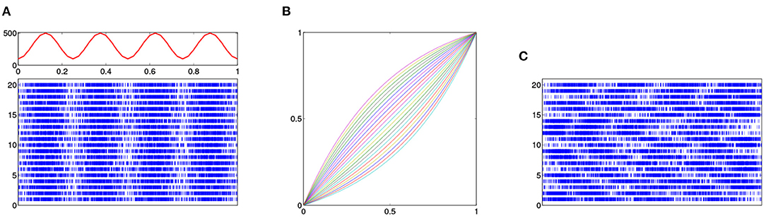
Figure 3. Simulation of Poisson process with compositional noise. (A) Intensity function of a Poisson process (top panel) and 20 independent realizations (bottom panel). (B) 20 time warping functions. (C) 20 observed processes, which are warped version of the original 20 realizations.

We then generate 20 warping functions ${\left\{{\gamma }_i\right\}}_{i=1}^{20}$ in the following form:

$\begin{array}{ll}{\gamma }_i(t)=\frac{e^{a_{i}t}-1}{e^{a_i}-1}.& (8)\end{array}$

Here a_i are equally spaced between −2 and 2, i = 1, ⋯ , 20. These warping functions are shown in Figure 3B. We then warp the 20 independent Poisson process using these 20 warping functions, respectively, by the formula in Equation (1). The resulting warped processes are shown in Figure 3C. Comparing these processes with those in Figure 3A, we can see that the positive relationship between number of events in each sub-region and the intensity value no longer exists. Given these noisy Poisson process observations, we aim to reconstruct the underlying intensity function λ(t).

The 20 true and estimated warped density functions are shown in the top and bottom panels, respectively, of Figure 4A. We can see that the kernel method provides a reasonable estimation for the warped intensity functions. The intensity function λ(t) is estimated for two different cases: (1) the time warping is ignored during estimation (i.e., naive method), and (2) the time warping is accounted for in the estimation using the proposed method. Both of these estimates are displayed with the true intensity function in Figure 4B by 3 different colors: true (black), proposed (blue), and naive (green). The naive estimated intensity underestimates the true intensity in the middle two-thirds of the curve and the true waveform pattern is not revealed. In contrast, the proposed method provides a much better estimate of the true intensity function. To compare with more methods, we also show estimation result using Fisher-Rao metric (cyan) [33] and Wasserstein distance (red) [32] in Figure 4B. For accuracy measurement, the 𝕃¹-, 𝕃²-, and 𝕃^∞- norms are adopted to measure the error in each estimation method and the reuslt is shown in Table 2. We can see that the proposed method has the smallest error regardless of which norm is used.

FIGURE 4

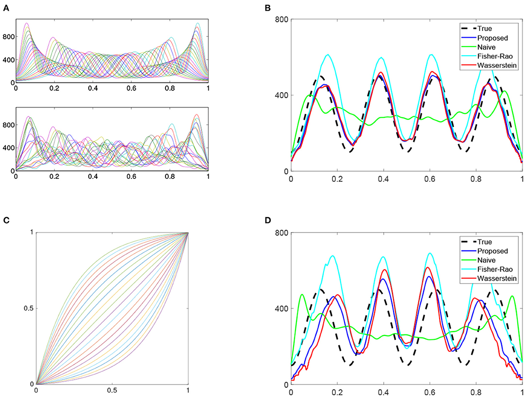
Figure 4. Intensity estimation. (A) Top panel: True warped density functions. Bottom panel: estimated individual density functions using warped processes in Figure 3C. (B) True and estimated intensity functions using four methods: proposed, naive, Fisher-Rao, and Wasserstein. (C) More drastic warping functions in the 2nd Simulation. (D) Same as (B) except for the 2nd simulation.

TABLE 2

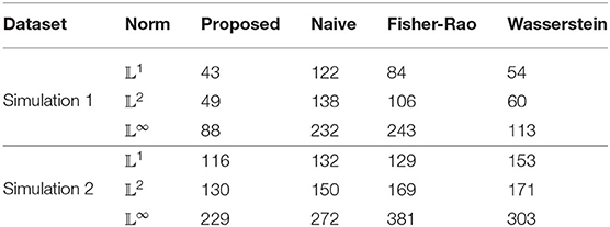
Table 2. Estimation errors for each method in two simulated datasets.

We can also test the estimation performance of each method when the warping functions are more drastic. Such functions can be simulated by letting a_i in Equation (8) be equally spaced between −4 and 4. These warping functions are shown in Figure 4C. In this 2nd simulation, the performance decreases in all methods (shown in Figure 4D and Table 2). However, the proposed method still has the lowest error by using each of the three norms.

3.2. Simulation 2: Poisson Process With a Non-negative Intensity Function

In this second example, we illustrate the estimation method for non-negative intensity functions in section 2.3. The underlying intensity function is defined on [0, 1] and given in the following form:

$\lambda (t)=\{\begin{array}{cc}-16000|t-0.5|+4000& t\in [0.25,0.75]\\ 0& \text{otherwise}\end{array}$

This intensity, shown in Figure 5A, has a triangular shape with peak at 0.5 and two flat sub-regions, [0, 0.25] and [0.75, 1].

FIGURE 5

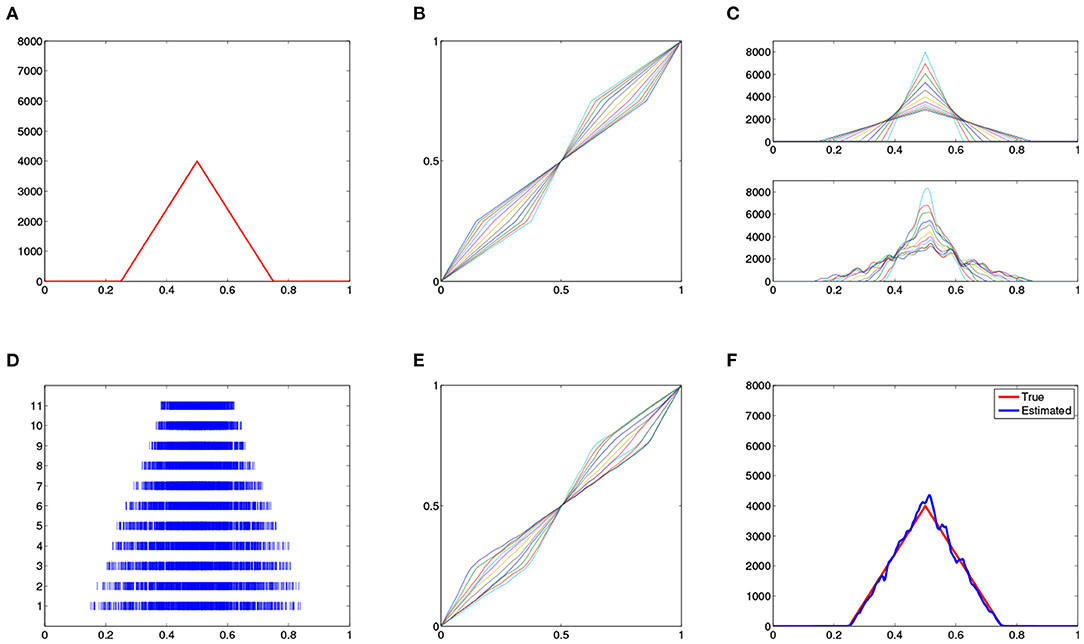
Figure 5. Non-negative intensity estimation. (A) True intensity function. (B) 11 warping functions. (C) (top panel) True warped intensity functions and (bottom panel) estimated intensities with modified kernel method. (D) 11 simulated processes with respect to the warped intensities. (E) Estimated warping functions. (F) Estimated (blue) and true (red) intensity functions.

We then generate 11 warping functions ${\left\{{\gamma }_i\right\}}_{i=1}^{11}$ in the following two steps: At first, we define ${\tilde{\gamma }}_i\in \Gamma$ on [0, 1] as:

$\begin{array}{ll}{\tilde{\gamma }}_i(t)=\frac{\text{sign}(2t-1)|2t-1{|}^{e_i}+1}{2}& (9)\end{array}$

where

$e_i=\{\begin{array}{cc}\frac{1}{2-0.2(i-1)}& i=1,\dots ,6\\ 0.2(i-6)+1& i=7,\dots ,11.\end{array}$

Then, each γ_i(t) is defined by linearizing ${\tilde{\gamma }}_i(t)$ at the value points t = [0, 0.25, 0.5, 0.75, 1]. These warping functions are shown in Figure 5B. The warped intensity functions, ${\lambda }_i(t)=\lambda ({\gamma }_i(t))\dot{\gamma }(t)$, are shown in the top panel of Figure 5C. We then simulate 11 independent Poisson processes using these 11 intensity functions, respectively, and the results are shown in Figure 5D. We can see that these realizations clearly display the warped intensity functions along the time axis. Given these noisy Poisson process observations, we aim to reconstruct the underlying intensity function λ(t).

We first estimate the warped intensity functions using modified kernel method on the 11 observed realizations. The result is shown in the lower panel of Figure 5C. Comparing with the true intensities in the upper panel, we can see the kernel method provides a reasonable estimation. In spite of the phase shift along the time axis, the kernel method estimates the flat subregions in the underlying intensity appropriately.

Once the individual intensities are estimated, we then compute their Karcher mean to get the the warping functions shown in Figure 5E. These warping functions are then used to estimate the underlying intensity function for the process and the result is shown in Figure 5F. Comparing the result with the true intensity function, we find that the proposed method provides a very accurate reconstruction.

3.3. Application in Spike Train Data

In this section the proposed intensity estimation method will be applied to a benchmark spike train dataset. This dataset was first used in a metric-based analysis of spike trains [14], and was also used as a common data set in a workshop on function registration, CTW: Statistics of Time Warpings and Phase Variations in Mathematical Bioscience Institute in 2012. It is publicly available from http://mbi.osu.edu/2012/stwdescription.html. In brief, the spiking activity of one neuron in primary motor cortex was recorded in a juvenile female macaque monkey. In the experimental setting, a subject monkey was trained to perform a closed Squared-Path (SP) task by moving a cursor to targets via contralateral arm movements in the horizontal plane. Basically, the targets in the SP task are all fixed at the four corners of a square and the movement is stereotyped. In each trial the subject reached a sequence of 5 targets which were the four corners of the square with the first and last targets overlapping. Each sequence of 5 targets defined a path, and there were four different paths in the SP task (depending on the starting point). In this experiment, 60 trials for each path were recorded, and the total number of trials was 240.

To fix a standardized time interval for all data, the spiking activity in each trial is normalized to 5 s. Thirty spike trains in each path are shown in Figure 6 where temporal variation across the trains can be clearly observed. For the purpose of intensity estimation, a truncated Gaussian kernel (width = 41.67 ms) is adopted to estimate the underlying density of each of the point process spike trains. From these data, we observe that the densities have a similar pattern within each class; for example, they have similar number of peaks and the locations of these peaks are only slightly different. Such difference can be treated as compositional noise within each path. We also note that the peak locations across different paths are significantly different.

FIGURE 6

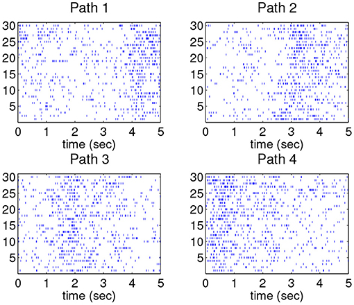
Figure 6. 30 spike trains in each of the four movement paths.

For the 60 trials in each path, the first 30 of them are chosen as the training data and the last 30 as the test data. The proposed intensity estimation method is tested here to decode neural signals with respect to different movement paths. Basically, we classify each smoothed test trial using the smallest value of the distances to the four Karcher means in four movement paths in the training set.

The underlying intensity function for each path is calculated using the proposed algorithm, and the result is shown in Figure 7. Comparing with the original spike trains, all of the mean spike trains appropriately represent the firing patterns in the corresponding movement. For example, the spiking frequency is relatively higher when the hand moves upward, which is apparent in all four means. For the 120 test trains, each train is labeled by the shortest distance over the distances to the four means in the training set. We only need to compute 120 × 4 = 480 distances. It is found that the classification accuracy using the proposed estimation method is 82.5%(99/120) whereas the classification accuracies using the naive cross-sectional method and the Fisher-Rao registration method are 77.5%(93/120) and 55.0%(66/120), respectively. This result shows the proposed method can better differentiate neural signals with respect to different movement behaviors.

FIGURE 7

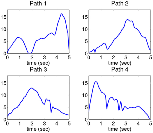
Figure 7. Estimated intensity function in each path.

4. Discussion

Intensity estimation has been a classical problem in Poisson process methods. The problem is significantly challenging if the observed data are corrupted with compositional noise, i.e., there is time warping noise in each realization. In the paper, we have proposed a novel alignment-based algorithm for positive intensity estimation. The method is based on a key fact that the intensity function is area-preserved with respect to compositional noise. Such a property implies that the time warping is only encoded in the normalized intensity, or density, function. Based on this finding, we decompose the estimation of intensity by the product of estimated total intensity and estimated density. Our investigation on asymptotics shows that the proposed estimation algorithm provides a consistent estimator for the underlying density. We further extend the method to all non-negative intensity functions, and provide simulation examples to illustrate the success of the estimation algorithms.

While results from this method show promising improvements over previous methods, it is important to note that the method is dependent upon the kernel density estimates of the observed processes. In general, kernel density estimates are highly dependent upon the chosen bandwidth h [38, 39]. In this paper, we have used a simple plug-in method to determine an appropriate bandwidth. In future work, we will consider the development of an algorithm that can automatically choose the optimal bandwidth for the modified kernel density estimator. Additionally, future work will examine the asymptotic variability of this estimator and an extension to general Cox processes for conditional intensity estimation.

Data Availability Statement

The data analyzed in this study is not publicly available. Requests to access these datasets should be directed to Wei Wu, at wwu@stat.fsu.edu.

Author Contributions

GS designed the proposed framework, conducted computational analysis, and wrote the paper. WW designed the proposed framework, supervised and conducted data analysis, and wrote the paper. AS supervised, data analysis, and wrote the paper. All authors contributed to the article and approved the submitted version.

Conflict of Interest

The authors declare that the research was conducted in the absence of any commercial or financial relationships that could be construed as a potential conflict of interest.

Publisher's Note

All claims expressed in this article are solely those of the authors and do not necessarily represent those of their affiliated organizations, or those of the publisher, the editors and the reviewers. Any product that may be evaluated in this article, or claim that may be made by its manufacturer, is not guaranteed or endorsed by the publisher.

Supplementary Material

The Supplementary Material for this article can be found online at: https://www.frontiersin.org/articles/10.3389/fams.2021.648984/full#supplementary-material

References

1. Chiang CT, Wang MC, Huang CY. Kernel estimation of rate function for recurrent event data. Scand Stat Theor Appl. (2005) 32:77–91. doi: 10.1111/j.1467-9469.2005.00416.xn

PubMed Abstract | CrossRef Full Text | Google Scholar

2. Kolaczyk ED. Wavelet shrinkage estimation of certain poisson intensity signals using corrected thresholds. Stat Sin. (1999) 9:119–35.

Google Scholar

3. Nowak RD, Timmermann KE. Stationary Wavelet-Based Intensity Models for Photon-Limited Imaging. IEEE (1998).

Google Scholar

4. Brown EN, Frank LM, Tang D, Quirk MC, Wilson MA. A statistical paradigm for neural spike train decoding applied to position prediction from ensemble firing patterns of rat hippocampal place cells. J Neurosci. (1998) 18:7411–25. doi: 10.1523/JNEUROSCI.18-18-07411.1998

PubMed Abstract | CrossRef Full Text | Google Scholar

5. Brockwell AE, Rojas AL, Kass RE. Recursive Bayesian decoding of motor cortical signals by particle filtering. J Neurophysiol. (2004) 91:1899–907. doi: 10.1152/jn.00438.2003

PubMed Abstract | CrossRef Full Text | Google Scholar

6. Lawlor PN, Perich MG, Miller LE, Kording KP. Linear-nonlinear-time-warp-poisson models of neural activity. J Comput Neurosci. (2018) 45:173–91. doi: 10.1007/s10827-018-0696-6

PubMed Abstract | CrossRef Full Text | Google Scholar

7. Donoho DL. Nonlinear Wavelet Methods for Recovery of Signals, Densities, and Spectra From Indirect and Noisy Data. Stanford University (1993). p. 437.

Google Scholar

8. Reynaud-Bouret P, Rivoirard V. Near optimal thresholding estimation of a Poisson intensity on the real line. Electron J Stat. (2010) 4:172–238. doi: 10.1214/08-EJS319

CrossRef Full Text | Google Scholar

9. Bartoszynski R, Brown BW, McBride CM, Thompson JR. Some nonparametric techniques for estimating the intensity function of a cancer related nonstationary poisson process. Ann Stat. (1981) 9:1050–60. doi: 10.1214/aos/1176345584

CrossRef Full Text | Google Scholar

10. Diggle P. A kernel method for smoothing point process data. J Appl Stat. (1985) 34:138–47. doi: 10.2307/2347366

CrossRef Full Text | Google Scholar

11. Arjas E, Gasbarra D. Nonparametric Bayesian inference from right censored survival data, using the Gibbs Sampler. Stat Sin. (1994) 4:505–24.

Google Scholar

12. Guida M, Calabria R, Pulcini G. Bayes inference for a non-homogeneous Poisson process with power intensity law. IEEE Trans. Reliabil. (1989) 38:603–9. doi: 10.1109/24.46489

CrossRef Full Text | Google Scholar

13. Timmermann KE, Nowak RD. Multiscale Bayesian Estimation of Poisson Intensities. (1997).

Google Scholar

14. Wu W, Srivastava A. An information-geometric framework for statistical inferences in the neural spike train space. J Comput Neurosci. (2011) 31:725–48. doi: 10.1007/s10827-011-0336-x

PubMed Abstract | CrossRef Full Text | Google Scholar

15. Ramsay JO, Li X. Curve registration. J R Stat Soc Ser B. (1998) 60:351–63. doi: 10.1111/1467-9868.00129

CrossRef Full Text | Google Scholar

16. Gervini D, Gasser T. Self-modeling warping functions. J R Stat Soc Ser B. (2004) 66:959–71. doi: 10.1111/j.1467-9868.2004.B5582.x

CrossRef Full Text | Google Scholar

17. Tang R, Muller HG. Pairwise curve synchronization for functional data. Biometrika. (2008) 95:875–89. doi: 10.1093/biomet/asn047

CrossRef Full Text | Google Scholar

18. James G. Curve alignments by moments. Ann Appl Stat. (2007) 1:480–501. doi: 10.1214/07-AOAS127

CrossRef Full Text | Google Scholar

19. Tucker JD, Wu W, Srivastava A. Generative models for functional data using phase and amplitude separation. Comput Stat Data Anal. (2013) 61:50–66. doi: 10.1016/j.csda.2012.12.001

CrossRef Full Text | Google Scholar

20. Bigot J, Gadat S, Klein T, Marteau C. Intensity estimation of non-homogeneous poisson processes from shifted trajectories. Electron J Stat. (2013) 7:881–931. doi: 10.1214/13-EJS794

CrossRef Full Text | Google Scholar

21. Panaretos VM, Zemel Y. Amplitude and phase variation of point processes. Ann Stat. (2016) 44:771–812. doi: 10.1214/15-AOS1387

CrossRef Full Text | Google Scholar

22. Ross SM. Introduction to Probability Models. Elsevier (2010).

Google Scholar

23. Kurtek S, Srivastava A, Wu W. Signal estimation under random time-warpings and nonlinear signal alignment. In: Proceedings of Neural Information Processing Systems (NIPS). (2011).

Google Scholar

24. Ramsay JO. Estimating smooth monotone functions. J R Stat Soc Ser B Stat Methodol. (1998) 60:365–75. doi: 10.1111/1467-9868.00130

CrossRef Full Text | Google Scholar

25. Kneip A, Li X, Ramsay JO. Curve registration by local regression. Can J Stat. (2000) 28:19–29. doi: 10.2307/3315251.n

CrossRef Full Text | Google Scholar

26. Kneip A, Ramsay JO. Combining registration and fitting for functional models. J Am Stat Assoc. (2008) 103:1155–65. doi: 10.1198/016214508000000517

CrossRef Full Text | Google Scholar

27. Srivastava A, Wu W, Kurtek S, Klassen E, Marron JS. Registration of functional data using Fisher-Rao metric. arXiv preprint. arXiv:1103.3817v2 (2011).

Google Scholar

28. Reynaud-Bouret P. Adaptive estimation of the intensity of inhomogeneous Poisson processes via concentration inequalities. Probabil Theor Relat Fields. (2003) 126:103–53. doi: 10.1007/s00440-003-0259-1

CrossRef Full Text | Google Scholar

29. Willett RM, Nowak RD. Multiscale Poisson intensity and density estimation. IEEE Trans Inform Theor. (2007) 53:3171–87. doi: 10.1109/TIT.2007.903139

CrossRef Full Text | Google Scholar

30. Bhattacharyya A. On a measure of divergence between two statistical populations defined by their probability distributions. Bull Calcutta Math Soc. (1943) 35:99–109. doi: 10.1515/crll.1909.136.210

CrossRef Full Text | Google Scholar

31. Hellinger E. Neue Begründung der Theorie quadratischer Formen von unendlichvielen Veränderlichen. J Reine Angew Math. (1909) 136:210–71.

32. Wasserstein LN. Markov processes over denumerable products of spaces describing large systems of automata. Probl Inform Transm. (1969) 5:47–52.

Google Scholar

33. Srivastava A, Jermyn I, Joshi SH. Riemannian analysis of probability density functions with applications in vision. In: IEEE Conference on Computer Vision and Pattern Recognition. (2007). p. 1–8.

Google Scholar

34. Cline DBH, Hart JD. Kernel estimation of densities of discontinuous derivatives. Statistics. (1991) 22:69–84. doi: 10.1080/02331889108802286

CrossRef Full Text

35. Schuster EF. Incorporating support constraints into nonparametric estimators of densities. Commun Stat Part A Theor Methods. (1985) 14:1123–36. doi: 10.1080/03610928508828965

CrossRef Full Text | Google Scholar

36. Silverman BW. Density Estimation for Statistics and Data Analysis. Chapman and Hall/CRC (1986).

Google Scholar

37. Wu W, Srivastava A. Estimation of a mean template from spike-train data. Conf Proc IEEE Eng Med Biol Soc. (2012) 2012:1323–6. doi: 10.1109/EMBC.2012.6346181

PubMed Abstract | CrossRef Full Text | Google Scholar

38. Ramsay JO, Silverman BW. Functional Data Analysis, 2nd Edn. New York, NY: Springer Series in Statistics (2005).

Google Scholar

39. Ferraty F, Vieu P. Nonparametric Functional Data Analysis, Theory and Practice. Springer Series in Statistics (2006).

Google Scholar