Physics-Aware Deep-Learning-Based Proxy Reservoir Simulation Model Equipped With State and Well Output Prediction

1 Introduction

In this study, we build upon a recent study on embedding physical constraints to machine learning architectures to efficiently and accurately solve large-scale reservoir simulation problems [1, 2]. Scientific Machine Learning (SciML) is a rapidly developing area in reservoir simulation. SciML introduces regularizing physics constraints, allowing predicting future performance of complex multiscale, multiphysics systems using sparse, low-fidelity, and heterogeneous data. Here, we address the problem of creating consistent input–output relations for a reservoir run, taking into account physical constraints such as mass conservation, multiphase flow flux matching, and well outputs (rates) derived directly from data.

Simulation of complex problems can usually be performed by recasting the underlying partial differential equations into a (non-linear) dynamical system state-space representation. This approach has been explored in numerical petroleum reservoir simulation, and several techniques were developed or applied to handle the intrinsic nonlinearities of this problem [3]. The main idea is to extract information from states, which are usually given by phase pressures and saturations—as in multiphase flow in porous media with no coupling with additional phenomena, such as geomechanics. Although state-space models can be easily manipulated, the transformation of the reservoir simulation equations induces systems with a very large number of states. In this case, model reduction methods [4, 5] can be used to reduce the complexity of the problem and mitigate the large computation cost associate with the solution under consideration.

The area of model order reduction (MOR) for reservoir simulation has been very active in the past decade and goes beyond recent projection-based MOR developments. Methods such as upscaling, proxy and surrogate modeling, and parameterization have always found their ways in reservoir simulation. It is not the intention here to give a comprehensive historical account of MOR, but two methods have emerged as good candidates for projection-based MOR: POD-TPWL [5–7] and POD-DEIM [8–10]. Each of these methods has its advantages and drawbacks, which have been discussed in many published articles [9, 11]. The unifying framework in these methods is projection; that is, we project the original large state-space model into a much smaller space of (almost) non-physical significance. The recovery of physical meaning is usually attained by proper training and storage of the states of the system. Although very efficient algorithms can be used for improving state selection through clustering and adaptation, the lack of physical meaning can hinder the application of complex phenomena simulations. This is to say that the reduced-order model’s output, that is, well rates and bottom-hole pressures, can sometimes differ significantly from the original fine-scale simulation.

Data-driven modeling in reservoir engineering is not new [12]. Many data-analytics and statistical multi-variable regression have been applied in reservoir simulation to obtain fast proxy models [13, 14]. Recently there has been an explosion of methods associated at large with machine learning algorithms [15–17]. It is our view, however, that the machinery developed with physics-based model reduction, especially the strategies derived from state-space identification, can be enhanced with machine learning algorithms. System identification can lead to parametric models where the structure of the model is predefined (see Figure 1, for instance, for the state-space representation), whereas machine learning methods lead to non-parametric models and depend largely on the number of training points [18, 19].

FIGURE 1

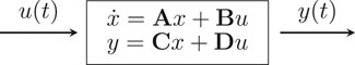
FIGURE 1. System representation.

A combination of data-driven model reduction strategies and machine learning (deep-neural networks–DNN) will be used here to achieve state and input–output matching simultaneously. In [2], the authors use a DNN architecture to predict the state variables evolution after training an autoencoder coupled with a control system approach (Embed to Control—E2C) and adding some physical components (Loss functions) to the neural network training procedure. The idea was to use the framework of the POD-TPWL as a way to recast the reservoir simulator from a system perspective and obtain reduced-order states out of the encoding blocks. Physical constraints were handled by employing particular loss functions related to mass conservation.

In this study, we extend this idea by adding the simulation model output, for example, well bottom-hole pressure and well flow rates, as data to be used in the training procedure. The contributions here are twofold: first, we have extended the E2C to the E2CO (E2C and Observe) form, which allows a generalization of the method to any type of well model. By doing this, it is possible to estimate the evolution in time of both the state variables as well as the output variables simultaneously. Second, our new formulation provides a fast and reliable proxy for the simulation outputs that can be coupled with other components in reservoir management workflows—for instance, well-control optimization workflows such a non-intrusive method, like data-driven models, does not need to have access to reservoir simulation internal structure so that it can be easily applied to commercial reservoir simulations. We view this as an analogous step to system identification whereby mappings related to state dynamics, inputs (controls), and measurements (output) are obtained.

This study is organized as follows. We start by giving a brief overview of numerical reservoir simulation, focusing on the aspects that will be used to develop the ideas presented here, such as identifying states. Next, we revisit the model order reduction (MOR) framework and the methods used here, such as the trajectory piecewise linearization—TPWL and proper orthogonal decomposition—POD. Then, we describe the machine learning architecture E2C and revisit the methodology used as a basis for our study. This leads to the introduction of our main contribution and new propositions to handle the reservoir outputs. Finally, we give details of our implementation and a description of the training set’s data. We show the results comparing the propositions, and we draw some conclusions in the end.

1.1 Numerical Petroleum Reservoir Simulation

Widely used in all phases of development of an oil field, reservoir simulations are applied to model flow dynamics and predict reservoir performance from preliminary exploration until the full development stage of petroleum production. A deep understanding of the model, discretization, and solution methods can be found in [20, 21].

A reservoir simulator is a combination of rock and geological structure properties, fluid properties, and a mathematical representation of the subsurface flow dynamics. A two-phase (oil and water) two-dimensional reservoir simulator is based on flow equations represented in Eq. 1.

$\nabla \left[\overrightarrow{\overrightarrow{k}}\frac{k_{r,j}\left(S_j\right)}{{\mu }_j}{\rho }_j\nabla P_j\right]+q_j-\frac{\partial }{\partial t}\left(\varphi S_j{\rho }_j\right)=0,(1)$

where the subscript j represents the phase oil or water, k is the absolute permeability, $k_r$ is the relative permeability, µ is the viscosity, ρ is the fluid density, and ϕ is porosity. The solution we seek here is $P_j,S_j$.

It is possible to identify three terms on Eq. 1: the first one is the flux term, followed by the source/sink term, and the last one is the accumulation term. Although we only describe a two-phase flow system, these equations can easily generalize for multiphase flow simulations. As stated before, the reservoir simulation equations can be recast in a systems framework, where the nonlinear equations can be linearized into a time-varying state-space model as depicted in Figure 1. Note that while the controls u are imposed on the wells, the state x evolution is calculated based on the discretized partial differential equation (Eq. 1), and the output y is observed on the wells.

In general, the wells can be controlled by flow rates or bottom-hole pressure (BHP). Here we will assume that the producer wells are controlled by BHP and injector wells are controlled by injection rate ($q_{inj}$). So, we can define a control vector composed of the controls for all wells at a timestep t as:

$u^t=\left[\begin{array}{c}{\text{BHP}}^t\\ q_{\text{inj}}^t\end{array}\right],$

where ${\text{BHP}}^t={\left[\begin{array}{ccc}{\text{BHP}}_1^t& \dots & {\text{BHP}}_p^t\end{array}\right]}^T$, $q_{\text{inj}}^t={\left[\begin{array}{ccc}{q}_{\text{inj},1}^t& \dots & q_{\text{inj},i}^t\end{array}\right]}^T$, p is the number of producers, and i the number of injectors.

The state dynamical evolution will be solved for each timestep t. The state is represented as:

$x^t=\left[\begin{array}{c}{P}^t\\ S^t\end{array}\right],$

where $P^t={\left[\begin{array}{ccc}{P}_1^t& \dots & P_n^t\end{array}\right]}^T$, $S^t={\left[\begin{array}{ccc}{S}_1^t& \dots & S_n^t\end{array}\right]}^T$, and n is the number of gridblocks.

The output for the producers is the oil flow rate ($q_o$) and the water flow rate ($q_w$) and for the injectors is the bottom hole pressure (BHP). Thus, the output vector can be defined as:

$y^t=\left[\begin{array}{c}{q}_o^t\\ q_w^t\\ {\text{BHP}}^t\end{array}\right],(2)$

where $q_o^t={\left[\begin{array}{ccc}{q}_{o,1}^t& \dots & q_{o,p}^t\end{array}\right]}^T$, $q_w^t={\left[\begin{array}{ccc}{q}_{w,1}^t& \dots & q_{w,p}^t\end{array}\right]}^T$, ${\text{BHP}}^t={\left[\begin{array}{ccc}{\text{BHP}}_1^t& \dots & {\text{BHP}}_i^t\end{array}\right]}^T$. These values are calculated using the Peaceman equation [22]. For example, for a producer well, the flow rate of phase j can be calculated as:

$q_j=\frac{k_{r,j}}{B_j{\mu }_j}\text{WI}\left(P_j-BHP\right),(3)$

where WI is the well index and can be calculated as:

$\text{WI}=\frac{2\pi \alpha kh}{\text{ln}\left(\frac{r_o}{r_w}\right)+\text{SKIN}},$

where α is a unit conversion factor, h is the height of the reservoir gridblock, $r_o$ is the grid block dimension equivalent radius, $r_w$ is the wellbore radius, and SKIN is the skin factor.

Following the assumptions as in [3] and the application of fully implicit discretization it is possible to write the residual form of Eq. 1 as:

$g\left(x^{t+1},u^{t+1}\right)=\mathbf{F}\left(x^{t+1}\right)+\mathbf{Acc}\left(x^{t+1},x^t\right)+\mathbf{Q}\left(x^{t+1},u^{t+1}\right)=0,(4)$

where we can identify the flux term $\mathbf{F}\left(x^{t+1}\right)$, the accumulation term $\mathbf{Acc}\left(x^{t+1},x^t\right)$, and the source and sink term $\mathbf{Q}\left(x^{t+1},u^{t+1}\right)$.

This equation can be solved by the Newton’s method by defining the Jacobian matrix $\mathbf{J}=\frac{\partial g}{\partial x}$. So, the state evolution can be calculated as:

$x^{t+1}=x^t-{\left({\mathbf{J}}^{t+1}\right)}^{-1}\left[\mathbf{F}\left(x^{t+1}\right)+\mathbf{Acc}\left(x^{t+1},x^t\right)+\mathbf{Q}\left(x^{t+1},u^{t+1}\right)\right].(5)$

To apply reduced-order modeling techniques to reservoir simulation efficiently, one can linearize the residual Eq. 4 (or Eq. 5). In Ref. [23], the authors presented the linearization for a single-phase 2D reservoir based on the simulator’s Jacobian matrix. Van Doren et al. [24] and Heijn et al. [25] developed similar approaches for a two-phase reservoir. These linearization methods were developed aligned to a control system approach, and the reader can find a comprehensive review of the control system applied to reservoir simulation in [3]. Committing with the control system approach, a state-space representation of a linear system can be written as Eq. 6. The authors cited in this paragraph manipulated equations similar to Eq. 4 or Eq. 5 to linearize them and write as a linear system.

$\{\begin{array}{c}\dot{x}={\mathbf{A}}_{c}x+{\mathbf{B}}_{c}u\\ y={\mathbf{C}}_{c}x+{\mathbf{D}}_{c}u\end{array},(6)$

where x represents the state, $\dot{x}$ the state time derivative ($\frac{\text{d}x}{\text{d}t}$), and u the inputs (controls) and y the system output. ${\mathbf{A}}_c$ is called state matrix, ${\mathbf{B}}_c$ input matrix, ${\mathbf{C}}_c$ output matrix, and ${\mathbf{D}}_c$ is the feed-through matrix. The subscript c stands for continuous time. It is worth mentioning that on Eq. 6 we are presenting the state evolution equation (first one) and the output equation (second one), but the focus of linearization method is to be applied on the state evolution equation.

In general, it is necessary to choose a linearization point in time and use the Jacobian matrix at this time to calculate previously presented matrices. If the system dynamic strongly changes over time, the choice of a fixed linearization time can lead to large estimation errors. Techniques like TPWL (trajectory piecewise linearization) have been used to overcome these difficulties, where it is possible to approximate matrices $\mathbf{A}$, $\mathbf{B}$, $\mathbf{C}$, and $\mathbf{D}$ at each interest time.

In the next section, we will present the linearization method TPWL that, combined with a model order reduction technique called proper orthogonal decomposition (POD), has been successfully applied to reservoir simulation [6].

1.2 Trajectory Piecewise Linearization (TPWL)

Trajectory piecewise linearization is a method composed of two main steps. The first step is a training procedure (offline processing) that aims to capture state snapshots of a high-fidelity solution for the system to be linearized. These state snapshots are stored along with the Jacobian matrix of each timestep.

The purpose of the second step (online processing) is to predict the state on the next timestep $x^{t+1}$ based on the current state $x^t$ and the control state $u^t$. The idea here is to use the stored states on the training step in order to predict the new state. First, in the group of the stored state snapshots, we identified the snapshot $x^i$ closest to $x^t$. Then, we use the stored state and the Jacobian matrix for i and $i+1$ to calculate the state $x^{t+1}$ using the following equation:

$x^{t+1}=x^{i+1}-{\left({\mathbf{J}}^{i+1}\right)}^{-1}\left[{\mathbf{F}}^{i+1}+\mathbf{Ac}{\mathbf{c}}^{i+1}+\frac{\partial \mathbf{Ac}{\mathbf{c}}^{i+1}}{\partial x^i}\left(x^t-x^i\right)+\mathbf{Q}\left(x^{i+1},u^{t+1}\right)\right].(7)$

Previously, we wrote the state evolution equation of the reservoir simulation solution (Eq. 5) as a linearized system (Eq. 6). Using similar approach, we can rewrite the TPWL equation (Eq. 7) as a linearized system:

$\{\begin{array}{c}{x}^{t+1}={\mathbf{A}}^i{x}^t+{\mathbf{B}}^i{u}^t\\ y^{t+1}={\mathbf{C}}^i{x}^{t+1}+{\mathbf{D}}^i{u}^t\end{array},(8)$

where $\mathbf{A}$, $\mathbf{B}$, $\mathbf{C}$, and $\mathbf{D}$ are the time discretized version of the continuous matrices, and the superscript i represents the linearized matrices using information from the snapshot i.

To solve Eq. 7 and to compute matrices ${\mathbf{A}}^i$, ${\mathbf{B}}^i$, ${\mathbf{C}}^i$, and ${\mathbf{D}}^i$ it is necessary to calculate the inverse of the Jacobian matrix , which is computationally costly. Furthermore, storing a full state and a full Jacobian matrix for each timestep on the training runs requires a huge memory amount. The next section will show how to use a model order reduced method to solve these problems.

1.3 Proper Orthogonal Decomposition (POD)

The states stored on the training step of the TPWL can be arranged on:

$\mathbf{X}=\left[\begin{array}{cccc}{x}^1& x^2& \dots & x^n\end{array}\right].$

It is possible to take the singular value decomposition (SVD) of $\mathbf{X}$. Based on some criteria, one can choose to keep only the l largest singular values. The POD basis $\text{Φ}$ is defined as the l right singular vectors, and the reduced/latent state space z is then defined as a projection of the original space x based on the POD basis:

$z={\text{Φ}}^{T}x.(9)$

Using the relation $x\approx \text{Φ}z$ we can rewrite Eq. 7 as:

${\mathbf{J}}^{i+1}\text{Φ}\left(z^{t+1}-z^{i+1}\right)=-\left[{\mathbf{F}}^{i+1}+\mathbf{Ac}{\mathbf{c}}^{i+1}+\frac{\partial \mathbf{Ac}{\mathbf{c}}^{i+1}}{\partial x^i}\text{Φ}\left(z^t-z^i\right)+\mathbf{Q}\left(x^{i+1},u^{t+1}\right)\right],(10)$

and multiplying both sides of the above equation by ${\text{Φ}}^T$:

${\text{Φ}}^T{\mathbf{J}}^{i+1}\text{Φ}\left(z^{t+1}-z^{i+1}\right)=-{\text{Φ}}^T\left[{\mathbf{F}}^{i+1}+\mathbf{Ac}{\mathbf{c}}^{i+1}+\frac{\partial \mathbf{Ac}{\mathbf{c}}^{i+1}}{\partial x^i}\text{Φ}\left(z^t-z^i\right)+\mathbf{Q}\left(x^{i+1},u^{t+1}\right)\right].(11)$

Now, defining the reduced Jacobian matrix as ${\mathbf{J}}_r^{i+1}={\text{Φ}}^T{\mathbf{J}}^{i+1}\text{Φ}$ and the other reduced terms as ${\mathbf{F}}_r^{i+1}={\text{Φ}}^T{\mathbf{F}}^{i+1}$, $\mathbf{Ac}{\mathbf{c}}_r^{i+1}={\text{Φ}}^T\mathbf{Ac}{\mathbf{c}}^{i+1}$, ${\left(\partial \mathbf{Ac}{\mathbf{c}}^{i+1}/\partial x^i\right)}_r={\text{Φ}}^T\left(\partial \mathbf{Ac}{\mathbf{c}}^{i+1}/\partial x^i\right)\text{Φ}$, and ${\mathbf{Q}}_r={\text{Φ}}^T\mathbf{Q}$, we can rewrite Eq. 11 as the POD-TPWL equation:

$z^{t+1}=z^{i+1}-{\left({\mathbf{J}}_r^{i+1}\right)}^{-1}\left[{\mathbf{F}}_r^{i+1}+\mathbf{Ac}{\mathbf{c}}_r^{i+1}+{\left(\frac{\partial \mathbf{Ac}{\mathbf{c}}^{i+1}}{\partial x^i}\right)}_r\left(z^t-z^i\right)+{\mathbf{Q}}_r\left(x^{i+1},u^{t+1}\right)\right].(12)$

By truncating the latent space, we deal with smaller dimension matrices when compared with the TPWL equation presented previously.

One can rewrite Eq. 12 as a linear time variant system:

$\{\begin{array}{c}{z}^{t+1}={\mathbf{A}}_r^i{z}^t+{\mathbf{B}}_r^i{u}^t\\ y^{t+1}={\mathbf{C}}_r^i{z}^{t+1}+{\mathbf{D}}_r^i{u}^t\end{array},(13)$

where ${\mathbf{A}}_r^i$, ${\mathbf{B}}_r^i$, ${\mathbf{C}}_r^i$, and ${\mathbf{D}}_r^i$ are the reduced version of the ones presented on Eq. 8.

The complexity of calculating matrices ${\mathbf{A}}_r^i$, ${\mathbf{B}}_r^i$, ${\mathbf{C}}_r^i$, and ${\mathbf{D}}_r^i$ (or its equivalents on Eqs. 6 and 8) can increase in more realistic cases (black-oil or compositional simulators). Another drawback of these methods is the mandatory access to the reservoir simulator code to extract the Jacobian matrix and other data structures from the simulator, which may turn impractical the use of these methods with commercial reservoir simulators.

In [1], the authors develop a method to calculate matrices ${\mathbf{A}}_r^t$ and ${\mathbf{B}}_r^t$ based on deep learning, using state snapshots as training data. Ref. [2] extended this idea by adding a physical loss function related to reservoir simulation. Here we expand on this and demonstrate the feasibility of extracting not only states but outputs.

2 Methods

In this section, we built upon a previously developed alternative to predict the state time evolution applied to numerical petroleum reservoir simulation based on deep learning, where a direct semi-empirical relation between the state and the output was used to calculate the well data. We will propose an improvement of well data estimation, first, by considering this data on the training process, and second, by building a specific network to estimate the output from the latent space that does not rely on the direct relation between the full state and the output.

2.1 Embed to Control (E2C)

This method was proposed in [1] for model learning and control of a nonlinear dynamical system using raw pixel images as input. It uses a convolutional autoencoder coupled with a control linear system approach to predict the time evolution of the system state.

In Figure 2, we present a schematic diagram showing the main elements for training this model. The inputs used on the training procedure are the elements shaded in gray ($x^t$, $x^{t+1}$, $u^t$, and $\text{Δ}{t}^t$). The variables with a hat ($\widehat{\cdot }$) are the estimated values. The paths presented with continuous arrows are used in both training and prediction steps, and those with dashed arrows are only used on the training procedures.

FIGURE 2

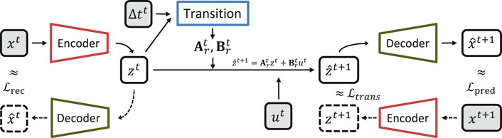
FIGURE 2. Diagram for training the E2C—Embed to control model.

The autoencoder is composed of an encoder that aims to transform the state in the original dimension space ($x^t$) to a reduced (latent) space ($z^t$), and a decoder that works as an inverted encoder to project back the reduced space state to the original space. One can relate the encoder with the POD projection (Eq. 9) since both have the ability to transform the original state x on the latent space state z.

The transition element uses the state in latent space to generate the matrices ${\mathbf{A}}_r^t$ and ${\mathbf{B}}_r^t$. These matrices are used to handle the dynamical system evolution using a linear control system approach, as in Eq. 14. Since this equation operates on the latent space, we can relate ${\mathbf{A}}_r^t$ and ${\mathbf{B}}_r^t$ with their reduced version used on Eq. 13.

${\widehat{z}}^{t+1}={\mathbf{A}}_r^t{z}^t+{\mathbf{B}}_r^t{u}^t.(14)$

It should be pointed out that matrices ${\mathbf{A}}_r^t$ and ${\mathbf{B}}_r^t$ change for each different input state $x^t$, like in other linearization procedures applied to reduced-order models techniques (e.g., TPWL—trajectory piecewise linearization).

Other important elements on this method are the 3 loss functions ($\mathrm{ℒ}$) that will be used during the training procedure. The reconstruction loss function ${\mathrm{ℒ}}_{\text{rec}}$ is introduced to guarantee the autoencoder (encoder and decoder) capability to reconstruct ${\widehat{x}}^t$ as close as possible to $x^t$. ${\widehat{x}}^t$ is calculated using:

${\widehat{x}}^t=\text{Decoder}\left(\text{Encoder}\left(x^t\right)\right).(15)$

The reconstruction loss function is defined as:

${\left({\mathrm{ℒ}}_{\text{rec}}\right)}_i={\left\{{\Vert x^t-{\widehat{x}}^t\Vert }_2^2\right\}}_i,(16)$

where i represents the sample index.

Minimizing the prediction loss guarantees the accuracy of the time evolution of the dynamical system. In this case, we define the prediction loss function as:

${\widehat{x}}^{t+1}=\text{Decoder}\left(\text{Transition}\left(\text{Encoder}\left(x^t\right)\right)\right),(17)$

where, ${\widehat{x}}^{t+1}$ is the prediction of the state variables at $t+1$, and then is possible to calculate the prediction loss:

${\left({\mathrm{ℒ}}_{\text{pred}}\right)}_i={\left\{{\left|\left|x^{t+1}-{\widehat{x}}^{t+1}\right|\right|}_2^2\right\}}_i.(18)$

The third loss function of the E2C model is the transition loss function, which tries to guarantee the model competence to evolve the reduced state z in time. This mimics the MOR idea of developing a projection framework in which the reduced state can evolve in time based on the reduced Jacobian matrix. First, we need to calculate:

${\widehat{z}}^{t+1}=\text{Transition}\left(\text{Encoder}\left(x^t\right)\right),$

and then:

$z^{t+1}=\text{Encoder}\left(x^{t+1}\right),$

and with these two equations it is possible to calculate the transition loss (Eq. 19):

${\left({\mathrm{ℒ}}_{\text{trans}}\right)}_i={\left\{{\Vert z^{t+1}-{\widehat{z}}^{t+1}\Vert }_2^2\right\}}_i.(19)$

Here, we briefly described the main elements of the E2C model. In the next section, we will show an improvement of this model, adding a physical loss function specifically designed to reservoir simulation problems.

2.2 Embed to Control with Physical Loss Function for Petroleum Reservoir Numerical Simulation

Inspired by the E2C model, Jin et al. [2] proposed an improvement on this model by adding a physical loss function to it. The model proposed by them focuses on the problem of building a proxy for a petroleum numerical reservoir simulator to be used on a well control optimization process. In Eq. 28 of [2], the authors introduced a physical loss function, reproduced below:

$\begin{array}{c}{\left({\mathrm{ℒ}}_p\right)}_i={\left\{{\Vert k\cdot \left[{\left(\nabla p^t-\nabla {\widehat{p}}^t\right)}_{\text{recon}}+{\left(\nabla p^{t+1}-\nabla {\widehat{p}}^{t+1}\right)}_{\text{pred}}\right]\Vert }_2^2\right\}}_i+\\ +\gamma {\left\{\Vert {\left(q^{w,t}-{\widehat{q}}^{w,t}\right)}_{\text{recon}}+{\left(q^{w,t+1}-{\widehat{q}}^{w,t+1}\right)}_{\text{recon}}\Vert \right\}}_i.\end{array}(20)$

This physical loss function is composed of two parts. The first one contains the mismatch between the predicted pressure gradient between adjacent grid blocks and the input pressure gradient multiplied by the permeability. This part of the proposed loss function intends to assure that the fluid flow between adjacent grid blocks in the predicted model is as close as possible to the input/true model. Simply put, this is basically a mass conservative requirement. Here, this first part of the physical loss function will be named the flux loss function.

The second part of the physical loss function deals with a mismatch in the producer wells’ flow rate. In fact, as described by the authors, it tries to guarantee that the producers’ grid block pressure in the predicted and reconstructed states are as close as possible to its equivalent on the input/true model. Instead of adding physics to the neural network, this second part adds more weight to the producers’ grid block pressure during the training procedure. In fact the authors in [2] did not use the flow rate on their physical loss function; instead, they used only the producers’ well grid block pressure. Since we will propose a new way to handle well data, we will omit this second part of the study’s proposed physical loss function. Even though we are omitting this part of the physical loss function, we will have it in our implementation of the method proposed by [2], for comparison purposes. Our implementation of their loss function (Eq. 28 of [2]) is presented here on Eq. 35.

We present in Figure 3 a diagram of the autoencoder with the flux loss function terms calculation. Comparing this figure with Figure 2, it is possible to notice the addition of the gradient calculation on both sides of the chart and also the calculation of the flux loss functions both in the reconstruction and prediction parts, which can be expressed as:

${\left({\mathrm{ℒ}}_{\text{flux},\text{rec}}\right)}_i=k{\left\{{\Vert \nabla p^t-\nabla {\widehat{p}}^t\Vert }_2^2\right\}}_i,(21)$

and

${\left({\mathrm{ℒ}}_{\text{flux},\text{pred}}\right)}_i=k{\left\{{\Vert \nabla p^{t+1}-\nabla {\widehat{p}}^{t+1}\Vert }_2^2\right\}}_i,(22)$

where k is the permeability.

FIGURE 3

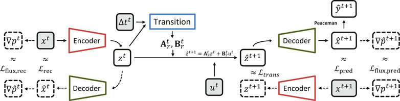
FIGURE 3. Diagram for training the E2C with flux loss.

The flux loss function can be defined as:

${\left({\mathrm{ℒ}}_{\text{flux}}\right)}_i={\left({\mathrm{ℒ}}_{\text{flux},\text{rec}}\right)}_i+{\left({\mathrm{ℒ}}_{\text{flux},\text{pred}}\right)}_i.(23)$

In addition to the flux loss function, on the top right of Figure 3, it is possible to see the calculation of the output ${\widehat{y}}_{t+1}$. The model outputs are well bottom hole pressure for the injector wells, and water and oil flow rates for the producer wells, in the case presented here. The calculation of these quantities from the state variables (pressures and saturations) is made by applying the Peaceman equation ([22]). This way to estimate the well data is here denoted by proposition 1. Note, that this is the actual proposed method in [2], implemented here for comparison purposes. In the following sections, we will propose and compare two other ways of estimating well data using E2C like models.

2.3 Embed to Control with Well Data Loss Functions for Petroleum Reservoir Numerical Simulation

Since we are building a proxy model for a petroleum reservoir numerical simulator to be applied in a well control optimization framework, we would like to emphasize the well data prediction (BHP and flow rates), not only on the state (pressure and saturation) calculation; or, in other words, we want to reconstruct the output and not only the states. To achieve this, we propose a well data loss function named ${\mathrm{ℒ}}_{\text{well}\_\text{data}2}$ as a reference to proposition 2. We present the diagram for proposition 2 in Figure 4, where it is possible to see the addition of the well data loss function on the right upper corner. This loss function will make the well data predicted by the model ${\widehat{y}}^{t+1}$ as close as possible to the true value $y^{t+1}$. Note that both y and $\widehat{y}$ are composed by oil and water flow rates and bottom hole pressures, as defined in Eq. 2. The input used to train the model is the well data calculated by a reservoir simulation. Proposition 2 well data loss function is defined as:

${\left({\mathrm{ℒ}}_{\text{well}\_\text{data}2}\right)}_i={\left\{{\Vert y^{t+1}-{\widehat{y}}^{t+1}\Vert }_2^2\right\}}_i.(24)$

To get a more reliable state prediction and, as consequence, a better well data estimation, we introduce a two-phase flux loss function (Eq. 25) for a two-phase simulator.

${\left({\mathrm{ℒ}}_{\text{flux}2\text{Ph}}\right)}_i={\left({\mathrm{ℒ}}_{\text{flux}2\text{Ph},\text{rec}}\right)}_i+{\left({\mathrm{ℒ}}_{\text{flux}2\text{Ph},\text{pred}}\right)}_i,(25)$

where its terms are defined in Eqs 26, 27:

${\left({\mathrm{ℒ}}_{\text{flux}2\text{Ph},\text{rec}}\right)}_i=k{\left\{{\Vert k_{r,o}\left(S_w^t\right)\nabla p^t-k_{r,o}\left({\widehat{S}}_w^t\right)\nabla {\widehat{p}}^t\Vert }_2^2+{\Vert k_{r,w}\left(S_w^t\right)\nabla p^t-k_{r,w}\left({\widehat{S}}_w^t\right)\nabla {\widehat{p}}^t\Vert }_2^2\right\}}_i,(26)$

and

${\left({\mathrm{ℒ}}_{\text{flux}2\text{Ph},\text{pred}}\right)}_i={k\left\{{\Vert k_{r,o}\left(S_w^{t+1}\right)\nabla p^{t+1}-k_{r,o}\left({\widehat{S}}_w^{t+1}\right)\nabla {\widehat{p}}^{t+1}\Vert }_2^2+{\Vert k_{r,w}\left(S_w^{t+1}\right)\nabla p^{t+1}-k_{r,w}\left({\widehat{S}}_w^{t+1}\right)\nabla {\widehat{p}}^{t+1}\Vert }_2^2\right\}}_i,(27)$

where k is the permeability, $k_{r,j}$ is the relative permeability to the phase j, and $S_w$ is the water saturation.

FIGURE 4

FIGURE 4. Training diagram to E2C with 2 phase flux and well data loss functions (proposition 2).

The addition of proposition 2 loss function ${\mathrm{ℒ}}_{\text{well}\_\text{data}2}$ to the training process is a simple step but can improve the model’s ability to estimate well data. Although the model’s structure is very similar to proposition 1 (Figure 3), we expect to have more reliable well data estimation because we are adding this information to the training procedure. On proposition 1, the well data was not part of the training procedure. It was calculated on the validation/test steps based on the states.

2.4 Embed to Control and Observe with Flux Loss Function for Petroleum Reservoir Numerical Simulation

Inspired by the E2C model, we extend its idea to the output data and named it as Embed to Control and Observe (E2CO). On the original E2C model, a transition network receiving as input the state in the reduced space was employed to generate matrix ${\mathbf{A}}_r^t$ and ${\mathbf{B}}_r^t$, which was used to evolve the state in the latent space based on Eq. 14. We introduce another transition network, namely, the transition output. This network will receive information from the state on latent space $z_t$ to generate matrix ${\mathbf{C}}_r^t$ and ${\mathbf{D}}_r^t$ in order to be able to estimate well data ${\widehat{y}}^{t+1}$ as in .

${\widehat{y}}^{t+1}={\mathbf{C}}_r^t{\widehat{z}}^{t+1}+{\mathbf{D}}_r^t{u}^t.(28)$

The E2CO diagram is presented in Figure 5, where it is possible to see the new transition output network. We also create a loss functions ${\mathrm{ℒ}}_{\text{well}\_\text{data}3}$ (as reference to proposition 3) that provides information to train the neural network transition output parameters. This loss function has the same structure as Eq. 24.

FIGURE 5

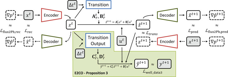
FIGURE 5. Training diagram for E2CO with flux and well data loss functions (proposition 3).

One of the main advantages of E2CO, when compared to propositions 1 and 2, is that here we do not rely on the state variables in the original space to predict well data. Instead of this, E2CO uses the state on the reduced space to create matrices ${\mathbf{C}}_r^t$ and ${\mathbf{D}}_r^t$ and uses a control system approach to estimate the output data. This resembles the case of system identification as in the control system community.

2.5 Training Versus Prediction

The diagrams presented in Figures 2–5 are used to train each proposed method’s networks. In these diagrams, the loss functions have an important role in the training procedure. They are defined to provide information about the system dynamics and honor the physics presented in the reservoir simulation process.

When the training procedure is finished, and the neural network parameters (weights, bias, and filters) are optimally found, it is time to use them to predict the system behavior. The prediction diagrams are significantly simpler than the training ones. The prediction diagram for propositions 1 and 2 is presented in Figure 6. In this figure, the time evolution happens in the latent space (z), potentially reducing the computational cost of the prediction step. However, to predict well data using propositions 1 and 2, it is necessary to have the state on the original space (x) at each desired time step to predict the well data at that time. That being said, one can note that it is necessary to pass ${\widehat{z}}^{t+1}$ through the decoder to calculate ${\widehat{x}}^{t+1}$ and further apply the Peaceman equation to calculate well data ${\widehat{y}}^{t+1}$ on each time step. The application of the decoder to predict the well data can lead to a computational cost increase.

FIGURE 6

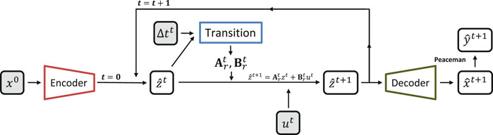
FIGURE 6. E2C prediction diagram (propositions 1 and 2).

For proposition 3, there is no need to decode the latent space since the well data is generated on that latent space using a specific network for this purpose (Transition Output). Figure 7 shows that both the state time evolution and the well data estimation happen in latent space. On proposition 3, the decoder’s use is limited to the cases where one would like to estimate the state on the original space (x).

FIGURE 7

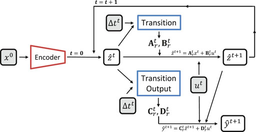
FIGURE 7. E2CO prediction diagram (proposition 3).

2.6 Neural Networks Structure

In the following sections, we describe the networks used in each part of the proposed models. The structure of the networks used here is very similar to the ones used in [2]. The three proposed ways of calculating well data use the same elements described in this section. Although the elements are the same, each proposed method’s parameters will differ due to the different model/network structure and different loss functions used in the training procedure.

2.6.1 Encoder

The encoder is built with a series of encoding blocks followed by residual convolutional blocks and a dense (fully connected layer), as depicted in Figure 8 (top).

FIGURE 8

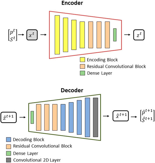
FIGURE 8. Encoder structure (top) and Decoder structure (bottom) (both adapted from [2]).

The main idea of the encoder structure is to transform the state variables on the original space x to the latent space z. The dimension of the latent space $l_z$ is smaller than the dimension of the original space $l_x$. To keep things in perspective the numerical model we will present next has $l_x=60\times 60\times 2=7200$ states and $l_z=50$.

Each encoding block comprises a convolutional 2D layer, followed by batch normalization and a ReLU (Rectified Linear Unit) activation function, as presented in Figure 9 (top). Although the structure of each encoding block is the same, the dimension of each block will change to be able to reduce the dimension of the encoder input. This dimension reduction is pictorially presented in Figure 8. The dimensions of each component used in this work will be presented later.

FIGURE 9

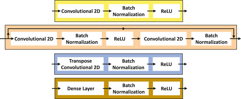
FIGURE 9. From top to bottom: Encoding block (top), Residual block, Decoding block, and Transformation block (bottom) (Adapted from [2]).

The residual convolutional blocks also have a convolutional 2D layer, followed by batch normalization and a ReLU, adding another convolutional 2D layer and batch normalization, as presented in Figure 9. It is possible to observe a link between the input and the output of the residual convolutional blocks. This is the characteristic of a residual block. It is built in this way mainly to avoid gradient vanishing during the training procedure.

2.6.2 Decoder

The decoder will work as an inverted encoder, where its main purpose is to transform the state variables in latent space z into the original space x. Its structure is composed of a dense (fully connected) layer, followed by three residual convolutional blocks, four decoding blocks, and a convolutional 2D layer, as presented in Figure 8 (bottom).

The residual convolutional block used in the decoder has the same structure as the used on the encoder. The decoding block (Figure 9) comprises a transpose convolutional 2D layer, batch normalization, and ReLU. In [2], the decoding block has a sequence of unpooling, padding, and convolution layers; here we replace this with a transpose convolutional layer.

2.6.3 Transition

The transition network is composed of two transformation blocks, followed by two dense layers directly connected to the output of the last transformation block. The output of these dense layers is reshaped to create the matrices ${\mathbf{A}}_r^t$ and ${\mathbf{B}}_r^t$. The transition network is presented in Figure 10 (left).

FIGURE 10

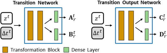
FIGURE 10. Transition network (left) (Adapted from [2]) and Transition Output network (right).

Although the authors in [2] used three transformation blocks, we will use two as proposed on one example from the original E2C model [1]. The transformation block (Figure 9 (bottom)) is composed of a dense layer with batch normalization followed by a ReLU activation layer.

2.6.4 Transition Output

The transition output network (Figure 10 (right)), used on our proposition 3, has a very similar structure compared with the transition network. The dimension of the dense layer in the transformation blocks will differ between these two networks. This will be detailed in the following section. Still, it is intuitive to think that the transition output network may require layers with smaller dimensions than the transition network. The transition network output is the matrices ${\mathbf{A}}_r^t$ and ${\mathbf{B}}_r^t$, which have sizes defined by the system input/state. On the other hand, the sizes of ${\mathbf{C}}_r^t$ and ${\mathbf{D}}_r^t$ depend on the dimensions of system input/output, which usually has lower dimensions when compared to the input/state.

2.7 Neural Networks Implementation

We implemented all the methods proposed here using Python 3.7.4 [26] and the framework TensorFlow 2.3.1 [27] with Keras API [28]. The dimensions of layers, number and size of filters, and output size of each block on the encoder and decoder used are presented in Tables 1 and 2.

TABLE 1

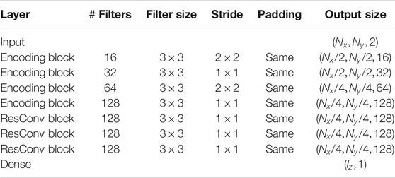
TABLE 1. Encoder architecture.

TABLE 2

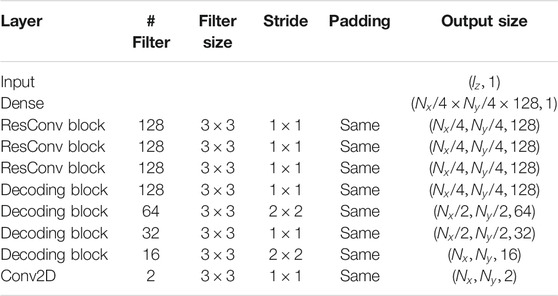
TABLE 2. Decoder architecture.

The transformation block has dimension of $n_{\text{Trans}}=200$ for the transition network, and the last dense layers before the matrices calculations have dimensions of $l_z^2$ for $A_r^t$ and $l_z\left(n_i+n_p\right)$ for $B_r^t$, where $n_i$ and $n_p$ are, respectively, the number of injector and producer wells. The output of these dense layers is then reshaped to match each matrix dimension. For the transition output network we are using $n_{\text{Trans}\_\text{WD}}=20$ for the transformation block dimension, and the last dense layers have dimensions of $l_z\left(n_i+2n_p\right)$ for $C_r^t$ and $\left(n_i+n_p\right)\left(n_i+2n_p\right)$ for $D_r^t$.

We used the Adam optimization algorithm with a learning rate of $1\times {10}^{-4}$ during the training procedure with a batch size of 4. The sample is randomly selected to compose the training batch. We run the training procedure for 100 epochs.

We initially trained our models on CPUs. However, we change to GPUs since the speed up is expressive. We provide in Table 3 a non-rigorous estimation of the training time, where it is possible to see the differences between training on CPU and GPU. More details on the GPUs NVIDIA Tesla used can be found on www.hprc.tamu.edu.

TABLE 3

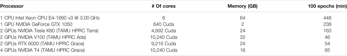
TABLE 3. Proposition 3 training time comparison for different hardware (CPUs and GPUs).

2.7.1 Non-determinism

During the initial implementation of the methods proposed here, we noticed that if we repeat the same training procedure twice in the same machine with the same input and parameters, we will end up with different networks, and this will lead to different predictions and different error estimations. Although this can be understood as a native characteristic of the neural network training procedure, this can increase the complexity of comparing different methods since each method’s results can change based on an uncontrollable variable.

Some of the non-determinism sources are layers weight initialization, kernel weights initialization, and the order of models to be part of the training batch. When training on GPU, some other sources can happen when using convolutional, pooling, and upsampling layers. All these sources are discussed in [29], which provides a solution for most of these sources of non-determinism. Here we used this method provided, and we can reproduce the training results for the same input and parameters.

2.7.2 Normalization

We used normalization to treat our input data from the state and the well data and also during the loss functions calculations. For each quantity, normalization parameters (min and max) are defined and used on this quantity over the training and prediction procedures. The normalization used here is:

${\mathcal{Q}}_{\text{NORM}}=\frac{\mathcal{Q}-{\mathcal{Q}}_{\text{min}}}{{\mathcal{Q}}_{\text{max}}-{\mathcal{Q}}_{\text{min}}},(29)$

where $\mathcal{Q}$ is the quantity to be normalized.

The minimum and maximum values for each quantity were selected from the input state (quantities: pressures and saturations), from the well data (quantities: well bottom hole pressure, the oil flow rate, and the water flow rate), and from the well controls (quantities: the water injection rate and well bottom hole pressure).

We also normalized values for the loss functions calculation. When applying Eqs 18 and 16, we use normalized values of state pressures and saturations. The same is valid for Eq. 24 where we used normalized values for well bottom hole pressure, the oil rate, and the water rate.

Here, we introduce the use of a normalized flux loss function. We first calculate the minimum and maximum flux from the input state and use them to normalize the flux loss function. This is valid for the single-phase loss function (Eqs. 21 and 22) and the two-phase (Eqs. 26 and 27), where we calculate maximum and minimum values for oil and water flux. By doing this, we expect not to need to use weight terms on these loss functions, like the ones used in [2]. This can potentially reduce the number of hyperparameters to be chosen on the training procedures.

3 Data Generation and Assessment

In this section, the simulation model used to generate state and well data is described, followed by the details on the training and validation data sets’ generation. We then show how we evaluate each trained model’s quality using the validation set by calculating the relative error.

3.1 Numerical Simulation

We utilized a commercial numerical reservoir simulator (IMEX from [30]) to generate the data employed on the training and validation steps of our propositions. However, any commercial off-the-shelf reservoir simulator can be used to train our model. A Cartesian grid with $60\times 60\times 1$ gridblocks and an oil–water fluid model were used. A fixed permeability field was generated and is presented in Figure 11 (left). The relative permeability curves used in the simulation model are shown in Figure 11 (right).

FIGURE 11

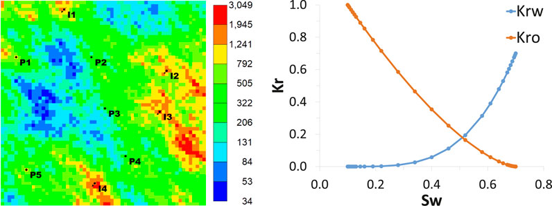
FIGURE 11. Permeability map (mD) (left) and Relative permeability curves (right).

The model has five producers and four injector wells. The producer wells are controlled by bottom hole pressure (BHP), and the injectors are controlled by the water injection rate. This model runs through 2,000 days, changing controls every 100 days. Some properties used in the simulation model are presented in Table 4.

TABLE 4

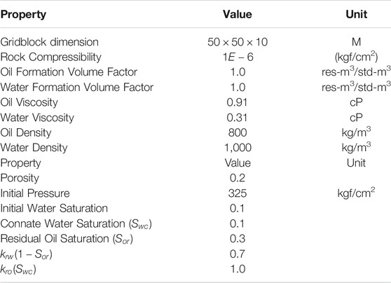
TABLE 4. Reservoir simulation model properties.

3.2 Data Sets

The objective of constructing a fast proxy model is to eventually connect it to control optimization frameworks whereby multiple calls of the surrogate model are used to determine a control set that optimizes an objective function (e.g., Net Present Value and sweep efficiency). In this case, we expect that our proxy might have the competence to predict well data under different sets of controls, which is usually unknown before the optimization is complete. To mimic the behavior of a varying input setting, we will use 300 simulations to train the proposed models, and each simulation will run through 20 time periods.

For the producers, the bottom-hole pressure was sampled over a uniform distribution $\mathcal{U}\left(\mathrm{260,275}\right)$ kgf/cm². To avoid having the same volume of water injected in all control sets, we used a different approach to create the injectors controls. For each control set i, we sampled a base injection rate $q_{inj\_base,i}\sim \mathcal{U}\left(\mathrm{300,950}\right)$ m³/day, and for each time period t, we sampled a perturbation $q_{inj\_pert,i,t}\sim \mathcal{U}\left(-\mathrm{80,90}\right)$ m³/day. The injection flow rate is then calculated as $q_{inj}\left(i,t\right)=q_{inj\_base,i}+q_{inj\_pert,i}^t$.

In Figure 12 we present an example of the injectors controls where readers can confirm the injection rate variability. The variability in the producer’s controls can be observed in Figure 13.

FIGURE 12

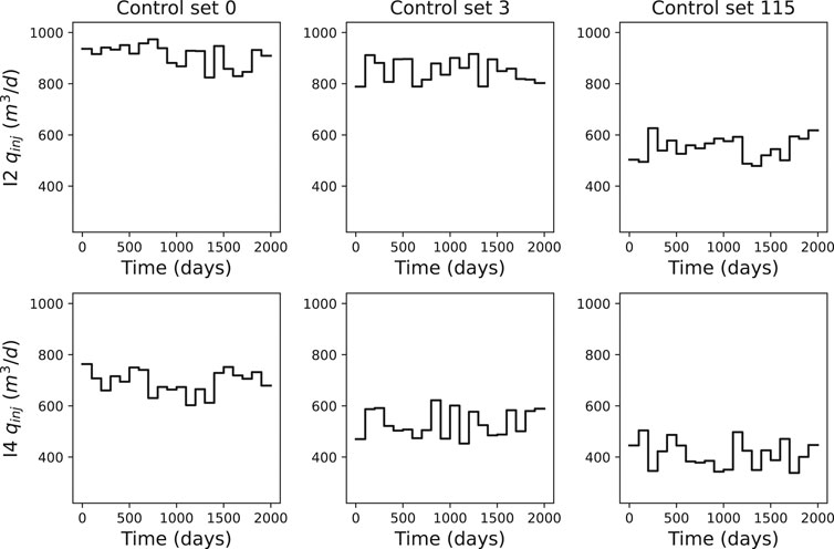
FIGURE 12. Injection water flowrate controls examples for wells I2 (first row) and I4 (second row) where each column represents a control set.

FIGURE 13

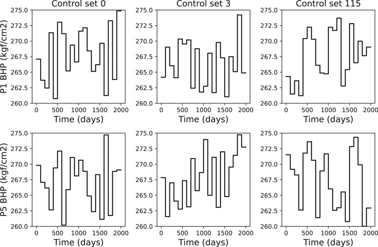
FIGURE 13. Producers BHP controls examples for wells P1 (first row) and P5 (second row) where each column represents a control set.

Using each one of the 300 control sets generated, we run the reservoir simulator and store the state (pressure and water saturation) at each one of the 20 time periods. The training set will be composed by 6,000 samples, each one containing:

• $x^t\to$ state on timestep t

• $x^{t+1}\to$ state on timestep $t+1$

• $u^t\to$ controls on timestep t

• $\text{Δ}{t}^t\to$ duration of timestep t

• $y^{t+1}\to$ well data on timestep $t+1$

In the case presented here, $t=\mathrm{0,1},\dots ,19$, where $t=0$ represents the initial state that also needs to be stored as the first snapshot of the state ($x^0$). The validation set contains 100 control sets that will create 2,000 samples. The validation set generation follows a similar approach but with a different random number generator seed. This is to enforce that training and validation are performed using different control inputs.

3.3 Model Evaluation

Each proposition (propositions 1 to 3, as constructed before) was trained as described in Section 2.7 using the training data set. We then used the models (networks) trained for each proposition on the prediction architecture, as shown in Figures 6, 7, and evaluated each model’s quality on the validation set. We also used this validation set to choose the better hyperparameters for each model. This is a tedious but necessary step in looking for a low prediction error model.

3.3.1 Error Definition

In this section, we present the definitions of relative error used to evaluate our model’s accuracy. Most of these definitions are similar to the ones defined in [2]. For a single producer wells (p), the relative error in the water and oil rates is defined as $e_w^p$ and $e_o^p$ that in a general way can be written as:

$e_j^p=\frac{{\displaystyle {\int }_0^T\left|{\widehat{q}}^{j,p}\left(t\right)-q_{\text{HFS}}^{j,p}\left(t\right)\right|dt}}{{\displaystyle {\int }_0^T\left|q_{\text{HFS}}^{j,p}\left(t\right)\right|dt}}.$

The error for all producer wells can be defined as:

$E_o=\frac{1}{n_p}\stackrel{n_p}{{\displaystyle \sum }_{p=1}}{e}_o^p,(30)$

$E_w=\frac{1}{n_p}\stackrel{n_p}{{\displaystyle \sum }_{p=1}}{e}_w^p,(31)$

where $j=o,w$ stands for the oil and water phases, respectively, and HFS stands for high-fidelity solution (numerical reservoir simulation run). The upper hat ($\widehat{\mathrm{ }}$) stands for estimated and is related to the output of the 3 propositions on how to estimate well data.

A similar equation can be built for the bottom hole pressure of an injector well (i), as given below:

$e_{\text{BHP}}^i=\frac{{\displaystyle {\int }_0^T\left|{\widehat{p}}^i\left(t\right)-p_{\text{HFS}}^i\left(t\right)\right|dt}}{{\displaystyle {\int }_0^T\left|p_{\text{HFS}}^i\left(t\right)\right|dt}}.$

The error for all injector wells can be calculated as:

$E_{\text{BHP}}=\frac{1}{n_i}{\displaystyle \sum }_{i=1}^{n_i}{e}_{\text{BHP}}^i,(32)$

where $n_i$ is the number of injector wells. We defined a relative error for the cumulative flowrates as:

$e_{\text{cum},j}^p=\frac{\left|{\widehat{Q}}^{j,p}-Q_{\text{HFS}}^{j,p}\right|}{\left|Q_{\text{HFS}}^{j,p}\right|},$

where $j=o,w$ and Q is the cumulative rate, and for all the producer we define:

$E_{\text{cum},j}=\frac{1}{n_p}\stackrel{n_p}{{\displaystyle \sum }_{p=1}}{e}_{\text{cum},j}^p(33)$

We also define a relative error in terms of the primary variables (pressures and water saturations) as:

$E_v=\frac{{\displaystyle {\sum }_{k=1}^{n_b}{\displaystyle {\int }_0^T\left|{\widehat{v}}^k\left(t\right)-v_{\text{HFS}}^k\left(t\right)\right|dt}}}{{\displaystyle {\sum }_{k=1}^{n_b}{\displaystyle {\int }_0^T\left|v_{\text{HFS}}^k\left(t\right)\right|dt}}},(34)$

where $v_k$ denotes the state variable at grid block k (pressure $p^k$ or water saturation $S^k$), and $n_b$ is the number of grid blocks in the numerical reservoir simulation grid.

3.3.2 Hyper-Parameters Tuning

The process of obtaining predictive neural networks with architecture like those used on the proposed methods is not straightforward. There are no mysteries in the training procedure itself. However, several hyper-parameters need to be selected before training, for example, the training batch size, number of epochs, and the learning rate. The choice of the best set of hyper-parameters is challenging, and the authors could not find a well-defined procedure on how to do it. To better choose the hyper-parameters, we have to proceed with full training and then using the validation data set, predict the outputs of this trained network to analyze the error of this choice. We should now repeat this process with another set of hyper-parameters to find the one that provides a smaller prediction error.

Looking for isolating each parameter’s influence, we run isolated tuning, where each tuning run will consist of trying some values of a hyper-parameter and fixing the others. For example, trying to find the best learning rate (for ADAM’s algorithm) we run the training and prediction for the values $1\times {10}^{-5}$, $1\times {10}^{-4}$, $1\times {10}^{-3}$, $1\times {10}^{-2}$, and $1\times {10}^{-1}$. The lowest error in estimating the well data was obtained with $1\times {10}^{-4}$. Now, this value will be fixed on the other tuning runs. We understand that this might not be the optimal approach. However, using a grid search-like method is not feasible since to span the hyper-parameters space would be high computationally costly.

Using a batch size of four is a significantly better choice than using 20 or 100. Larger batch sizes reduce the training process’s duration; however, it increases the prediction error in our case. The samples were shuffled to build the batch. This approach worked better than building the batch following the time sequence.

The number of epochs used on the training runs was not considered as a hyper-parameter. We run all our training processes for 100 epochs, saving the network at every 10 epochs. In some cases, we observed that the network that produces the lowest prediction well data error is not obtained after epoch 100, as we expected. This was observed during some hyper-parameters tuning runs. However, when the best hyper-parameter set was found on the specific tuning run, it was always on the last epoch. This might be interpreted as when we are far from the best hyper-parameter, the training procedure presents some instability. It is noteworthy that along the training process, the total loss function keeps decreasing at each epoch. However, the error we are analyzing here is the prediction error defined in a previous section, which is not directly related to the total loss function used on the training procedure.

We tried to find the dimension of the latent space $l_z$ that produces the lowest well data prediction error by changing $l_z=\mathrm{10,20,50}$, and 100, and the smallest error was obtained by using $l_z=50$. The dimension of the dense layer on the transformation blocks was changed between values $\mathrm{50,100,200}$, and 500, and the lowest error was found when the dimension was 200. For the E2CO, the dense layer’s dimension on the transformation blocks in the transition output network was varied between $\mathrm{10,20,100}$, and 200, and the best value was 20.

The most challenging tuning was on weights applied to the loss functions. Our training procedure relies on the combination of loss functions, and how these functions are optimally weighted to build the total loss function is not an easy task. Here was mentioned that we used normalization of inputs, outputs, and components of loss functions to avoid the need to tune the loss function weights. We initially tried to train our models with the loss functions not weighted to compose the total loss function, but after some tests, we realize that there was room for improvement in weighing them.

For proposition 1, we can define the total loss function as:

${\mathrm{ℒ}}_{\text{prop}1}={\mathrm{ℒ}}_{\text{rec}}+{\mathrm{ℒ}}_{\text{pred}}+{\mathrm{ℒ}}_{\text{trans}}+{\gamma }_{\text{flux}}{\mathrm{ℒ}}_{\text{flux}}+{\gamma }_{\text{p}\_\text{pres}}{\mathrm{ℒ}}_{\text{p}\_\text{pres}},(35)$

where ${\gamma }_{\text{flux}}$ is the weight applied to the flux loss function (Eq. 23) and ${\gamma }_{\text{p}\_\text{pres}}$, is the weight applied to the loss function of pressure in the producers well gridblocks. This resembles the way the authors in [2] defined the loss function. The values that produces a smaller prediction error are ${\gamma }_{\text{flux}}=5$ and ${\gamma }_{\text{p}\_\text{pres}}=0$. We tried several values for ${\gamma }_{\text{p}\_\text{pres}}$, but the best results where obtained with zero for this weight.

For proposition 2, we need to add the well data loss function (${\mathrm{ℒ}}_{\text{well}\_\text{data}2}$), so the total loss function will become:

${\mathrm{ℒ}}_{\text{prop}2}={\mathrm{ℒ}}_{\text{rec}}+{\mathrm{ℒ}}_{\text{pred}}+{\mathrm{ℒ}}_{\text{trans}}+{\gamma }_{\text{flux}2\text{Ph}}{\mathrm{ℒ}}_{\text{flux}2\text{Ph}}+{\gamma }_{\text{well}\_\text{data}2}{\mathrm{ℒ}}_{\text{well}\_\text{data}2},(36)$

where ${\gamma }_{\text{flux}2\text{Ph}}$ is the weight applied to the two phase flux loss function and ${\gamma }_{\text{well}\_\text{data}2}$ represents the weight applied to the well data loss function.

For the E2CO (proposition 3) we can define the total loss function as:

${\mathrm{ℒ}}_{\text{E}2\text{CO}}={\mathrm{ℒ}}_{\text{rec}}+{\mathrm{ℒ}}_{\text{pred}}+{\mathrm{ℒ}}_{\text{trans}}+{\gamma }_{\text{flux}}{\mathrm{ℒ}}_{\text{flux}}+{\gamma }_{\text{well}\_\text{data}3}{\mathrm{ℒ}}_{\text{well}\_\text{data}3}.(37)$

We tried variations of propositions 2 and 3 total loss functions using different flux loss functions: one-phase, two-phase, and no flux loss. We also tried to give more weight to the state variables (pressure and saturation) on the well grid blocks. This analysis was applied to the injectors and producers’ well gridblocks. We tested several combinations of different weights for a loss function that looks at the mismatch between the predicted and the true values of the wells gridblock state variables. These loss functions can be identified as ${\mathrm{ℒ}}_{\text{p}\_\text{pres}}$, ${\mathrm{ℒ}}_{\text{p}\_\text{sat}}$, ${\mathrm{ℒ}}_{\text{i}\_\text{pres}}$, and ${\mathrm{ℒ}}_{\text{i}\_\text{sat}}$, and there respective weights are ${\gamma }_{\text{p}\_\text{pres}}$, ${\gamma }_{\text{p}\_\text{sat}}$, ${\gamma }_{\text{i}\_\text{pres}}$, and ${\gamma }_{\text{i}\_\text{sat}}$. We expected that this would improve the model’s ability to predict well data, but this was not true for all cases.

For proposition 2, the best results were obtained using ${\gamma }_{\text{flux}2\text{Ph}}=1.0$, ${\gamma }_{\text{well}\_\text{data}2}=1.0$, and ${\gamma }_{\text{p}\_\text{pres}}={\gamma }_{\text{p}\_\text{sat}}={\gamma }_{\text{i}\_\text{pres}}={\gamma }_{\text{i}\_\text{sat}}=0$.

For E2CO (proposition 3), the best results were obtained using single phase loss function, ${\gamma }_{\text{flux}1\text{Ph}}=0.1$, ${\gamma }_{\text{well}\_\text{data}3}=1.0$, ${\gamma }_{\text{p}\_\text{pres}}=0.01$, and ${\gamma }_{\text{p}\_\text{sat}}={\gamma }_{\text{i}\_\text{pres}}={\gamma }_{\text{i}\_\text{sat}}=0$.

The choice of best hyperparameters set for each proposition was defined by analyzing the validation set’s total prediction error. We used the summation of the median of the errors defined by Eqs 30–34, here defined as total prediction error, to choose the best hyperparameters set.

3.3.3 Training Size Sensibility

We are interested in understanding the performance of the two proposed methods when less data is available for training or the resources available for the training are limited. Using the best set of hyperparameters described in the previous session, 3 training procedures were conducted varying the training set size for each model. The original training set size was 6,000 samples, and we also trained with 4,000 samples and 2,000 samples (each one corresponding to 300, 200, and 100 controls sets). Figure 14 shows the relative error median over the validation set for the oil rate, the water rate, and BHP for each proposed method. A similar trend for all the curves can be observed, and as expected, when the number of training samples is reduced, the estimation error on the validation set increases. Important to note that for the oil rate and BHP, the E2CO method presents lower values for relative error when reducing the training set size. Proposition 1 provides slightly better results only for the water rate with the lowest numbers of training samples.

FIGURE 14

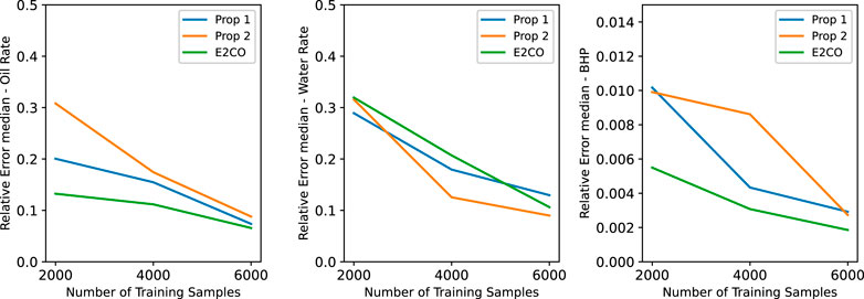
FIGURE 14. Validation set error for different training set sizes.

4 Results

This section will present a validation set error comparison between the best hyperparameters set for each of the propositions. We finish this section by comparing the methods by showing well data and states outputs of a specific control combination from the validation set.

We defined the best hyperparameters set based on the total error median over the validation set for all the three proposed models on the hyperparameters tuning procedure. We can now analyze the performance of these three models by comparing the error for each item analyzed. In Figure 15 we present the error for well data, where this box plot represents the distribution of the relative error on the validation set. The bottom and top limits of each box represent 25th, and 75th percentile errors, the orange line inside the box is the median of the distribution.

FIGURE 15

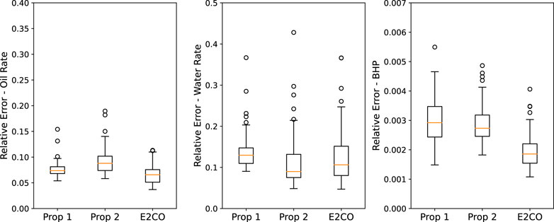
FIGURE 15. Validation set error on the 3 propositions for oil rate (left plot), water rate (middle plot) and BHP (right plot).

Analyzing oil rate relative error in Figure 15, it is possible to conclude that E2CO overcome propositions 1 and 2. For the water rate and bottom hole pressure, we obtained a smaller error for both E2CO and proposition 2 than proposition 1. However, the E2CO estimation errors for the water rate are higher than proposition 2. We impute this pour performance to failure on estimating water rate before water breakthrough. We present and discuss this problem better in Figure 16.

FIGURE 16

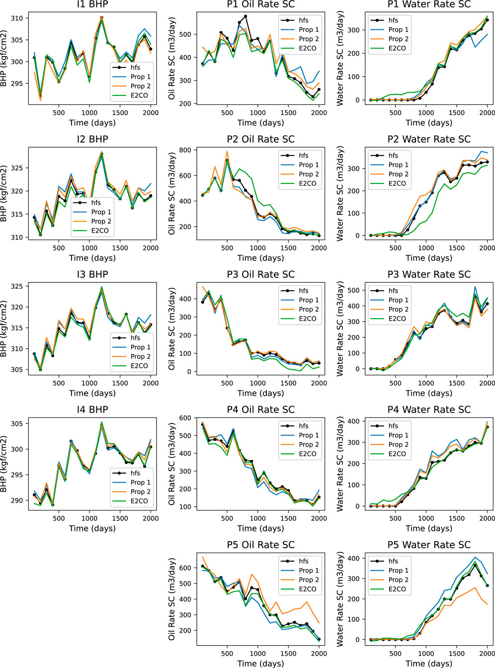
FIGURE 16. Well data prediction for validation sample 6.

A similar analysis can be built for cumulative flow rates, as in Figure 17. It is possible to observe that proposition 2 and E2CO overcome the cumulative water flow rates prediction ability of proposition 1. The same figure shows that the cumulative oil rate is better predicted by proposition 1. We can also visualize the cumulative errors in a scatter plot of cumulative flow rate plots (Figure 18), where it is possible to confirm the previous figure’s analysis.

FIGURE 17

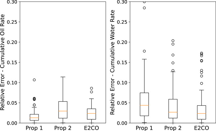
FIGURE 17. Validation set error for cumulative oil (left plot) and cumulative water (right plot) production.

FIGURE 18

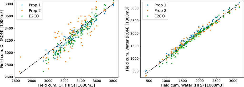
FIGURE 18. Cumulative oil (left plot) and water (right plot) production.

The error on the state variables is presented in Figure 19. We can observe that both E2CO and proposition 2 overcome the state estimation ability of proposition 1. During the development of both E2CO and proposition 2, we aimed on getting accurate well data estimation; however, these results show that we are also able to predict states. Proposition 2 has a lower estimation error, which can be assigned as a benefit of using the 2 phase flux loss function proposed in this research.

FIGURE 19

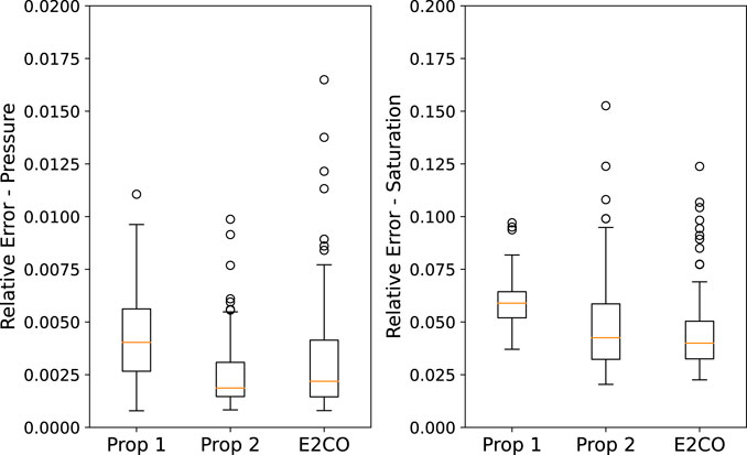
FIGURE 19. Validation set error on the 3 propositions for pressure (left plot) and saturation (right plot).

We now present in Figure 16 the predicted well data of one validation sample for all the three models. It is noteworthy that E2CO has some problems with water flowrate estimation, mainly before the water breakthrough. This could be addressed by narrowing its values to only positive values, which is an easy procedure. One can check the saturation on the well gridblock, and if saturation is not higher than the connate water saturation, set its value to zero. This will compel the need to rebuild the full state. Here, we did not implement any of these procedures, and the results presented are exactly the ones generated by the E2CO method.

The pressure and water saturation maps for the last predicted time step using one validation sample in Figures 20, 21. The maps did not show significant differences; however, the error map for pressure shows lower values for proposition 2 and E2CO. For saturation error map, proposition 2 shows higher errors in a southern area.

FIGURE 20

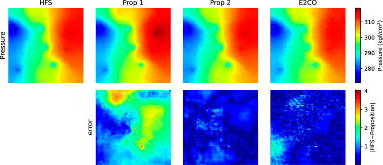
FIGURE 20. Pressure map for the last predicted time step of validation sample 3.

FIGURE 21

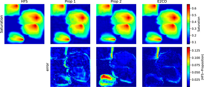
FIGURE 21. Water saturation map for the last predicted time step of validation sample 3.

5 Conclusion

This work presents a new framework to develop proxy models for reservoir simulation. Our method is based on a deep convolutional autoencoder and control system approach. Our development was inspired by the E2C-ROM method (named proposition 1) proposed by [2]. In this study, we leverage its capability of state reconstruction by adding to it a well data (output) loss function on the training procedure (proposition 2). Additionally, we introduce E2CO—Embed to Control and Observe (proposition 3)—as an alternative approach to calculate the model output by having a specific neural network to capture the relation between reduced state, controls, and outputs. The methods developed here can be related to the reduced-order modeling technique POD-TPWL.

We applied our proposed new architecture on a two-phase 2D synthetic reservoir simulation model running on a commercial reservoir simulation. The results of proposition 2 and E2CO applications in our synthetic case presented improvements when compared with E2C-ROM. The well data estimation errors on the validation set are generally more accurate and present less variability using the two proposed methods, especially the estimations of oil rate and cumulative oil and water production. Proposition 2 has also shown slightly better results, but its limitations are the same as the E2C-ROM: the need to reconstruct the full state to estimate the well data. On the other hand, our new E2CO methodology can predict well data using the reduced state directly without being estimated by the Peacemen formula.

Although we have shown the advantages and limitations of our proposed methods using a 2D reservoir, their performance and generalizations need to be tested on more realistic scenarios with larger and more complex models (black-oil or compositional). The explosion on the number of state variables’ and, thus, the model dimension may lead to more challenging well data estimation. It may be necessary to increase the dimension of the reduced space $l_z$, and the neural network dimension responsible for generating the linearized system matrix.

Data Availability Statement

The raw data supporting the conclusions of this article will be made available by the authors, without undue reservation.

Author Contributions

All authors listed have made a substantial, direct, and intellectual contribution to the work and approved it for publication.

Conflict of Interest

Author EC is employed by the company Petrobras.

The remaining authors declare that the research was conducted in the absence of any commercial or financial relationships that could be construed as a potential conflict of interest.

Publisher’s Note

All claims expressed in this article are solely those of the authors and do not necessarily represent those of their affiliated organizations, or those of the publisher, the editors and the reviewers. Any product that may be evaluated in this article, or claim that may be made by its manufacturer, is not guaranteed or endorsed by the publisher.

Acknowledgments

Portions of this research were conducted using the advanced computing resources provided by Texas A&M High-Performance Research Computing. The first author also acknowledges all the support provided by Petroleo Brasileiro S.A. The funder Petroleo Brasileiro S.A was not involved in the study design, collection, analysis, interpretation of data, the writing of this article or the decision to submit it for publication. The authors thank Zhaoyang Larry Jin and Louis J. Durlofsky for helpful discussions regarding their E2C implementation and for providing codes associated with their published study.

References

1. Watter, M, Springenberg, JT, Boedecker, J, and Riedmiller, M. Embed to Control: A Locally Linear Latent Dynamics Model for Control from Raw Images. arXiv:1506.07365 (2015).

2. Jin, ZL, Liu, Y, and Durlofsky, LJ. Deep-learning-based Surrogate Model for Reservoir Simulation with Time-Varying Well Controls. J Pet Sci Eng (2020) 192:107273. doi:10.1016/j.petrol.2020.107273

CrossRef Full Text | Google Scholar

3. Jansen, JD. A Systems Description of Flow through Porous Media. In: SpringerBriefs in Earth Sciences. Heidelberg: Springer International Publishing (2013). doi:10.1007/978-3-319-00260-6

CrossRef Full Text | Google Scholar

4. Antoulas, AC. Approximation of Large-Scale Dynamical Systems. In: Advances in Design and Control. Philadelphia: Society for Industrial and Applied Mathematics (2005). doi:10.1137/1.9780898718713

CrossRef Full Text | Google Scholar

5. Gildin, E, Klie, H, Rodriguez, A, Wheeler, MF, and Bishop, RH. Projection-Based Approximation Methods for the Optimal Control of Smart Oil Fields. In: ECMOR X - 10th European Conference on the Mathematics of Oil Recovery. Houten: European Association of Geoscientists & Engineers (2006). p. 00032. ISSN: 2214-4609. doi:10.3997/2214-4609.201402503

CrossRef Full Text | Google Scholar

6. Cardoso, MA, and Durlofsky, LJ. Linearized Reduced-Order Models for Subsurface Flow Simulation. J Comput Phys (2010) 229:681–700. doi:10.1016/j.jcp.2009.10.004

CrossRef Full Text | Google Scholar

7. Jin, ZL, and Durlofsky, LJ. Reduced-order Modeling of CO2 Storage Operations. Int J Greenhouse Gas Control (2018) 68:49–67. doi:10.1016/j.ijggc.2017.08.017

CrossRef Full Text | Google Scholar

8. Chaturantabut, S, and Sorensen, DC. Application of POD and DEIM on Dimension Reduction of Non-linear Miscible Viscous Fingering in Porous media. Math Comp Model Dynamical Syst (2011) 17:337–53. doi:10.1080/13873954.2011.547660

CrossRef Full Text | Google Scholar

9. Tan, X, Gildin, E, Florez, H, Trehan, S, Yang, Y, and Hoda, N. Trajectory-based DEIM (TDEIM) Model Reduction Applied to Reservoir Simulation. Comput Geosci (2019) 23:35–53. doi:10.1007/s10596-018-9782-0

CrossRef Full Text | Google Scholar

10. Lee, JW, and Gildin, E. A New Framework for Compositional Simulation Using Reduced Order Modeling Based on POD-DEIM. In: SPE Latin American and Caribbean Petroleum Engineering Conference. Richardson: Society of Petroleum Engineers (2020). doi:10.2118/198946-MS

CrossRef Full Text | Google Scholar

11. Jiang, R, and Durlofsky, LJ. Implementation and Detailed Assessment of a GNAT Reduced-Order Model for Subsurface Flow Simulation. J Comput Phys (2019) 379:192–213. doi:10.1016/j.jcp.2018.11.038

CrossRef Full Text | Google Scholar

12. Zubarev, DI. Pros and Cons of Applying Proxy-Models as a Substitute for Full Reservoir Simulations. In: SPE Annual Technical Conference and Exhibition. New Orleans: Louisiana: Society of Petroleum Engineers (2009). doi:10.2118/124815-MS

CrossRef Full Text | Google Scholar

13. Plaksina, T. Modern Data Analytics: Applied AI and Machine Learning for Oil and Gas Industry. UQcuzAEACAAJ: Google-Books-ID (2019).

14. Mishra, S, and Datta-Gupta, A. Applied Statistical Modelling and Data Analytics. Elsevier (2018). doi:10.1016/C2014-0-03954-8

CrossRef Full Text

15. Mohaghegh, SD. Shale Analytics: Data-Driven Analytics in Unconventional Resources. Springer International Publishing (2017). doi:10.1007/978-3-319-48753-3

CrossRef Full Text

16. Misra, S, Li, H, and He, J. Machine Learning for Subsurface Characterization. Elsevier (2020). doi:10.1016/C2018-0-01926-X

CrossRef Full Text

17. Sankaran, S, Matringe, S, Sidahmed, M, and Saputelli, L. Data Analytics in Reservoir Engineering. Richardson: Society of Petroleum Engineers (2020).

18. Chiuso, A, and Pillonetto, G. System Identification: A Machine Learning Perspective. Annu Rev Control Robot Auton Syst (2019) 2:281–304. doi:10.1146/annurev-control-053018-023744

CrossRef Full Text | Google Scholar

19. Ljung, L, Hjalmarsson, H, and Ohlsson, H. Four Encounters with System Identification. Eur J Control (2011) 17:449–71. doi:10.3166/ejc.17.449-471

CrossRef Full Text | Google Scholar

20. Aziz, K, and Settari, A. Petroleum Reservoir Simulation. London: Applied Science Publishers Ltd (1979).

21. Ertekin, T, Abou-Kassem, J, and King, G. Basic Applied Reservoir Simulation. Richardson: Society of Petroleum Engineering (2001).

22. Peaceman, DW. Interpretation of Well-Block Pressures in Numerical Reservoir Simulation(includes Associated Paper 6988). Soc Pet Eng J (1978) 18:183–94. doi:10.2118/6893-pa

CrossRef Full Text | Google Scholar

23. Zandvliet, MJ, Van Doren, JFM, Bosgra, OH, Jansen, JD, and Van den Hof, PMJ. Controllability, Observability and Identifiability in Single-phase Porous media Flow. Comput Geosci (2008) 12:605–22. doi:10.1007/s10596-008-9100-3

CrossRef Full Text | Google Scholar

24. Van Doren, JFM, Van den Hof, PMJ, Bosgra, OH, and Jansen, JD. Controllability and Observability in Two-phase Porous media Flow. Comput Geosci (2013) 17:773–88. doi:10.1007/s10596-013-9355-1

CrossRef Full Text | Google Scholar

25. Heijn, T, Markovinovic, R, and Jansen, J-D. Generation of Low-Order Reservoir Models Using System-Theoretical Concepts. SPE J (2004) 9:202–18. doi:10.2118/88361-PA

CrossRef Full Text | Google Scholar

26. Van Rossum, G, and Drake, FL. Python 3 Reference Manual. Scotts Valley, CA: CreateSpace (2009).

27. Abadi, M, Agarwal, A, Paul, B, Brevdo, E, Chen, Z, Craig, C, et al. Tensor Flow: Large-Scale Machine Learning on Heterogeneous Systems. TensorFlow (2015).

28. Chollet, F. Keras. TensorFlow (2015).

29. Riach, D. GitHub - NVIDIA/framework-determinism: Providing Determinism in Deep Learning Frameworks (2020).

30.CMG. IMEX, Black Oil & Unconventional Reservoir Simulator (2019).

Glossary

$\mathbf{A}$ Discretized state matrix

${\mathbf{A}}_c$ Continuous state matrix

${\mathbf{A}}_r$ Discretized reduced state matrix

$\mathbf{B}$ Discretized input matrix Formation volume factor

${\mathbf{B}}_c$ Continuous input matrix

${\mathbf{B}}_r$ Discretized reduced input matrix

BHP Bottom Hole Pressure

B Discretized input matrix Formation volume factor

$\mathbf{C}$ Discretized output matrix

${\mathbf{C}}_c$ Continuous output matrix

${\mathbf{C}}_r$ Discretized reduced output matrix

$\mathbf{D}$ Discretized feed-through matrix

${\mathbf{D}}_c$ Continuous feed-through matrix

${\mathbf{D}}_r$ Discretized reduced feed-through matrix

E2C Embed to Control

E2CO Embed to Control and Observe

$e_j^p$ Producer well p relative error of phase j flowrate

$E_o$ Relative oil flow rate error for all producers

$E_v$ Relative error for state variable v

$E_w$ Relative water flow rate error for all producers

$E_{\text{BHP}}$ Relative bottom hole pressure error for all injectors

$e_{\text{BHP}}^i$ Injector well i relative error of bottom hole pressure

$E_{\text{cum},j}$ Relative cumulative phase j flow rate error for all producers

$e_{\text{cum},j}^p$ Producer well p relative error for the phase j cumulative flow rate

h Height of the well grid block

HFS High Fidelity Simulation (Numerical Simulation)

k Permeability

$k_{r,j}$ Relative permeability to the phase j

$l_x$ Dimension of the state on the original space

$l_z$ Dimension of the state on the reduced space

${\mathrm{ℒ}}_{\text{flux},\text{pred}}$ Prediction Flux Loss Function

${\mathrm{ℒ}}_{\text{flux},\text{rec}}$ Reconstruction Flux Loss Function

${\mathrm{ℒ}}_{\text{flux}2\text{Ph},\text{pred}}$ Prediction Two phase Flux Loss Function

${\mathrm{ℒ}}_{\text{flux}2\text{Ph},\text{rec}}$ Reconstruction Two phase Flux Loss Function

${\mathrm{ℒ}}_{\text{flux}2\text{Ph}}$ Two phase Flux Loss Function

${\mathrm{ℒ}}_{\text{flux}}$ Flux Loss Function

${\mathrm{ℒ}}_{\text{pred}}$ Prediction Loss Function

${\mathrm{ℒ}}_{\text{rec}}$ Reconstruction Loss Function

${\mathrm{ℒ}}_{\text{i}\_\text{pres}}$ Loss function of the injectors gridblock pressure

${\mathrm{ℒ}}_{\text{i}\_\text{sat}}$ Loss function of the injectors gridblock saturation

${\mathrm{ℒ}}_{\text{p}\_\text{pres}}$ Loss function of the producers gridblock pressure

${\mathrm{ℒ}}_{\text{p}\_\text{sat}}$ Loss function of the producers gridblock saturation

${\mathrm{ℒ}}_{\text{trans}}$ Transition Loss Function

${\mathrm{ℒ}}_{\text{well}\_\text{data}2}$ Well data loss function for proposition 2

${\mathrm{ℒ}}_{\text{well}\_\text{data}3}$ Well data loss function for proposition 3

μ Viscosity

MOR Model Order Reduction

$n_i$ Number of injector wells

$n_p$ Number of producer wells

P Pressure

$\nabla p$ Pressure gradient of adjacent grid blocks

POD Proper Orthogonal Decomposition

ϕ Porosity

ρ Density

$q_{\text{inj}}$ Injection Water Rate

$q_o$ Oil Rate

$q_w$ Produced Water Rate

$r_o$ Well gridblock equivalent radius

$r_w$ Well bore radius

S Saturation

$S_w$ Water Saturation

SKIN Skin Factor

TPWL Trajectory Piecewise Linearization

u System input or control

WI Well index

x State on original space

$\dot{x}$ State time derivative

$\widehat{x}$ Estimated state on original space

y System output

$\widehat{y}$ Estimated observed data

${\gamma }_{\text{flux}}$ Weight applied to ${\mathrm{ℒ}}_{\text{flux}}$

${\gamma }_{\text{flux}2\text{Ph}}$ Weight applied to ${\mathrm{ℒ}}_{\text{flux}2\text{Ph}}$

${\gamma }_{\text{i}\_\text{pres}}$ Weight applied to ${\mathrm{ℒ}}_{\text{i}\_\text{pres}}$

${\gamma }_{\text{i}\_\text{sat}}$ Weight applied to ${\mathrm{ℒ}}_{\text{i}\_\text{sat}}$

${\gamma }_{\text{p}\_\text{pres}}$ Weight applied to ${\mathrm{ℒ}}_{\text{p}\_\text{pres}}$

${\gamma }_{\text{p}\_\text{sat}}$ Weight applied to ${\mathrm{ℒ}}_{\text{p}\_\text{sat}}$

${\gamma }_{\text{well}\_\text{data}2}$ Weight applied to ${\mathrm{ℒ}}_{\text{well}\_\text{data}2}$

${\gamma }_{\text{well}\_\text{data}3}$ Weight applied to ${\mathrm{ℒ}}_{\text{well}\_\text{data}3}$

z State on latent space

$\widehat{z}$ Estimated state on latent space