Supervised Learning Using Homology Stable Rank Kernels

1 Introduction

Topological data analysis (TDA) is a framework for analyzing data which is mathematically well-founded and with roots in algebraic topology. Through the use of persistent homology, TDA proposes to analyze datasets, often being high-dimensional and unstructured, where each observation is an object encoding some notion of a distance. An example of such an object is a point cloud with Euclidean distance. A convenient way of encoding distance objects is via Vietoris-Rips complexes [1]. Persistent homology transforms these complexes into so-called persistence modules and diagrams [2, 3]. These modules and diagrams encode geometrical aspects of the distance objects captured by homology. We thus regard the obtained persistence diagrams as summaries encoding geometrical features of the considered distance objects. In recent applications, and in such varied fields as bioinformatics [4] and finance [5], it has been shown that these summaries encode valuable information which is often complementary to that derived from non-topological methods.

The discriminative information contained in the persistent homology summaries makes them interesting in the context of machine learning, for instance to serve as inputs in supervised learning problems. The space of persistence diagrams lacks however the structure of a Euclidean, or more generally Hilbert space, often required for the development of machine learning (ML) methods. Furthermore, for inference purposes we also need to be able to consider probability distributions over topological summaries. Since for persistence diagrams we only have Fréchet means at our disposal [6, 7] inference is difficult.

Our aim in this article is to present how persistent homology can be combined with machine learning algorithms within a framework called hierarchical stabilization [8–10]. We will use hierarchical stabilization to define new persistence-based kernels and illustrate them on artificial and real-world datasets. This article is based in part on some of the results described in Jens Agerberg’s thesis [11].

Comparing and interpreting summaries produced by persistent homology should not just depend on their values but crucially also on the phenomena and the experiments that the considered datasets describe. Different phenomena might require different comparison criteria. It may not be optimal to consider only Bottleneck or Wasserstein distances to compare outcomes of persistent homology of diverse datasets obtained from a variety of different experiments. The ability to choose distances that fit particular experiments is required. We do not, however, plan to use these distances to compare persistence modules directly. Instead, quite essentially we use a chosen distance to transform, via the hierarchical stabilization process, the space of persistence modules into the space $\mathrm{ℳ}$ of (Lebesgue) measurable functions $\left[0,\mathrm{\infty }\right)\to (-\mathrm{\infty },\mathrm{\infty })$ with the $L_2$ distance. Thus each distance d on persistence modules leads to a function denoted by the symbol ${\widehat{\text{rank}}}_d:\text{Persistence modules}\to \mathrm{ℳ}$ called the stable rank. With the $L_2$ distance, $\mathrm{ℳ}$ is a Hilbert space and its scalar product provides an effective tool to study geometrical aspects of the image of ${\widehat{\text{rank}}}_d$, particularly those captured by measuring length, angles, and exploring orthogonality. Thus kernel machine learning methods, which are based on scalar products, are effective tools in exploring such geometrical features. Illustrating the effectiveness of this strategy for modeling with stable ranks is the aim of this paper.

Since the stable rank is stable with respect to d, the kernel formed can be seen as a similarity measure associated to d, of practical importance in several machine learning methods. In this framework, supervised learning consists of identifying these distances d for which structural properties of the training data are reflected by the geometry of its image in $\mathrm{ℳ}$ through the function ${\widehat{\text{rank}}}_d$. The strategy of looking for appropriate distances can only work if we are able to parametrize explicitly a rich subspace of distances on persistence modules. The hierarchical stabilization process builds on the discovery that such parametrization is possible using positive (Lebesgue) measurable functions $\left[0,\infty \right)\to \left(0,\infty \right)$ called densities. An organized search in the space of densities is beyond the scope of this article. The intention of this paper is to illustrate that by changing the density, the kernels can improve the accuracy in a supervised learning task.

Our method fits within the family of persistence based kernels [12], some of which also have parameters which can be optimized to fit a particular learning task [13]. However, a characteristic of our stable rank kernel is that it is defined on persistence modules rather than on persistence diagrams. A bar decomposition of the persistence modules is therefore useful but not essential for the definition of our kernel, which is readily generalisable to multi-parameter persistence.

2 Materials and Methods

2.1 Homological Simplification: From Data to Persistence Modules

Recall that a distance on a set X is a function $d:X\times X\to \left[0,\infty \right)$ which is symmetric $d\left(x,y\right)=d\left(y,x\right)$ and reflexive $d\left(x,x\right)=0$. It is a pseudometric if in addition it satisfies the triangular inequality $d\left(x,y\right)+d\left(y,z\right)\ge d\left(x,z\right)$. For example, by restricting a distance on the plane to a point cloud we obtain a finite distance space.

In this article we focus on data whose points are represented by finite distance spaces. This type of data is often the result of performing multiple measurements for each individual, representing these measurements as vectors, choosing a distance between the vectors, and representing each individual by a distance space. Encoding data points in this way reflects properties of the performed measurements accurately. That is an advantage but also a disadvantage as a lot of the complexity of the experiment is retained including possible noise, measurement inaccuracies, effects of external factors that might be irrelevant for the experiment but influence the measurements, etc. Because of this overwhelming complexity, to extract relevant information we need to simplify. Data analysis is a balancing act between simplifying, which amounts to ignoring some or often most of the information available, and retaining what might be meaningful for the particular task. In this article we study various simplifications based on homology.

The first step in extracting homology is to convert distance information into spatial information. We do that using so-called Vietoris-Rips complexes [1]. By definition the Vietoris-Rips complex ${\text{VR}}_{\mathit{ϵ}}\left(X,d\right)$, at scale ϵ in $\left[0,\infty \right)$, is a simplicial complex whose simplices are given by the non-empty finite subsets $\sigma \subset X$ for which $d\left(x,y\right)\le \mathit{ϵ}$ for every x and y in σ. Vietoris-Rips complexes form an increasing filtration as ${\text{VR}}_{\mathit{ϵ}}\left(X,d\right)\subset {\text{VR}}_{\tau }\left(X,d\right)$ when $\mathit{ϵ}\le \tau$. In the case X is finite, there is a finite sequence of parameters $0\le a_0\le \cdots \le a_l$ such that ${\text{VR}}_{\mathit{ϵ}}\left(X,d\right)\subset {\text{VR}}_{\tau }\left(X,d\right)$ may fail to be the equality only if $\mathit{ϵ}<a_i\le \tau$ for some i, i.e., the jumps in the Vietoris-Rips filtration can occur only when passing through some $a_i$. Such filtrations are called tame [8, 10].

The Vietoris-Rips filtration does not lose or add information about the distance space. It retains all the complexity of d. Thus, the purpose of this step is not to simplify, but rather to allow for the extraction of homology (see for example [14]). In this article we only consider reduced homology. The first step in extracting homology is to choose a field; for example, ${\mathbb{F}}_2$ with two elements. Homology in a given degree n, with coefficients in a chosen field F, converts a simplicial complex X into an F vector space $H_n\left(X\right)$. Homology is a functor which means that it also converts maps of simplicial complexes $f:X\to Y$ into linear functions $H_n\left(f\right):H_n\left(X\right)\to H_n\left(Y\right)$ such that $H_n\left(\text{id}\right)=\text{id}$ and $H_n\left(gf\right)=H_n\left(g\right)H_n\left(f\right)$ for any composable maps f and g. Homology encodes certain geometric features of the simplicial complex, for example the dimension of $H_0\left(X\right)$ is one less than the number of connected components of X, as the considered homology is reduced.

By applying homology to Vietoris-Rips complexes, we obtain a vector space $H_n\left({\text{VR}}_{\mathit{ϵ}}\left(X,d\right)\right)$ for every ϵ in $\left[0,\infty \right)$. By applying homology to the inclusions ${\text{VR}}_{\mathit{ϵ}}\left(X,d\right)\subset {\text{VR}}_{\tau }\left(X,d\right)$, when $\mathit{ϵ}\le \tau$, we obtain linear functions $H_n\left({\text{VR}}_{\mathit{ϵ}}\left(X,d\right)\right)\to H_n\left({\text{VR}}_{\tau }\left(X,d\right)\right)$ (which may not be inclusions). These linear functions, for all $\mathit{ϵ}\le \tau$, form what is also called a persistence module [15]. Tameness of the Vietoris-Rips filtration implies tameness of the persistence module: there is a finite sequence of parameters $0\le a_0\le \cdots \le a_l$ such that $H_n\left({\text{VR}}_{\mathit{ϵ}}\left(X,d\right)\right)\to H_n\left({\text{VR}}_{\tau }\left(X,d\right)\right)$ may fail to be an isomorphism only if $\mathit{ϵ}<a_i\le \tau$ for some i i.e., jumps occur only when passing through some $a_i$.

The described process of assigning a tame persistence module to a distance space is a simplification. This is because of a particularly simple structure theorem for tame persistence modules [15, 16], which states that every tame persistence module is isomorphic to a direct sum of so-called bars. A bar, denoted by $b\left(s,e\right)$, is a tame persistence module determined by two real numbers $s<e$ in $\left[0,\infty \right)$, called the start and the end, such that: $b{\left(s,e\right)}_{\mathit{ϵ}}$ is one dimensional in case $s\le \mathit{ϵ}<e$ and 0 dimensional otherwise, and the linear function $b{\left(s,e\right)}_{\mathit{ϵ}}\to b{\left(s,e\right)}_{\tau }$ is the identity for $s\le \mathit{ϵ}\le \tau <e$. Tame persistence modules can therefore be parametrized by finite multisubsets [17] of $\text{Ω}:=\left\{\left(s,e\right)\in {\left[0,\infty \right)}^2|s<e\right\}$. Such multisubsets are also called persistence diagrams. There exist several software implementations that compute persistence diagrams of distance spaces. Among them is Ripser [18] which we use for the persistent homology calculations presented in this paper.

In the rest of the article we explain and illustrate a framework for analyzing outcomes of persistence called hierarchical stabilization [8–10].

2.2 Hierarchical Stabilization: From Persistence Modules to Measurable Functions

The key ingredient in hierarchical stabilization is a choice of a pseudometric on persistence modules. It turns out that a pseudometric on persistence modules can be constructed for every action of the additive monoid of non negative reals $\left[0,\infty \right)$ on the poset of non negative reals $\left[0,\infty \right)$. Such an action is a function $C:\left[0,\infty \right)\times \left[0,\infty \right)\to \left[0,\infty \right)$ satisfying the following conditions $C\left(a,0\right)=a$, $C\left(C\left(a,\mathit{ϵ}\right),\tau \right)=C\left(a,\mathit{ϵ}+\tau \right)$, and $C\left(a,\mathit{ϵ}\right)\le C\left(b,\tau \right)$ if $a\le b$ and $\mathit{ϵ}\le \tau$. We refer to [8–10] for an explanation of how an action leads to a pseudometric. Here we recall how to construct a rich space of such actions.

We do that by associating actions to measurable functions with positive values $f:\left[0,\infty \right)\to \left(0,\infty \right)$ called densities. According to [8], a density leads to the following actions. One action $D_f:\left[0,\infty \right)\times \left[0,\infty \right)\to \left[0,\infty \right)$ is called of distance type and assigns to $\left(a,\mathit{ϵ}\right)$ the unique number $D_f\left(a,\mathit{ϵ}\right)$ for which ${\int }_a^{D_{f\left(a,\mathit{ϵ}\right)}}f\left(x\right)dx=\mathit{ϵ}$. Another action $S_f:\left[0,\infty \right)\times \left[0,\infty \right)\to \left[0,\infty \right)$ is called of shift type and is constructed as follows: choose y such that $a={\int }_0^{y}f\left(x\right)dx$ and define $S_f\left(a,\mathit{ϵ}\right):={\int }_0^{y+\mathit{ϵ}}f\left(x\right)dx$. For example, for the constant density with value 1, the two actions $D_1$ and $S_1$ coincide with the standard action $\left(a,\mathit{ϵ}\right)\mapsto a+\mathit{ϵ}$. We use the name the standard pseudometric to describe the pseudometric on persistence modules associated to this standard action. The standard pseudometric is equivalent to the Bottleneck distance [19] (see [10]).

Since densities form a rich space, then so do the pseudometrics on persistence modules they parametrize. By focusing on distance type actions defined by densities, in this paper we take advantage of the possibility of choosing a variety of pseudometrics on persistence modules. As already mentioned in the introduction, we are not going to use them to compare persistence modules directly. Instead we are going to use them to transform persistence modules into (Lebesgue) measurable functions $\left[0,\infty \right)\to \left(-\infty ,\infty \right)$ called stable ranks. By definition, the stable rank ${\widehat{\text{rank}}}_d\left(X\right)$ of a persistence module X, assigns to t in $\left[0,\infty \right)$ the following number: ${\widehat{\text{rank}}}_d\left(X\right)\left(t\right):=\text{min}\left\{\text{rank}\left(Y\right)|d\left(Y,X\right)\le t\right\}$, where $\text{rank}\left(Y\right)$ is the number of bars in a bar decomposition of Y. Thus ${\widehat{\text{rank}}}_d\left(X\right)\left(t\right)$ is the minimal rank of the persistence modules that belong to the closed ball centered in X and of radius t with respect to the chosen pseudometric d. We refer to the stable rank associated to the standard pseudometric as standard stable rank. In the case the pseudometric d on persistence modules is associated with an action $C:\left[0,\infty \right)\times \left[0,\infty \right)\to \left[0,\infty \right)$, the stable rank ${\widehat{\text{rank}}}_d\left(X\right)$ can be described directly in terms of C. Consider a bar decomposition $X\simeq {\oplus }_{i=0}^{n}b\left(s_i,e_i\right)$, then ${\widehat{\text{rank}}}_d\left(X\right)\left(t\right)=\left|\left\{i|C\left(s_i,t\right)<e_i\right\}\right|$. Thus the values of the stable rank ${\widehat{\text{rank}}}_d\left(X\right)$ are certain bar counts depending on C.

The key result states that the assignment $X\mapsto {\widehat{\text{rank}}}_d\left(X\right)$ is a continuous function (in fact satisfying a certain Lipschitz condition [8]) with respect to the chosen pseudometric on persistence modules and the $L_p$ metric on the space $\mathrm{ℳ}$ of measurable functions $\left[0,\infty \right)\to \left(0,\infty \right)$. In this way we obtain a continuous function ${\widehat{\text{rank}}}_d:\text{Persistence modules}\to \mathrm{ℳ}$ into the space $\mathrm{ℳ}$ in which geometrical, probabilistic and statistical methods are well developed. For example we can take averages and expected values of stable ranks assigned to various collections of persistence modules such as those given by homologies of Vietoris-Rips complexes obtained from a collection of distance spaces. In the case we choose the $L_2$ metric on $\mathrm{ℳ}$, we can also use the Hilbert space structure on $\mathrm{ℳ}$ and use the stable rank to construct a kernel on persistence modules. For persistence modules X and Y the stable rank kernel with respect to a pseudometric d is by definition given by $K_d\left(X,Y\right):={\int }_0^{\infty }\widehat{{\text{rank}}_d}\left(X\right)\widehat{{\text{rank}}_d}\left(Y\right)dt$. The stable rank of a persistence module obtained as the reduced homology of Vietoris-Rips complexes is square integrable. Thus, for such persistence modules the stable rank kernel is finite.

In conjunction with various machine learning methods, the stable rank kernels for various densities can be used for classification purposes. Some of these possibilities are illustrated in the second half of this article where we use the stable rank kernels in conjunction with support vector machines (SVM).

2.3 Modeling: Determining Appropriate Distances on Persistence Modules

Supervised learning typically consists of fitting models to training data, and validating them on an appropriate testing set. Here, supervised persistence analysis takes the same form. We think about the function ${\widehat{\text{rank}}}_d:\text{Persistence modules}\to \mathrm{ℳ}$ as a model associated to a pseudometric d on persistence modules, for example the pseudometric given by the distance type action defined by a density. To fit such a model is to identify a parameter given by a pseudometric d (or a density leading to a pseudometric) for which structural properties of the data are reflected by the geometry of its image in $\mathrm{ℳ}$ through the function ${\widehat{\text{rank}}}_d$. Some of the aspects of this geometry are effectively encoded by the stable rank kernel.

There are two reasons why extracting information about persistence modules by exploring their stable ranks ${\widehat{\text{rank}}}_d$ over varying pseudometrics d is effective. First, of practical importance for using kernel methods, is the fact that the stable rank ${\widehat{\text{rank}}}_d:\text{Persistence modules}\to \mathrm{ℳ}$ is not only a continuous function, it is also continuous with respect to the changes of the pseudometric d or the density for which d is represented via either the action of distance type or the shift type [8]. Second, persistence modules are determined by their stable ranks: two tame persistence modules X and Y are isomorphic if and only if, for every density f, the functions ${\widehat{\text{rank}}}_{d_f}\left(X\right)$ and ${\widehat{\text{rank}}}_{d_f}\left(Y\right)$ coincide, where $d_f$ is the pseudometric associated to the action $D_f$ of distance type.

In the analysis presented in the next section we are going to use the following procedure for choosing a density. First we restrict ourselves to a simple family of densities: piecewise constant functions that are allowed to have at most four discontinuities, and the ratio of the maximum value divided by the minimum value is controlled. We sample 100 such densities and select the density corresponding to the optimal pseudometric by a procedure of cross-validation: first we split the dataset into a training set (60%), a validation set (20%) and a test set (20%). Next, new SVMs with the stable rank kernel corresponding to each of the 100 densities are fitted to the training set. The density leading to the best accuracy on the validation set is then selected. Last, the accuracy on the test set using the optimum density from the previous stage is evaluated and reported.

In our scheme to select an optimal density, we randomly sample piecewise constant functions. Both the family of densities on which the search is conducted and the search scheme can be varied. For example one can consider family of Gaussians as parametrized by their mean and standard deviation and proceed with a grid search for selecting optimal parameters. In our experience, in order to avoid overfitting, it is useful to restrict to functions that are constrained in their behavior.

3 Results

In this section, two examples of analysis based on stable rank kernels are presented. In these examples, the objective is to correctly classify according to the categories, or labels, of each dataset. The focus of the first example is on certain finite subsets of the plane which are called plane figures. The plane figures considered have clear intuitive geometric meaning such as being a circle, rectangle, a triangle or an open path. Our aim is two-fold. First, we intend to illustrate that the stable rank kernel is applicable to the problem of differentiating between these geometrical shapes. Second, we will demonstrate how to enhance the discriminatory power by varying densities or by taking samplings of the data and averaging the associated stable ranks. We study the robustness of our method by altering the geometrical shapes with the addition of two types of noise and evaluating the accuracy of the stable rank kernels on these noisy figures.

The second example is concerned with activity monitoring data which is not simulated but consists of collected measurements. In PAMAP2 [20], seven subjects were asked to perform a number of physical activities (walking, ascending/descending stairs, etc.) while wearing the following sensors: a heart rate monitor and three units (placed on the arm, chest and ankle) containing an accelerometer, a magnetometer and a gyroscope. This resulted in a dataset of 28-dimensional time series labeled with subject and activity. In this example, we concentrate on distinguishing between data from ascending and descending stairs of different individuals.

3.1 Plane Figures: Dataset Generation

We consider four subsets of the plane: a circle, a rectangle, a triangle and an “M”-formed path: see the first row in Figure 1 for the illustration. We refer to these subsets as shapes. The plane figures dataset is generated in the following way: 100 points are sampled uniformly from each of these subsets. Each point in this sampling is then perturbed by adding Gaussian noise (i.e., it is replaced by a point sampled from an isotropic Gaussian centered at the point). This is repeated 500 times for each shape. In this way we obtain 2000 subsets of 100 elements in the plane (500 for each shape). By considering the Euclidean distance to compare points on the plane, we can regard these subsets as finite distance spaces and call them plane figures. The collection of these 2000 plane figures of four classes is our first dataset. The elements in this dataset are labeled by the shapes. The objective of our analysis is to illustrate how to recover this labeling using the stable rank kernels.

FIGURE 1

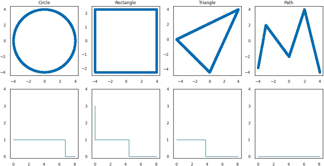
FIGURE 1. First row: a dense point cloud sampling without noise from each of the shapes. Second row: the corresponding standard stable ranks of the persistence modules given by the 1-st homology of the Vietoris-Rips complexes of the distances given by the restriction of the Euclidean metric to the point clouds.

3.2 Plane Figures: Analysis Based on Zero-th Homology

As a first exploratory step, for each plane figure we compute the Vietoris-Rips filtration, the corresponding 0-th homology persistence module and its stable rank with respect to the standard pseudometric. Figure 2 shows four plane figures with different labels from our dataset (first row) and the corresponding stable ranks (second row). By plotting the average of all stable ranks for plane figures corresponding to each shape (Figure 3) we get an indication that indeed the 0-th homology analysis may not be very effective at distinguishing between plane figures labeled by different shapes. To confirm this, we formulate our problem in machine learning terms as classifying a given plane figure to the shape from which it was generated. The dataset is split into a training set (70%) and a test set (30%). A support vector machine (SVM) is fitted on the training set using the standard stable rank kernel and evaluated on the test set. We take advantage of the fact that we can generate the data and repeat the whole procedure 20 times. This results in a rather weak average classification accuracy of 35.0%. We suspect that the poor classification is due to the fact that the plane figures do not exhibit distinct clustering patterns. The stable rank, with respect to the standard pseudometric, is a fully discriminatory invariant of persistence modules resulting from the 0-th homology of Vietoris-Rips filtrations (this is a consequence of the fact that the stable rank is a certain bar count, see Hierarchical Stabilization: From Persistence Modules to Measurable Functions). Since this invariant completely describes our 0-th homology persistence modules, we do not expect that the classification accuracy can be noticeably improved by considering stable rank kernels associated with different pseudometrics.

FIGURE 2

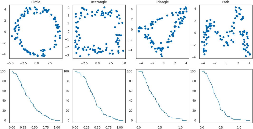
FIGURE 2. First row: examples of point clouds representing four plane figures in the dataset, one for each of the four shapes. Second row: the corresponding standard stable ranks of the persistence modules given by the 0-th homology of the Vietoris-Rips complexes of the plane figures.

FIGURE 3

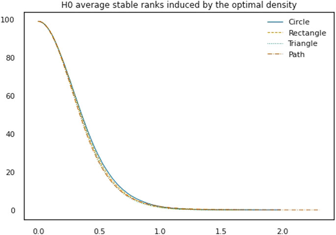
FIGURE 3. Average 0-th homology standard stable ranks for each shape.

3.3 Plane Figures: Analysis Based on First Homology

We repeat the same procedure for the 1-st homology persistence modules of the Vietoris-Rips filtrations. An indication that these stable ranks may be more effective at distinguishing between shapes is given by observing their average per shape, plotted in (Figure 4A) together with the standard deviation. This intuition is confirmed when considering the corresponding classification problem, in which we now achieve 88.5% accuracy. Note that in comparison to the stable ranks of the shapes (Figure 1, second row), adding noise and averaging has the effect that the stable ranks of plane figures (Figure 4A) are smoother, and decrease more gradually. When considering persistence modules resulting from the 1-st homology of Vietoris-Rips filtrations, the stable rank associated to the standard pseudometric is no longer a fully discriminatory invariant. Therefore, to improve accuracy it might be a viable strategy to consider alternatives to the standard pseudometric. To generate additional pseudometrics, we will use actions of distance type, which we recall can be defined by means of densities (see Hierarchical Stabilization: From Persistence Modules to Measurable Functions). In Figure 5, we illustrate the effect of changing densities.

FIGURE 4

FIGURE 4. (A): Average 1-st homology standard stable ranks for each shape (shaded area: standard deviation). (B): Example of a density considered optimal during one run of the procedure. (C): Average 1-st homology stable ranks with respect to the optimal pseudometric for each shape (shaded area: standard deviation).

FIGURE 5

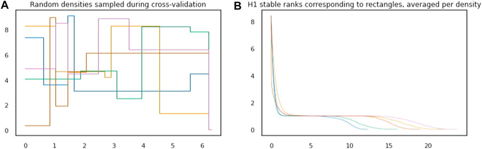
FIGURE 5. (A): Examples of five densities randomly sampled during cross-validation. (B): For plane figures in the dataset corresponding to the rectangle, stable ranks are computed under the five different densities from the left plot. Average stable ranks are plotted with the same color as the density under which they were computed.

As explained in Modeling: Determining Appropriate Distances on Persistence Modules, our strategy to produce densities is to restrict to a simple class of piecewise constant functions. We randomly sample 100 such densities and select the density corresponding to the optimal pseudometric using a cross-validation procedure. The density leading to the best accuracy on the validation set is kept and finally the accuracy on the test set is evaluated and reported.

Again because the dataset is artificially generated we can repeat the procedure many times to get robust results. It appears that although sampling densities introduces another source of randomness, restricting the densities to a simple family allows the improvement to be consistent and outperform the standard action every time. On average, we obtain an accuracy of 94.75%. In Figures 4B,C, a density considered optimal during one run of the procedure is shown, together with the stable ranks with respect to that density.

In this case, a simple interpretation for why this density leads to better accuracy might be found by inspecting the average 1-st homology Betti curve per shape. We recall that the 1-st homology Betti curve measures, for t in the filtration scale, the number of bars in a bar decomposition of the 1-st homology persistence module which contain t. Further, averages and standard deviations can be computed per shape. As shown in Figure 6 it appears that the rectangle and the triangle (which are the sources of confusion in the classification problem) are most easily distinguished by the 1-st homology Betti curve approximately in the interval [3, 4.5] of the filtration scale. Intuitively, the optimal density emphasizes this interval, leading to better accuracy. In particular the density with value one in the interval [3, 4.5] and value 0.05 elsewhere leads to comparable results as obtained by using an optimal density found through the cross-validation scheme.

FIGURE 6

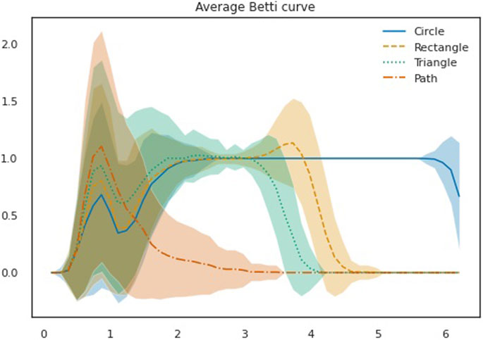
FIGURE 6. Average 1-st homology Betti curve for each shape (shaded area: standard deviation).

3.4 Plane Figures: Analysis Based on Subsampling, Averaging, and First Homology

We now modify our dataset. To add ambient noise to the point clouds we generate: 30% of the 100 points that constitute each point cloud are now sampled uniformly from the $\left[-\mathrm{5,5}]\times [-\mathrm{5,5}\right]$ square. The remaining 70% of the points are sampled as described before (see Plane Figures: Dataset Generation). In this way we obtain a new dataset of 2000 distance spaces labeled again by four shapes. Figure 7 shows four point clouds representing four plane figures with different labels in this new dataset. This figure also shows the corresponding standard stable ranks of the persistence modules given by the 1-st homology of the Vietoris-Rips complexes of the distances given by the restriction of the Euclidean metric to the point clouds. The addition of ambient noise has a substantial negative effect: patterns detected by persistent homology such as formation of clusters and voids are very sensitive to the insertion of even a small number of uniformly distributed points. This negative effect is well illustrated in Figure 8A where the average of 1-st homology standard stable ranks appear less distinctive for different shapes. However, a simple procedure of subsampling allows us to denoise the data, leading to an invariant which again can discriminate between the different shapes. For each point cloud, we now subsample 20% of its points and generate the corresponding 1-st homology standard stable rank. We repeat this 50 times and compute the average of these 50 stable ranks. Repeating this for all distance spaces in the dataset we obtain 2000 functions whose averages per shape are illustrated in Figure 8B. Using the same classification procedure as described in Plane Figures: Analysis Based on First Homology, we obtain a much higher shape detection accuracy of 86.25%.

FIGURE 7

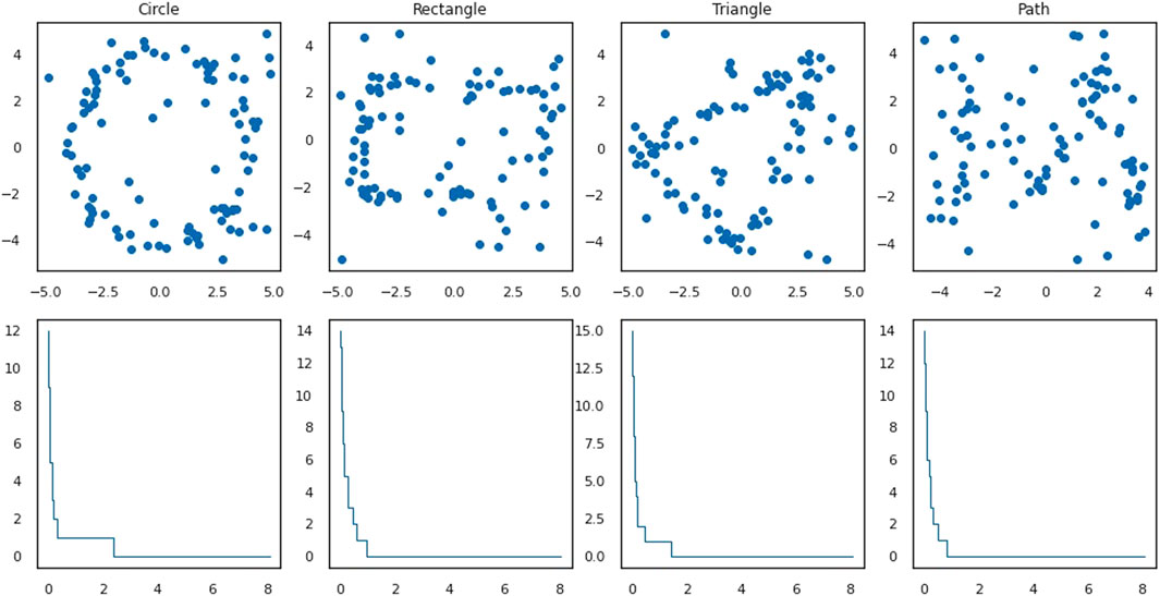
FIGURE 7. First row: examples of point clouds representing four plane figures in the dataset, one for each of the four shapes, with 30% ambient noise. Second row: the corresponding standard stable ranks of the persistence modules given by the 1-st homology of the Vietoris-Rips complexes of the plane figures.

FIGURE 8

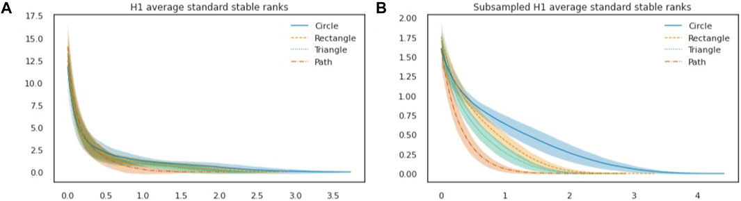
FIGURE 8. Point clouds generated with ambient noise. (A): 1-st homology average standard stable ranks (shaded area: standard deviation). (B): plane figures are represented by average 1-st homology standard stable ranks of subsamplings. Averages of these representations per shape are illustrated (shaded area: standard deviation).

Finally, instead of fixing the level of noise at 30% we now vary it by considering noise levels $0\text{\%},10\text{\%},20\text{\%},\dots ,90\text{\%},100\text{\%}$. For each noise level the same process is repeated: generation of figures, subsampling, generation of stable ranks, averaging, and classification, resulting in an accuracy for each level. This procedure was performed both with and without subsampling, as shown in Figure 9. As expected, the results are similar in accuracy when there is 0% noise and also when there is 100% noise. However, in between the subsampling clearly leads to an improvement.

FIGURE 9

FIGURE 9. For each level of ambient noise, classification is performed with standard stable ranks resulting from point clouds without subsampling (solid line) and with subsampling (dashed line) and classification accuracies are reported.

3.5 Activity Monitoring

As a real world dataset, we consider activity monitoring data from the PAMAP2 [20] dataset which consists of time series labeled per activity and per indivdual. On average, each time series has 13,872 time steps. The data was preprocessed as in [8]. We select two activities (ascending and descending stairs) and seven individuals. By taking the Cartesian product of activities and individuals we thus obtain 14 classes. For each class, which thus represents temporal measurements of one activity performed by one individual we remove the time steps that had no reported heart rate. We also remove a number of columns suspected to contain invalid information. That resulted in 28-dimensional time series with 1,268 time steps on average per individual and per activity. We then sample uniformly without replacement 100 time steps from each of these time series independently. Using the Euclidean distance we obtain a metric space (of size 100) per individual and per activity. Computing 0-th-and 1-st persistent homologies of the Vietoris-Rips filtrations of these metric spaces results in persistence modules. By repeating this procedure 100 times we obtain a dataset consisting of 1,400 observations (100 for each class) where each observation is a pair of persistence modules. Stable ranks can then be computed, first with respect to the standard action. In Figure 10 average standard stable ranks per class are plotted, both for 0-th and 1-st homologies. One can see that stable ranks allow to distinguish between individuals but even more so between activities.

FIGURE 10

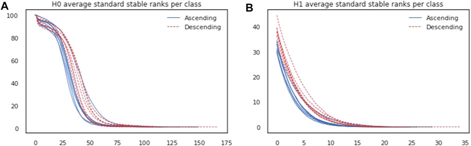
FIGURE 10. (A): 0-th homology average standard stable ranks per class. (B): 1-st average standard stable ranks per class.

The problem is formulated as classifying an out-of-sample pair of persistence modules within one of the 14 classes. In contrast with [8] but similarly to the previous experiment, we use an SVM classifier with the stable rank kernel. We construct two kernels, corresponding to 0-th and 1-st homologies respectively, using stable rank with respect to the standard action. For this experiment, however, both kernels appear to be informative and we wish to combine them to achieve better classification accuracy. Since a sum of kernels is also a kernel, we train our SVM with the sum of the kernels for the 0-th and 1-st homologies. There are also other ways to combine multiple kernels into a new one such as taking linear combinations or products [21], which might be useful for other experiments. We use random subsampling validation repeated 20 times with a $60/40$ training/test set split. This results in a 68.2% accuracy, demonstrating an improvement over [8] where 60% accuracy was obtained.

Next we apply the same procedure of cross-validation as in the previous experiment to attempt to find a better density and corresponding pseudometric and kernel. We search for alternative densities for the 1-st homology stable rank kernel while keeping the standard action for 0-th homology. This leads to an accuracy of 71.7%, thus somewhat higher than with the standard action. We note that the densities found through this method are similar to the one used in [8] which also led to an improvement. The confusion matrix corresponding to this kernel is shown in Figure 11.

FIGURE 11

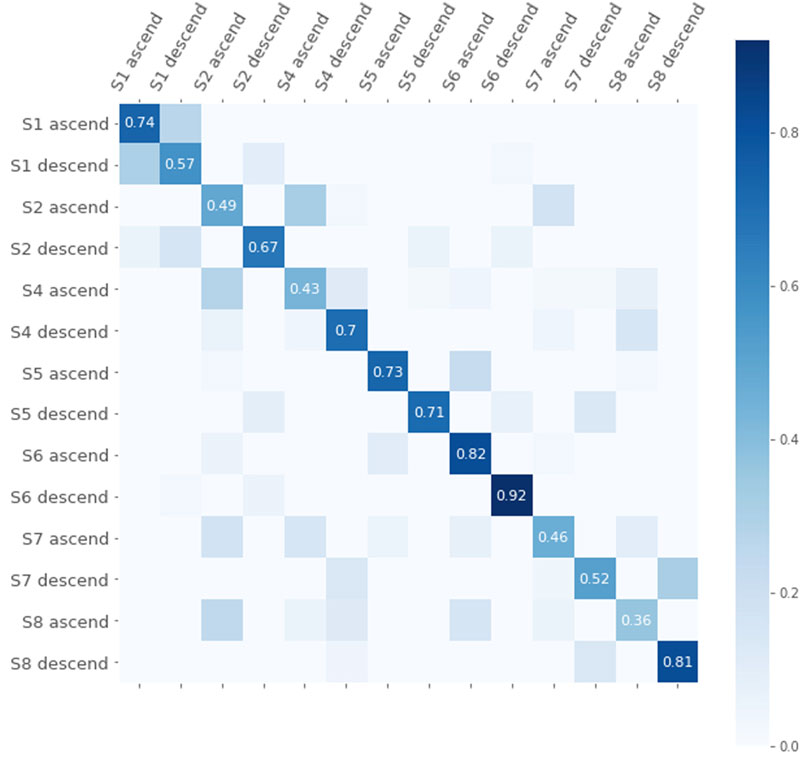
FIGURE 11. Confusion matrix for the classification with the kernel based on the 0-th homology standard stable rank and the 1-st homology stable rank with respect to the optimal density.

4 Discussion

A common pipeline when working with persistent homology is to start with a unique distance on persistence modules (Bottleneck or Wasserstein), then analyze persistence diagrams and finally consider feature maps from persistence diagrams, in case machine learning algorithms are to be applied. Our aim in this article has been to illustrate an alternative pipeline, where we instead start with a vast choice of distances on persistence modules and then consider the induced stable rank which is a continuous mapping with respect to the chosen distance. Our approach is very flexible, distances can be derived from parametrisations (densities) which often have an intuitive interpretation and can be found from simple search procedures, as we wanted to illustrate in the experiments. We believe that this simpler pipeline makes it natural to go between data analysis and machine learning, as stable ranks are amenable to both. For instance, we have presented how intuitions guided by the average of stable ranks then corresponded to classification accuracies through the stable rank kernel. Finally the simplicity of stable ranks makes them computationally efficient, something that is particularly useful for kernel methods.

A schematic situation where alternative distances can be useful, is when the bar decomposition of the classes is as follows. In the first, noisy, part of the filtration scale, bars are distributed randomly following the same distribution for both classes. In the second part of the filtration scale instead, bars are distributed according to two distinct distributions, one for each of the classes. Bottleneck distance is too sensitive to the noise, to utilize the signal, for instance in a classification problem. A distance defined by a density which has small values on the first part of the filtration scale and high values on the second part of the filtration scale, would instead extract the difference between the classes and result in a better classification when encoded in the stable rank kernel. In this case we could directly design a density which improves accuracy in a classification task. In other occasions, as we have shown for example in the plane figures dataset, Betti curves can give an indication of how to design appropriate densities. More generally, when the noise pattern becomes more complicated, we have proposed to randomly generate densities and then evaluate them in a cross-validation procedure. This method was particularly useful for the activity monitoring dataset, where given the difficulty of this classification problem, it was not possible to manually construct densities which improved classification. For the plane figure dataset instead we could still construct densities which perform as well if not slightly better than the optimal density among the randomly generated ones.

Learning algorithms for density optimization are an appealing alternative to this strategy, although we believe conceptual and algorithmic challenges are inherent to this problem. If for example density optimization is framed in terms of metric learning, the most difficult part is to identify a meaningful and well behaved objective function to optimize. Preliminary work by O. Gävfert [22], highlights that the choice of basic objective functions do not lead to convex optimization problems. Here we circumvent the question of identifying an appropriate objective function by evaluating the performance of a density through the accuracy of the associated kernel in SVM.

To enhance analysis using our methods one should keep in mind that in most cases it is convenient to consider several distances at the same time. For example different degree homologies (e.g., 0-th and 1-st homologies) could, and possibly should, be treated independently. In other words, distances that are suitable for the 0-th homology might not be informative for the 1-st homology. Even for analysis involving only one degree homology one should not look for just one density and one kernel since stable ranks with respect to different densities might show different geometrical aspects of the data. In principle it is possible to fully recover persistence modules, by using stable ranks (see Modeling: Determining Appropriate Distances on Persistence Modules and [8]), however in practice the whole information of the persistence modules might be redundant, while with an appropriate number and choice of densities, we believe, one could be able to extract more valuable information for a classification task.

While the examples in this article concern classification problems based on one-dimensional persistence, a more general treatment of the kernel would be interesting, both in terms of multi-persistence (the stable rank kernel is a multi-persistence kernel but the barcode decomposition in the one-dimensional case allows to compute it very efficiently), and in terms of utilizing the kernel in other contexts, such as for statistical inference.

Data Availability Statement

The original contributions presented in the study are included in the article/Supplementary Material, further inquiries can be directed to the corresponding author.

Author Contributions

This article is based on JA thesis [11]. JA, MS, WC, and RR conceived and developed the study. JA performed the data analyses. JA, MS, WC, and RR wrote the paper.

Funding

JA was partially supported by the Wallenberg AI, Autonomous Systems and Software Program (WASP) funded by Knut and Alice Wallenberg Foundation. WC was partially supported by VR, the Wallenberg AI, Autonomous System and Software Program (WASP) funded by Knut and Alice Wallenberg Foundation, and MultipleMS funded by the European Union under the Horizon 2020 program, grant agreement 733,161. RR was partially supported by MultipleMS funded by the European Union under the Horizon 2020 program, grant agreement 733,161. MS was partially supported by the Wallenberg AI, Autonomous Systems and Software Program (WASP) funded by Knut and Alice Wallenberg Foundation, VR, and Brummer and Partners MathDataLab. Support of the Wallenberg AI, Autonomous Systems and Software Program (WASP) funded by Knut and Alice Wallenberg Foundation was indispensable for conducting this research.

Conflict of Interest

The authors declare that the research was conducted in the absence of any commercial or financial relationships that could be construed as a potential conflict of interest.

References

1. Hausmann, JC. On the Vietoris-Rips Complexes and a Cohomology Theory for Metric Spaces. Prospects in Topology (Princeton, NJ, 1994) (Princeton Univ. Press, Princeton, NJ). Ann Math Stud (1995) 138:175–88. doi:10.1515/9781400882588-013

Google Scholar

2. Edelsbrunner, H, Letscher, D, and Zomorodian, A. Topological Persistence and Simplification. 41st Annual Symposium on Foundations of Computer Science (Redondo Beach, CA, 2000, Topological Persistence and Simplification). Los Alamitos, CA: IEEE Comput. Soc. Press (2000). p. 454–63. doi:10.1109/SFCS.2000.892133

CrossRef Full Text

3. Edelsbrunner, H, Letscher, D, and Zomorodian, A. Topological Persistence and Simplification. Discrete Comput Geom (2002) 28:511–33. doi:10.1007/s00454-002-2885-2

CrossRef Full Text | Google Scholar

4. Nielson, JL, Paquette, J, Liu, AW, Guandique, CF, Tovar, CA, Inoue, T, et al. Topological Data Analysis for Discovery in Preclinical Spinal Cord Injury and Traumatic Brain Injury. Nat Commun (2015) 6:8581. doi:10.1038/ncomms9581

PubMed Abstract | CrossRef Full Text | Google Scholar

5. Marian, G, and Yuri, K. Topological Data Analysis of Financial Time Series: Landscapes of Crashes. Physica A: Stat Mech its Appl (2018) 491:820–834. doi:10.1016/j.physa.2017.09.028

Google Scholar

6. Mileyko, Y, Mukherjee, S, and Harer, J. Probability Measures on the Space of Persistence Diagrams. Inverse Probl (2011) 27:124007. doi:10.1088/0266-5611/27/12/124007

CrossRef Full Text | Google Scholar

7. Turner, K, Mileyko, Y, Mukherjee, S, and Harer, J. Fréchet Means for Distributions of Persistence Diagrams. Discrete Comput Geom (2014) 52:44–70. doi:10.1007/s00454-014-9604-7

CrossRef Full Text | Google Scholar

8. Chachólski, W, and Riihimäki, H. Metrics and Stabilization in One Parameter Persistence. SIAM J Appl Algebra Geometry (2020) 4:69–98. doi:10.1137/19M1243932

CrossRef Full Text | Google Scholar

9. Oliver, G, and Wojciech, C. Stable Invariants for Multidimensional Persistence. arXiv [Preprint] (2017). Available from: https://arxiv.org/abs/1703.03632v1

Google Scholar

10. Scolamiero, M, Chachólski, W, Lundman, A, Ramanujam, R, and Öberg, S. Multidimensional Persistence and Noise. Found Comput Math (2017) 17:1367–406. doi:10.1007/s10208-016-9323-y

CrossRef Full Text | Google Scholar

11. Agerberg, J. Statistical Learning And Analysis On Homology-Based Features. Master’s Thesis. KTH Royal Institute of Technology, Stockholm (2020).

12. Reininghaus, J, Huber, S, Bauer, U, and Kwitt, R. A Stable Multi-Scale Kernel for Topological Machine Learning. Proc IEEE Conf Comput Vis pattern recognition (2015), 4741–4748. doi:10.1109/cvpr.2015.7299106

Google Scholar

13. Zhao, Q., and Wang, Y. (2019). “Learning Metrics for Persistence-Based Summaries and Applications for Graph Classification,” in Advances in Neural Information Processing Systems. Editors H. Wallach, H. Larochelle, and A. Beygelzimer (Red Hook, NY:Curran Associates, Inc.) 32.

Google Scholar

14. Massey, WS. A Basic Course in Algebraic Topology. Graduate Texts Mathematics (1991) 27:xvi+428. doi:10.1007/978-1-4939-9063-4

Google Scholar

15. Zomorodian, A, and Carlsson, G. Computing Persistent Homology. Discrete Comput Geom (2005) 33:249–74. doi:10.1007/s00454-004-1146-y

CrossRef Full Text | Google Scholar

16. Chazal, F, de Silva, V, Glisse, M, and Oudot, S. The Structure and Stability of Persistence Modules. Springer International Publishing (2016).

17. Anderson, I. Combinatorics of Finite Sets. Oxford Science Publications. New York: The Clarendon Press, Oxford University Press (1987). p. xvi+250.

18. Bauer, U. Ripser: Efficient Computation of Vietoris-Rips Persistence Barcodes. arXiv [Preprint] (2019). Available from: https://arxiv.org/abs/1908.02518v1

19. Chazal, F, Cohen-Steiner, D, Glisse, M, Guibas, LJ, and Oudot, SY. Proximity of Persistence Modules and Their Diagrams. In: Proceedings of the 25th Annual Symposium on Computational Geometry SCG ’09 (2009). p. 237–46.

Google Scholar

20. PAMAP, . Physical Activity Monitoring for Aging People. Available from: www.pamap.org.

21. Shawe-Taylor, J, and Cristianini, N, Kernel Methods for Pattern Analysis. Cambridge University Press, Cambridge (2004).

22. Gävfert, O. Topology-based Metric Learning (2018). Available from: https://people.kth.se/∼oliverg/