Collective Cell Migration in a Fibrous Environment: A Hybrid Multiscale Modelling Approach

Introduction

A large proportion of cancer research is currently focused on the role of tumour microenvironment on cancer progression, and in this context particular attention has been given to the interactions between the cancer cells and the extracellular matrix (ECM) and its components [1]. The ECM is composed of water, minerals, proteoglycans and fibrous proteins secreted by various cells, and these components appear in specific percentages in each organ in the body, according to the needs of the tissues [1]. Collagen is the most abundant fibrous protein in the ECM, and its importance is not only given by its role in the ECM architecture [1], but also by its role on tumour tissue stiffness, in promoting tumour metastasis and in the regulation of tumour immunity [2]. Different tissues have different levels of collagen [3]: from $\approx 75.4\mu g/$ mg tissue in pancreas, to $\approx 90\mu g/$ mg tissue in lung. Moreover, the orientation of collagen fibres plays a very important role in the mechanical properties of tissues, as well as in their physiological and biochemical functions [4]. In different tissues these fibres have different orientations addressing different functional needs [4, 5]: e.g., they are arranged in parallel in the tendons [5], or in concentric rings in the bone [6], or in orthogonal grids in the cornea [7] or hypertrophied myocardium [8].

Diseases can lead to a loss of orientation of collagen fibres as well, which adopt a more random distribution; this was observed, for example, in liver fibrosis [9], in heart diseases [8], or in denervated bones with reduced mechanical stress [6]. Cancer cells are also involved in the re-orientation of collagen fibres around tumours, by changing the typical tangled and disorganised collagen fibres that can be found within the stroma, towards thickened collagen fibres that are aligned perpendicularly to the boundary of the invading tumour [1, 10]. The density and orientation of collagen fibres inside the ECM plays an important role also in the evolution of cancer, as cancer cells not only move along collagen fibres [1, 10], but they also remodel the ECM through degradation [e.g., via matrix metalloproteases (MMPs)] and deposition of new matrix proteins [11], which interfere with cell-cell and cell-ECM adhesion, as well as cell polarity [1].

Despite all this wealth of information regarding the role of ECM in cancer progression, there is still a poor understanding of the roles of collagen fibre orientation on the individual and collective migration of cancer cells (and the non-local interactions between cells via these stiffened fibres), how the cells remodel the ECM, and how these complex cell-fibre interactions impact the overall tumour shape and invasion pattern. In a seminal paper, Friedl and Alexander [12] have reviewed the different mechanisms of individual and collective cancer cell migration: from single cells amoeboid and mesenchymal migration, to multicellular amoeboid and mesenchymal streaming, and various types of collective cell migration (clusters, strands, or files). Friedl and Alexander [12] also mentioned the spatially-expanding tumours that undergo growth and thus passively move by pushing the surrounding tissue. In contrast to the cancer cells that actively move in a collective manner along collagen fibres, the spatially-expanding tumours can be found within a capsule of ECM formed of aligned collagen fibres that are circularly disposed around this growing tumour. The different modes of migration are unstable and can change upon variations in cell-cell and cell-ECM adhesion [12].

While many studies [12] discuss the various types of invasion of tumour aggregations (as a result of single cell interactions with other cells or with the ECM), it is still not fully understood how cells perceive other cells further away (although it seems that they can mechanically sense and react to the presence of other cells up to 100 µm away [13]), and how this perception can impact the overall tumour shape. Moreover, it is still not fully understood how the various tissue types can impact the migration of tumour cells and tumour aggregations (as tumours can develop at the boundaries of different tissues with different characteristics).

The goal of this study is to investigate migration cell patterns in various tissues with different levels of ECM fibres and different alignment levels, as we vary: 1) cells sensing radius, 2) cell-cell and cell-ECM adhesion strengths, 3) the orientation of ECM fibres and the ratio of fibres to non-fibres ECM components, 4) the structure of the domain, with various tissue patches that have different fibre orientations. To this end, we consider a hybrid multi-scale modelling approach where cells are modeled as discrete entities while the ECM (with its two phases: fibrous and non-fibrous) is continuous. We show that this hybrid model can reproduce a variety of cell migration types (e.g., cluster, strand or files) as well as a variety of tumour shapes: circular, elongated or irregular (with finger-like protrusions). We also show that cell sensing radius has an impact on tumour shape and migration pattern only when the ratio of fibres to non-fibres ECM components is increased from lower to higher ratios. Finally, we show that the evolution of tumours that arise at the boundaries of different tissues with different fibre orientations is influenced by the directionality of these fibres.

The paper is structured as follows. In The Multi-Scale Hybrid Model section we describe the multi-scale hybrid model for cell-cell and cell-ECM interactions. In Results section we discuss variety of numerical simulations obtained with this model, as we vary the above mentioned parameters. We conclude in Summary and Discussion section with a summary and a discussion of the importance of these results.

The Multi-Scale Hybrid Model

There are two main types of models that are often used to capture the dynamics of tumour development, namely discrete and continuous models. Both have advantages and drawbacks over the other [14] and to minimise these disadvantages, recent extensive efforts have been made to combine these models into hybrid ones [15].

We employ here a hybrid modeling framework [15] that combines the off-lattice agent based model MultiCell-LF [16–18] to represent the cells, and a multi-scale continuous framework [19–23] to represent the microenvironment. To facilitate the description of this multi-scale hybrid model, let us first introduce some useful notations from both frameworks. The model is defined within a maximal tissue cube $Y\in {\mathrm{ℝ}}^d$ with $d=2$ and time interval $[0,T]$. The state of an arbitrary individual cell is described by $C_i\left(t\right)=\left\{X_i\left(t\right),C_i^{rad}\left(t\right),C_i^{age}\left(t\right),C_i^{mat},C_i^{neigh}\left(t\right)\right\}$, where ${\mathbf{X}}_i\left(t\right)$ denotes the position of the cell center, $C_i^{\text{rad}}\left(t\right)$ the cell radius, $C_i^{age}\left(t\right)$ the current cell age, $C_i^{\text{mat}}$ the cell maturation age (i.e., the age when the cell is ready for division which is assigned at birth and so it is independent of time) and $C_i^{\text{neigh}}\left(t\right)$ denotes the number of neighbouring cancer cells at time t. Here, $i\in \left\{1,\dots ,M\left(t\right)\right\}$ where $M\left(t\right)$ is the number of cancer cells at time $t\in [0,T]$.

To connect the discrete model to the continuous one, we first need to generate a cancer cell density by using the individual cell properties. For this, let us first observe that such density can be determined by using the fraction of unit space that is occupied by the cancer cells. Therefore, at any macro-scale spatio-temporal position $\left(x,t\right)\in Y\times [0,T]$ the density of the cancer cell population in a square neighbourhood $\mathbf{B}\left(x,{\gamma }_{\text{Δ}x}\right)$ is given by

$c\left(x,t\right):=\frac{1}{\lambda \left(\mathbf{B}\left(x,{\gamma }_{\text{Δ}x}\right)\right)}\cdot {\displaystyle \underset{\mathbf{B}\left(x,{\gamma }_{\text{Δ}x}\right)}{\int }{\mathrm{ℐ}}_P\left(z\right)dz},\text{with}P:=\left\{{\displaystyle \underset{i=1}{\overset{M\left(t\right)}{\cup }}{\mathbf{B}}_{\parallel \cdot {\parallel }_2}\left(X_i\left(t\right),C_i^{\text{rad}}\left(t\right)\right)}\right\}(1)$

where $\lambda (\cdot )$ is the Lebesgue measure in ${\mathrm{ℝ}}^d$, ${\mathrm{ℐ}}_{(\cdot )}(\cdot )$ is the usual indicator function, and ${\mathbf{B}}_{\parallel \cdot {\parallel }_2}(X_i\left(t\right),C_i^{\text{rad}}\left(t\right)):=\{z\in Y|\parallel X_i-z{\parallel }_2\le C_i^{\text{rad}}\}$ describes the spatial region occupied by the body of an individual cell $C_i$ within the neighbourhood $\mathbf{B}\left(x,{\gamma }_{\text{Δ}x}\right):=\left\{z\in Y|\parallel x-z{\parallel }_{\infty }\le {\gamma }_{\text{Δ}x}\right\}$ that is given by a $\parallel \cdot {\parallel }_{\infty }-$ball of an appropriately chosen radius ${\gamma }_{\text{Δ}x}>0$ (which is proportional to the spatial step-size of the discretised computational domain Y).

Besides the discrete cancer cell population, here, also we consider the dynamics of a continuous multi-scale two-phase ECM. Specifically, we consider a fibre ECM phase, accounting for all major fibres (for instance collagen and fibronectin) whose macro-scale density and spatial bias are denoted by $F\left(x,t\right)$ and ${\theta }_f\left(x,t\right)$, respectively (for further details see Fibre Representation and Fibre Rearrangement Process). On the other hand, the ECM also consist of several other macromolecules such as non-fibrous proteins (for example amyloid fibrils), minerals, various enzymes, proteoglycans and polysaccharides. Hence, to capture the ECM as a whole, we bundle the rest of these non-fibres ECM constituents (i.e., everything that is not considered to be fibrous proteins) into the second phase that we refer to as the non-fibre ECM phase and denote it by $l\left(x,t\right)$.

Finally, for compact notation we denote by $\rho \left(\mathbf{u}\right)$ the total space occupied at position x, i.e.,

$\rho \left(\mathbf{u}\right):=c\left(x,t\right)+F\left(x,t\right)+l\left(x,t\right),$

where u represents the global three-dimensional tumour vector

$\mathbf{u}:={\left(c\left(x,t\right),F\left(x,t\right),l\left(x,t\right)\right)}^{\mathrm{⊺}}.$

The MultiCell-LF Model

For each single cell in the MultiCell-LF (Multi-Cell Lattice-Free) model, several individually-regulated life processes are included, such as cell ageing, cell growth, cell division, cell-cell and cell-ECM interactions, and cell contact inhibition.

The Cell Cycle

The lifespan of each cell is traced with the current cell age $C_i^{\text{age}}\left(t\right)$ that progresses at the same rate as time, and cell maturation age $C_i^{\text{mat}}$ that is assigned at the cell birth and varies slightly between the cells to avoid synchronization of cell divisions. The cell cycle is divided into the usual four phases [24]: the G1 phase (gap 1) during which the cells are growing in size, the S phase (synthesis) when biological cells replicate their DNA, the G2 phase (gap 2) in which cells complete the growth and replication processes in preparation for the M phase (mitosis) in which cells physically divide into two daughter cells. Following ours and others previous work, the length of the cell cycle is divided as follows: G1 ($45\text{\%}$ of the whole cell cycle), S ($35\text{\%}$), G2 ($15\text{\%}$), and M ($5\text{\%}$), respectively [16, 17, 25]. Within the figures, we indicate the phase of an individual cell by different colours, i.e., we use white for the G1 phase, yellow for the S phase, orange for the G2 phase, red for the M phase and black for cells that are both in M phase and contact inhibited.

Cell Growth and Division

The radius $C_i^{\text{rad}}\left(t\right)$ of a growing cell is increasing linearly until it reaches the size of the mature cell $R_{max}$. The radius increment has been chosen to assure that the process of cell growth is completed before the M phase. Once the cell current age reaches its division age (i.e., $C_i^{\text{age}}\left(t\right)=C_i^{\text{mat}}$), it will divide into two daughter cells that are placed symmetrically around the mother cell’s nucleus ${\mathbf{X}}_i$ (t) within a distance equal to the half of the cell maximal radius [16, 17]:

${\mathbf{X}}_{i_1}\left(t\right)={\mathbf{X}}_i\left(t\right)+\frac{1}{2}{R}_{\text{max}}\left(\text{cos}\left(\varphi \right),\text{sin}\left(\varphi \right)\right),{\mathbf{X}}_{i_2}\left(t\right)={\mathbf{X}}_i\left(t\right)-\frac{1}{2}{R}_{\text{max}}\left(\text{cos}\left(\varphi \right),\text{sin}\left(\varphi \right)\right),(2)$

where ϕ is an angle randomly chosen from $\left[\mathrm{0,2}\pi \right]$, ${\mathbf{X}}_i\left(t\right)$ is the position of the mother cell, and $R_{\text{max}}$ is the maximal cell radius. The initial ages of the two new cells are set to zero ($C_{i_1}^{\text{age}}\left(t\right)=C_{i_2}^{\text{age}}\left(t\right)=0$), and their respective maturation ages $C_{i_1}^{\text{mat}}$ and $C_{i_2}^{\text{mat}}$ are inherited from the mother cell maturation age with a small noise term ${\mathit{ϵ}}_{\text{mat}}$ to avoid cell cycle synchronisation between the cells [17, 26]:

$C_{i_1}^{\text{mat}}=C_i^{\text{mat}}\left(1+{\mathit{ϵ}}_{\text{mat}}\right),C_{i_2}^{\text{mat}}=C_i^{\text{mat}}\left(1+{\mathit{ϵ}}_{\text{mat}}\right),$

where ${\mathit{ϵ}}_{\text{mat}}$ is a small number drawn from a uniform distribution $[-0.05,0.05]$ and $C_i^{\text{mat}}$ is the division age of the mother cell. Finally, both initial radii of the daughter cells are set to $0.65R_{\text{max}}$ (i.e., $C_{i1}^{\text{rad}}\left(t\right)=C_{i2}^{\text{rad}}\left(t\right)=0.65R_{\text{max}}$) and as a result initially the two daughter cells are overlapping Eq. 2. Therefore, right after the cell division, both daughter cells experience repulsive forces between each other, as well as with other nearby cells. These forces will push the cells apart until they reach an equilibrium and are no longer overlapping (see The Hybrid Cell Movement).

Cell Contact Inhibition

Once the whole cell colony grows in size, individual cells may become overcrowded and growth-arrested due to the contact inhibition signals from the neighbouring cells. The overcrowding condition is modelled by counting the number of cells $C_i^{neigh}\left(t\right)$ in the specified neighbourhood of radius $R_{neigh}=4.5R_{\max }$:

$C_i^{\text{neigh}}\left(t\right)={\displaystyle \sum }_{j=1}^{M\left(t\right)}{\mathrm{ℐ}}_{S{S}_i}\left({\mathbf{X}}_j\left(t\right)\right),$

where ${\mathrm{ℐ}}_{(\cdot )}(\cdot )$ again denotes the indicator function and $S{S}_i$ is the set of all cancer cells that are close to the cell $C_i\left(t\right)$, i.e.,

$S{S}_i=\left\{\mathbf{X}\in {\left\{{\mathbf{X}}_k\left(t\right)\right\}}_{k=1,\dots ,M\left(t\right)}|{\Vert \mathbf{X}-{\mathbf{X}}_i\left(t\right)\Vert }_2\le R_{\text{neigh}}\right\}\backslash \left\{{\mathbf{X}}_i\left(t\right)\right\}.$

When the number of neighbouring cells reaches a specified threshold $N_{\text{neigh}}$ (i.e., $C_i^{\text{neigh}}\left(t\right)\ge N_{\text{neigh}}$), the cell $C_i$ (t) is considered overcrowded and growth-arrested. However, such an arrested cell remains metabolically active [27], and can resume its active cell cycle when the contact inhibition conditions change. The time spent in the growth-arrested state does count toward the length of the active cell cycle.

The Hybrid Cell Movement

To model cancer cell passive relocation (due to cell-cell interactions) and active migration (due to cell-ECM interactions), we combine both discrete and continuous approaches. While for cell-cell interactions (both repulsive and adhesive forces) we use the agent-based approach, the cell- ECM (both fibre-based and non-fibre adhesions) are modelled by using a continuous technique. Ultimately, these forces collectively influence the direction of motion of each individual cell, leading to complex tumour dynamics and to the emergence of various tumour morphologies.

Discrete Cell-Cell Repulsive Interactions

The repulsive forces between nearby cells are introduced to maintain cell volume and to avoid cell overlapping during its movement or division (see Cell Growth and Division). Following our previous work [17, 18], these forces are modelled as linear Hookean springs. Hence, considering two arbitrary but distinct cells $C_i\left(t\right)$ and $C_j\left(t\right)$ (with $i\ne j$), the repulsive force between them is given by:

${\mathbf{F}}_{i,j}^{\text{rep}}=\{\begin{array}{cc}{F}^{\text{rep}}\left(\left(C_i^{\text{rad}}\left(t\right)+C_j^{\text{rad}}\left(t\right)\right)-{\Vert {\mathbf{X}}_i\left(t\right)-{\mathbf{X}}_j\left(t\right)\Vert }_2\right)\frac{{\mathbf{X}}_i\left(t\right)-{\mathbf{X}}_j\left(t\right)}{{\Vert {\mathbf{X}}_i\left(t\right)-{\mathbf{X}}_j\left(t\right)\Vert }_2},& \text{if}{\Vert {\mathbf{X}}_i\left(t\right)-{\mathbf{X}}_j\left(t\right)\Vert }_2<C_i^{\text{rad}}\left(t\right)+C_j^{\text{rad}}\left(t\right),\\ 0,& \text{otherwise},\end{array}$

where $F^{\text{rep}}>0$ is the constant spring stiffness and the spring resting length is set be equal to the sum of the two cells’ radii, i.e., to $C_i^{\text{rad}}\left(t\right)+C_j^{\text{rad}}\left(t\right)$. Taking into consideration now the whole cancer cell population, the overall repulsive force that acts on the cell $C_i\left(t\right)$ is given by the sum of all repulsive forces between the cell $C_i\left(t\right)$ and any other overlapping cell $C_j\left(t\right)$, with $j\in \left\{1,\dots ,M\left(t\right)\right\}\backslash \left\{i\right\}$. This cumulative force is given by

${\mathrm{ℱ}}_i^{\mathrm{r}\mathrm{e}\mathrm{p}}:={\displaystyle \sum }_j{F}_{i,j}^{\mathrm{r}\mathrm{e}\mathrm{p}},j\in \left\{1,\dots ,M\left(t\right)\right\}\backslash \left\{i\right\}.(3)$

Discrete Cell-Cell Adhesive Interactions

The adhesive forces are activated between non-overlapping but nearby cells in order to keep the cell cluster compact. These forces are modelled using Hooke’s law with a constant spring stiffness $F^{\text{adh}}>0$ and resting length of 2 $R_{\text{max}}$[17]. Hence, such forces are activated between cells separated by the distance larger than $2R_{\max }$, but not exceeding $2.25R_{\text{max}}$. This prevents from over-activation of the cell-cell adhesion between cells that are located far off each other. Therefore, considering two arbitrary cells $C_i\left(t\right)$ and $C_j\left(t\right)$ (with $i\ne j$), the cell-cell adhesion force acting between them is given by

${\mathbf{F}}_{i,j}^{\text{adh}}:=\{\begin{array}{cc}{F}^{\text{adh}}\left(2R_{\text{max}}-{\Vert {\mathbf{X}}_i\left(t\right)-{\mathbf{X}}_j\left(t\right)\Vert }_2\right)\frac{{\mathbf{X}}_i\left(t\right)-{\mathbf{X}}_j\left(t\right)}{{\Vert {\mathbf{X}}_i\left(t\right)-{\mathbf{X}}_j\left(t\right)\Vert }_2},& \text{if\hspace{0.17em}}{\Vert {\mathbf{X}}_i\left(t\right)-{\mathbf{X}}_j\left(t\right)\Vert }_2\in \left(2R_{\text{max}},2.25R_{\text{max}}\right)\\ 0,& \text{otherwise}.\end{array}$

Similarly to the repulsive forces, each cell can be subjected to multiple adhesive forces, thus the cumulative adhesive force which acts on cell $C_i\left(t\right)$ is given by

${\mathrm{ℱ}}_i^{\text{adh}}:={\displaystyle \sum _j{\mathbf{F}}_{i,j}^{\text{adh}}},j\in \left\{1,\dots ,M\left(t\right)\right\}\mathrm{\setminus }\left\{i\right\}.(4)$

Continuous Cell-ECM Adhesive Interactions

Besides the cell-cell interactions described above, of particular importance, are the cell-ECM adhesions [28–31] that we explore here through a cell-non-fibre ECM adhesion [32–35] as well as a cell-fibre ECM adhesion [36, 37]. In the existing literature [19–23, 38–42], this type of interaction is usually modelled by a non-local adhesion integral with a sensing region$B\left(0,R\right)$ of radius R. Since in our hybrid model the two phase ECM is modelled in a continuous manner using densities, we can adopt this approach to describe the present cell-ECM interactions. To this end, let us define the cell-ECM adhesion force/velocity for an arbitrary cell $C_i$ as

${\mathrm{ℱ}}_i^{\text{ECM}}:=\frac{1}{R}\underset{\mathbf{B}\left(0,R\right)}{{\displaystyle \int }}\mathcal{K}\left({\left|\left|y\right|\right|}_2\right)[n\left(y\right){\mathbf{S}}_{cl}l\left(X_i+y,t\right)+\widehat{n}\left(y,{\theta }_f\left(X_i+y,t\right)\right){\mathbf{S}}_{cF}F\left(X_i+y,t\right)]\cdot {[1-\rho \left(\mathbf{u}\right)]}^{+}dy,(5)$

where R represents the maximum range within which a cell $C_i$ can establish adhesive bonds with the surrounding ECM constituents, i.e., within $B\left(0,R\right)$ and $S_{cl}>0$ and $S_{cF}>0$ are assumed to be the constant cell-non-fibre ECM and cell-fibre ECM adhesion strengths, respectively. Furthermore, in Eq. 5 $n(\cdot )$ is the unit radial vector

$n\left(y\right):=\{\begin{array}{l}\frac{y}{{\left|\left|y\right|\right|}_2}\text{if }y\in \mathbf{B}\left(0,R\right)\mathrm{\setminus }\left\{0\right\},\\ 0\text{if }y=0.\end{array}$

and similarly $\widehat{n}(\cdot ,\cdot )$ is the unit radial vector biased by the orientation of the fibres, i.e., it is given by

$\widehat{n}\left(y,{\theta }_f\right):=\{\begin{array}{l}\frac{y+{\theta }_f\left(x+y,t\right)}{||y+{\theta }_f{\left(x+y,t\right)||}_2}\text{if }y\in \mathbf{B}\left(0,R\right)\mathrm{\setminus }\left\{0\right\},\\ 0\text{if }y=0,\end{array}$

where ${\theta }_f\left(x,t\right)$ is the macro-scale orientation of the fibres. For further details about the fibre orientations see Fibre Representation section. Also, in Eq. 5 to account for the gradual weakening of these adhesive bonds as we move away from the centre of the cell $X_i$ within the sensing region $B\left(0,R\right)$, we simply use a radially symmetric kernel $\mathcal{K}(\cdot )$ which is given by

$\mathcal{K}\left(y\right)=\psi \left(\frac{y}{R}\right),\forall y\in \mathbf{B}\left(0,R\right),$

where $\psi (\cdot )$ is the standard mollifier defined as

$\psi \left(x\right):=\{\begin{array}{cc}\frac{\text{exp}\left(\frac{-1}{1-||x{||}_2^2}\right)}{{\displaystyle \underset{\mathbf{B}\left(\mathrm{0,1}\right)}{\int }\text{exp}\left(\frac{-1}{1-||y{||}_2^2}\right)dz}}& \text{if }x\in \mathbf{B}\left(\mathrm{0,1}\right),\\ 0& \text{if }x\notin \mathbf{B}\left(\mathrm{0,1}\right).\end{array}$

Finally, in Eq. 5 ${[1-\rho \left(\mathbf{u}\right)]}^{+}:=\max \left(\mathrm{0,1}-\rho \left(\mathbf{u}\right)\right)$ ensures that any overcrowded space within the sensing region $B\left(0,R\right)$ does not influence the overall cell-ECM adhesion.

For completeness, here we also briefly discuss the numerical approach for the cell-ECM adhesion integral ${\mathrm{ℱ}}_i^{ECM}$ given in Eq. 5. To this end, we adopt the partitioning of the sensing region $B\left(0,R\right)$ from Shuttleworth and Trucu [19], and so we divide $B\left(0,R\right)$ into $N_s$ annulus sectors shown in Figures 1C,D.

FIGURE 1

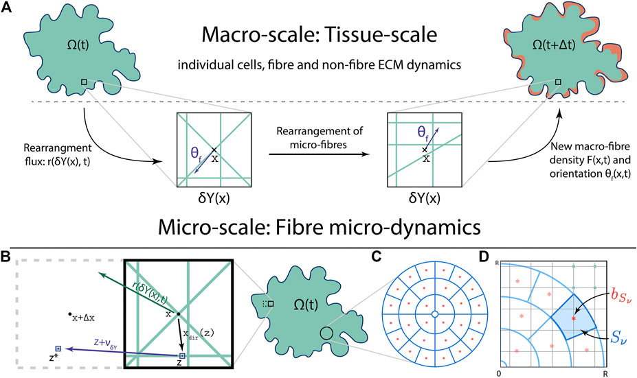
FIGURE 1. (A) Schematics of the multi-scale fibre dynamics, including the bottom-up and top-down links between the macro-scale and the fibre micro-scale (with: the green lines within $\delta Y\left(x\right)$ portraying the micro-distribution of micro-fibres; and the orange shaded area on the right tumour macro-domain representing the net cancer progression with respect to the previous time-step). (B) Schematic of the reallocation of the micro-fibre at position z to its new position $z^{\ast }$ which located in a neighbouring micro-domain $\delta Y\left(x+\Delta x\right)$. (C) Partitioning of the sensing region $B\left(0,R\right)$ into $N_s$ annulus sectors $S_{\nu }$ with barycentres $b_{S_{\nu }}$ (red stars). (D) Illustration of the top-right quarter of (C) overlaid on top of the macroscopic background mesh (grey grid). Here, we highlight an annulus sector $S_{\nu }$ (blue highlighted area), its corresponding off-grid barycentre $b_{S_{\nu }}$ (red star) and four of its macro-nodes (green dots).

Thus, as shown in Figure 1C, the sensing region $B\left(0,R\right)$ is split into s annuli and then each of these annuli is further split into $2^{m+\left(k-1\right)}$ uniformly distributed sectors, i.e., the number of annulus sectors is given by

$N_s:={\displaystyle \sum }_{k=1}^s{2}^{m+\left(k-1\right)}.$

Further, let us now denote these annulus sectors by $S_{\nu }$, with $\nu =1,\dots ,N_s$, and their corresponding off-grid barycentres by $b_{S_{\nu }}$, as shown in Figure 1D. Then, by using simple bi-linear shape functions, on each annulus sector $S_{\nu }$ we are able to approximate the mean-values of the non-fibres ECM, the fibres ECM, as well as their associated macro-scale orientations. Ultimately, this enables us to appropriately construct the integral of the step functions associated with each annulus sector $S_{\nu }$ whose value is given by a linear combination of the mean-values. Finally, these mean values are used to obtain the numerical approximation for ${\mathrm{ℱ}}_i^{ECM}$ by following the numerical steps described in full in [19, 22, 23].

The Overall Direction of Cell Movement

Ultimately, the overall movement direction of a cell $C_i\left(t\right)$ depends on each of the forces discussed above (repulsion, cell-cell adhesion and cell-ECM adhesion). To this end, the spatial dynamics of a cell $C_i\left(t\right)$ is based on Newton’s second law of motion where we assume that each cell returns to its equilibrium without oscillations. Further, the overall force acting on a cell $C_i\left(t\right)$ is assumed to be proportional to the velocity of the cell and so the dynamics is given by [16–18].

$\eta \frac{d{X}_i}{dt}={\mathrm{ℱ}}_i^{\text{rep}}+{\mathrm{ℱ}}_i^{\text{adh}}+{\mathrm{ℱ}}_i^{\text{ECM}},(6)$

where η is the damping coefficient and ${\mathrm{ℱ}}_i^{\text{rep}}$, ${\mathrm{ℱ}}_i^{\text{adh}}$ and ${\mathrm{ℱ}}_i^{\text{ECM}}$ are defined in Eqs 3–5, respectively. To solve the spatial dynamics Eq. 6 of the cell $C_i\left(t\right)$, we use the classical forward Euler method. We illustrate the overall travelling direction of a cell in Figure 2.

FIGURE 2

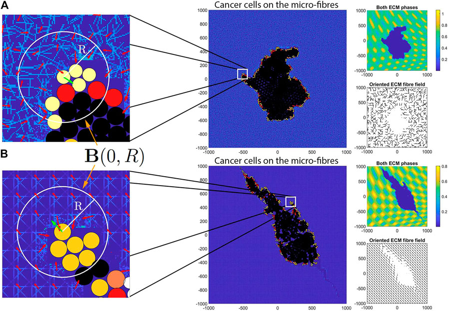
FIGURE 2. Illustration of the sensing region $B\left(0,R\right)$ of radius R around a cancer cell, highlighted by the white circle. Within the zoomed-in areas (on the left), the red arrows show the oriented ECM fibre field and the green arrow on the central cancer cell shows the overall travelling direction of that particular cancer cell which is the solution of Eq. 6. On the right, we show the individual cancer cells with the micro-fibres, the non-fibre ECM densities and the oriented ECM fibre fields (for illustrative purposes these are coarsened four-fold). (A) Cancer cell placed within a random fibre environment, identical to Figure 7C. (B) Cancer cell placed within an aligned fibre environment, identical to Figure 7A′.

The Continuous Multi-Scale ECM

Tumour development is a complex and multi-scale phenomena where the macro-scale events are accompanied by several related micro-scale processes. One of the most important of these processes is the re-distribution of the fibres ECM micro-constituents triggered by various cell-generated forces. Hence, here we first describe the macro-scale dynamics of the continuous two-phase ECM and then we detail its micro-scale dynamics.

Similarly to the cancer cell density, to achieve connection between the discrete and continuous parts of the model, we first need to appropriately approximate the generated cell forces (${\mathrm{ℱ}}_i^{rep}$, ${\mathrm{ℱ}}_i^{\text{adh}}$ and ${\mathrm{ℱ}}_i^{ECM}$ defined in Eqs 3–5, respectively) on the macro-scale. For this, let us use the average of the collective contribution of all cell generated forces within a ${\gamma }_{\text{Δ}x}$ neighbourhood of the macro-node x. This leads to the following continuous cancer cell flux:

$\mathrm{ℱ}\left(x,t\right):=\frac{{\displaystyle \underset{\mathbf{B}\left(x,{\gamma }_{\text{Δ}x}\right)}{\int }{\displaystyle \sum _{X_i\in \mathbf{B}\left(x,{\gamma }_{\text{Δ}x}\right)}\left({\mathrm{ℱ}}_i^{\text{rep}}+{\mathrm{ℱ}}_i^{\text{adh}}+{\mathrm{ℱ}}_i^{\text{ECM}}\right)\cdot {\mathrm{ℐ}}_{\mathbf{B}\left(X_i,C_i^{\text{rad}}\right)}\left(z\right)dz}}}{\lambda \left(\mathbf{B}\left(x,{\gamma }_{\text{Δ}x}\right)\right)\cdot {\displaystyle \sum _{i=1}^{M\left(t\right)}{\mathrm{ℐ}}_{\mathbf{B}\left(x,{\gamma }_{\text{Δ}x}\right)}}\left(X_i\right)},(7)$

where again $\lambda (\cdot )$ is the Lebesgue measure in ${ℝ}^d$, $B\left(x,{\gamma }_{\Delta x}\right)$ is the $\parallel \cdot {\parallel }_{\infty }$ ball used also in Eq. 1, ${\mathrm{ℐ}}_{(\cdot )}(\cdot )$ denotes the indicator function.

The Two-phase ECM

Besides the cancer cells, in this work we also take into account the dynamics of a two-phase ECM to capture not only the fibrous proteins in the fibres ECM, but also every other ECM constituents which are collected into the non-fibre ECM phase. It is well-known that MMPs are responsible for degrading the fibrous ECM proteins [43, 44], and since cancer cell do produce several types of MMPs [45, 46], here we consider the fibres ECM to be degraded by the cancer cell population at a constant rate ${\beta }_F>0$. However, existing biological evidence also suggest that besides the fibrous proteins, components of the non-fibre ECM phase can also be degraded by several classes of MMPs (for instance amyloid fibrils [47, 48]). Hence, we can assume a constant non-fibre ECM degradation rate ${\beta }_l>0$ by the cancer cells. The non-dimensional macro-scale dynamics of both fibre and non-fibre ECM phases are mathematically formalised as

$\frac{\partial F}{\partial t}=-{\beta }_{F}cF,\frac{\partial l}{\partial t}=-{\beta }_{l}cl.(8)$

Here, we used the macro-scale density of the cancer cell population $c\left(x,t\right)$ (see Eq. 1), which was derived using the properties of the individual cells provided by the agent-based part of our hybrid model.

Fibre Representation

Let us now focus our attention to the two macro-scale representations of the fibres ECM, namely its amount $F\left(x,t\right)$ and spatial bias ${\theta }_f\left(x,t\right)$. Considering a micro-scale distribution of the micro-fibres $f\left(z,t\right)$ on a cell-scale micro-domain $\delta Y\left(x\right):=x+\delta Y$ of appropriate micro-scale size $\delta >0$, we observe that both of these two characteristics of the fibres ECM can be captured through a vector field representation ${\theta }_f\left(x,t\right)$ of the fibres. This captures the naturally emerging macro-scale orientation of the ECM fibres that is induced by the distribution of micro-fibres constituents $f\left(z,t\right)$ at micro-scale (on $\delta Y\left(x\right)$), and represents the spatial bias of the ECM fibres distributed at x to withstand incoming spatial cell fluxes generated by the collective cell migration. Following Shuttleworth and Trucu [19], this vector field representation of the ECM fibre phase is given by

${\theta }_f\left(x,t\right):=\frac{1}{\lambda \left(\delta Y\left(x\right)\right)}\underset{\delta Y\left(x\right)}{{\displaystyle \int }}f\left(z,t\right)dz\cdot \frac{{\theta }_{x,\delta Y\left(x\right)}\left(x,t\right)}{||{\theta }_{x,\delta Y\left(x\right)}{\left(x,t\right)||}_2},$

where ${\theta }_{x,\delta Y\left(x\right)}\left(x,t\right)$ is the Bochner-mean-value [49] of the vector-valued function $\delta Y\left(x\right)\mathrm{\ni }z\mapsto z-x\in {\mathrm{ℝ}}^d$ with respect to the measure $f\left(z,t\right)\lambda (\cdot )$ and represents the uniquely emerging revolving barycentral orientation (which was originally derived and justified in detail in Shuttleworth and Trucu [19]) induced by the micro-fibre distribution $f\left(z,t\right)$ on $\delta Y\left(x\right)$, this being given by

${\theta }_{f,\delta Y\left(x\right)}\left(x,t\right):=\frac{{{\displaystyle \int }}_{\delta Y\left(x\right)}f\left(z,t\right)\left(z-x\right)dz}{{{\displaystyle \int }}_{\delta Y\left(x\right)}f\left(z,t\right)dz}.(9)$

In this context, the second characteristic of the fibres ECM, i.e., its amount $F\left(x,t\right)$ is precisely given by the Euclidean norm of the vector field ${\theta }_f\left(x,t\right)$, namely

$F\left(x,t\right):=||{\theta }_f{\left(x,t\right)||}_2,$

which in fact represents the mean-value of the micro-fibre distribution on the micro-domain $\delta Y\left(x\right)$. Since both of these macro-scale fibre ECM representations are derived by using the micro-scale distribution of the micro-fibres $f\left(z,t\right)$, there is an emerging link between the two scales which we refer to as the fibre bottom-up link and illustrate it in Figure 1A. Furthermore, the detailed micro-scale rearrangement process is illustrated in full in Figure 1B.

Fibre Rearrangement Process

As the individual cancer cells move and invade, they interact with the micro-fibre structure and thereby push them in the direction of travelling, ultimately resulting in the rearrangement of the micro-fibres. Following Shuttleworth and Trucu [19], here we consider this complex process to be initiated by the spatial flux of the cancer cell population $\mathrm{ℱ}\left(x,t\right)$ that was defined in Eq. 7. Then, such flux that acts uniformly on $\delta Y\left(x\right)$ naturally gets regulated in a weighted manner by the orientation of the fibres ${\theta }_f\left(x,t\right)$, resulting in a micro-fibres rearrangement vector

$r\left(\delta Y\left(x\right),t\right):=\omega \left(x,t\right)\mathrm{ℱ}\left(x,t\right)+\left(1-\omega \left(x,t\right)\right){\theta }_f\left(x,t\right),(10)$

where the weight $\omega \left(x,t\right)$ is the appropriate mass fraction of the cancer cells and fibres ECM given by

$\omega \left(x,t\right):=\frac{c\left(x,t\right)}{c\left(x,t\right)+F\left(x,t\right)}.$

Ultimately, the new position $z\text{*}$ of each micro-fibre $z\in \delta Y\left(x\right)$ is calculated by using a reallocation vector${\nu }_{\delta Y\left(x\right)}\left(z,t\right)$ which accounts not only for the rearrangement vector $r\left(\delta Y\left(x\right),t\right)$ in Eq. 10 but also upon the degree of alignment between $r\left(\delta Y\left(x\right),t\right)$ and the barycentral position vector$x_{dir}\left(z\right):=z-x$ as well as it utilises the level of micro-fibres at position z. Hence, this reallocation vector is given by

$\nu \delta Y\left(x\right)\left(z,t\right):=[x_{dir}\left(x\right)+r\left(\delta Y\left(x\right),t\right)]\cdot \frac{f\left(z,t\right)[f_{max}-f\left(z,t\right)]}{f\text{*}+{\left|\left|\mathit{r}\left(\delta Y\left(\mathit{x}\right),\mathit{t}\right)-x_{dir}\left(\mathit{x}\right)\right|\right|}_2}\cdot {\chi }_{\{f(z,t)>0\}},(11)$

where $f_{\max }>0$ is the maximum possible level of fibres at any micro-point z, $f^{\ast }:=f\left(z,t\right)/f_{\max }$ is the fibres saturation level and ${\chi }_{\{f(z,t)>0\}}$ is the characteristic function of the micro-fibres support. Therefore, by using Eq. 11 the new position $z\text{*}$ is given by

$\mathit{z}\text{*}:=z+{\nu }_{\delta Y\left(x\right)}\left(z,t\right),$

and the amount of fibres that is reallocated from z to $z\text{*}$ is determined by a movement probability

$p_{move}:=\text{max}\left(\mathrm{0,1}-\frac{f\left(z\text{*},t\right)}{f_{max}}\right),$

which tracks the free space available at the new position $z\text{*}$. Thus, the level of fibres that gets moved to $z\text{*}$ is given by $p_{move}\cdot f\left(z,t\right)$ and the rest of the fibres, i.e., $\left(1-p_{move}\right)\cdot f\left(z,t\right)$ remain at the current position z. In Figure 1B we illustrate the reallocation of a micro-fibre using a typical example of the rearrangement $r\left(\delta Y\left(x\right),t\right)$ and reallocation vectors ${\nu }_{\delta Y\left(x\right)}\left(z,t\right)$ defined in Eqs. 10, 11, respectively.

Finally, since this rearrangement process that redistributes the fibres ECM micro constituents is initiated by the macro-scale cancer cell flux $\mathrm{ℱ}\left(x,t\right)$, the macro and micro-scales are connected via a top-down link which is also illustrated in Figure 1A.

For a diagrammatic description of the full hybrid model, with the exact stages where the agent-based model of the cells connects with the continuous model of the ECM, please see Figure 15 in Appendix B.

Results

In the context of the above described multi-scale hybrid framework, here we present some numerical simulations of the model, which highlight different migration cell patterns in various tissues with different levels of ECM fibres and different alignment levels. To this end, we start each simulation with a single cancer cell with well defined properties located at a point $\left(x_1^0,x_2^0\right)$ (that will be defined for each simulations) of the computational domain $Y=[-1280mm,1280mm]\times [-1280mm,1280mm]$, and any alteration from this will be stated accordingly. Then, this single cancer cell is considered to be embedded within the following (scaled) non-fibre ECM environment [19–23]:

$l(x,0):=\frac{1}{2}+\frac{1}{4}\text{ sin }{\left(7\pi \frac{\left(x_1+1280\right)}{640}\frac{\left(x_2+1280\right)}{640}\right)}^3\cdot \text{sin}\left(7\pi \frac{x_2+1280}{x_1+1280}\right),$

which can be seen in Figure 3A that is in-silico representation of the heterogeneous distribution of the non-fibre ECM. For illustrative purposes, in Figure 3 (as well as throughout the rest of this Section) we present the non-fibre ECM initial conditions only on the domain of $[-1000mm,1000mm]\times [-1000mm,1000mm]$. Moreover, for both Figures 3A,B (as well as for all other figures in this Section), the units of the x and y axes are in ‘mm’. Finally to highlight the phase of each individual cell, we use five colours. Specifically, we colour the cells that are in the G1 phase white, those in the S phase yellow, those in the G2 phase orange, those in M phase red, and the ones that are both growth-arrested (due to contact inhibition) and in the M phase are coloured black in all simulations.

FIGURE 3

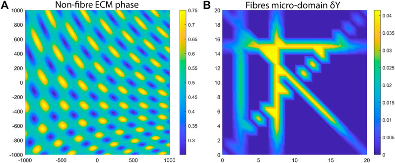
FIGURE 3. Initial ECM conditions used for the numerical simulations. (A) The macro-scale non-fibres ECM density. (B) One aligned micro-fibres domain $\delta Y$ which is repeated for all macro-node x.

To shed some light on the importance of ECM characteristics on cancer invasion, throughout this section we investigate numerically the type of cancer migration and invasion patterns obtained when we consider different cell sensing radii. We note here that the sensing radius is determined not only by the length of cell membrane protrusions called pseudopodia (which have lengths greater than 2 µm [50, 51]), but also by the long-range cell sensing due to stress transmission via aligned ECM fibres (which allows cells to sense other cells up to 100 µm away [13]). Throughout this study we investigate the impact of two sensing radii, $R=30\mu m$ or $R=50\mu m$, on tumour shape and invasion pattern. We also investigate the impact of different fibres to non-fibres ECM ratios (i.e., 10: 90%, 20: 80%, or 30: 70%), different ECM fibre distribution (i.e., random, aligned, or mixed), and different cell-cell and cell-ECM interaction strengths.

Simulations Without Cell-ECM Adhesions in a Random Fibrous Environment

We start our numerical investigation of this hybrid multi-scale model by showing some baseline simulations for the case without cell-ECM adhesions, as we vary the fibre ECM density (i.e., $10-30\text{\%}$ fibres), for two different sensing radii: $R=30\mu m$ in Figure 4, and $R=50\mu m$ in Figure 5.

FIGURE 4

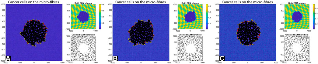
FIGURE 4. Simulation results at final time T = 28 days with random fibres, sensing radius $R=30\mu m$, repulsion $F^{rep}=0.45\times 10mg/\mu m\cdot {\min }^2$, cell-cell adhesion $F^{\text{adh}}=0.12\times 10mg/\mu m\cdot mi{n}^2$, cell-non-fibre ECM adhesion $S_{cl}=0$, cell-fibre ECM adhesion $S_{cF}=0$ and with (A) $10\%:90\%$, (B) $20\%:80\%$, (C) $30\%:70\%$ fibres and non-fibres ECM ratios. For illustrative purposes, all oriented ECM fibre fields are coarsened four-fold. Initial cell position was: (A–C) (0,0).

FIGURE 5

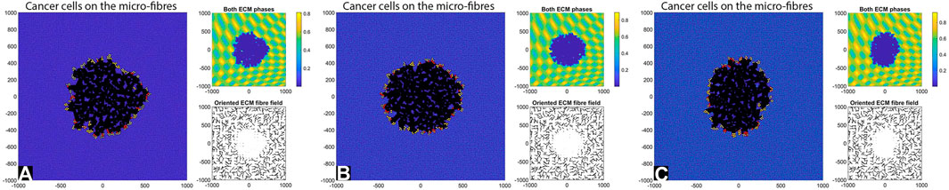
FIGURE 5. Simulation results at final time T = 28 days with random fibres, sensing radius $R=50\mu m$, repulsion $F^{rep}=0.45\times 10mg/\mu m\cdot {\min }^2$, cell-cell adhesion $F^{\text{adh}}=0.12\times 10mg/\mu m\cdot mi{n}^2$, cell-non-fibre ECM adhesion $S_{cl}=0$, cell-fibre ECM adhesion $S_{cF}=0$ and with (A) $10\%:90\%$, (B) $20\%:80\%$, (C) $30\%:70\%$ fibres and non-fibres ECM ratios. For illustrative purposes, all oriented ECM fibre fields are coarsened four-fold. Initial cell position was: (A–C) (0,0).

By comparing the numerical results in Figures 4, 5 we can conclude that in the absence of any cell-ECM adhesion, the tumour colonies have an almost circular shape, and they are stationary (i.e., they do not move through the domain). Moreover, the larger cell sensing radius does not seem to have a significant impact on tumour structure.

Simulations With Cell-ECM Adhesions in a Random Fibrous Environment

Next, we consider cell-ECM adhesion forces ($S_{cl}=0.01$, $S_{cF}=1.8$), and investigate again the effect of changes in fibre ECM density (i.e., 10–30–% fibres), for two different sensing radii: $R=30\mu m$ in Figure 6, and $R=50\mu m$ in Figure 7. Since now we consider cell-ECM interactions, in these two figures we also show model dynamics when the ECM environment is described by random fibres [sub-panels (A)-(C)] or by aligned fibres [sub-panels (A’)-(C’)].

FIGURE 6

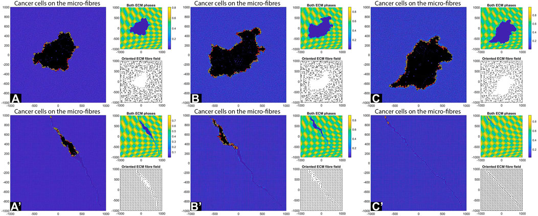
FIGURE 6. Simulation results with random and aligned fibres, sensing radius $R=30\mu m$, repulsion $F^{rep}=0.9\times 10mg/\mu m\cdot {\min }^2$, cell-cell adhesion $F^{\text{adh}}=0.12\times 10mg/\mu m\cdot mi{n}^2$, cell-non-fibre ECM adhesion $S_{cl}=0.01$, cell-fibre ECM adhesion $S_{cF}=1.8$ and with (A–A′) $10\text{\%}:90\text{\%}$, (B–B′) $20\%:80\%$, (C–C′) $30\%:70\%$ fibres and non-fibres ECM ratios. In (A–C) the fibre orientation field is set to be random and in (A′–C′) it is set to be aligned. Moreover the final simulation times are (A–C) T = 28 days, (A′) T = 14294 minutes, (B′) T = 10761 minutes and (C′) T = 4169 minutes. For illustrative purposes, all oriented ECM fibre fields are coarsened four-fold. Initial cell position was: (A–C) (0,0), (A′–,C′) (900, −900).

FIGURE 7

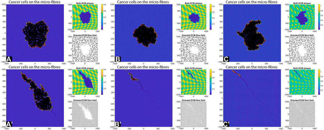
FIGURE 7. Simulation results with random and aligned fibres, sensing radius $R=50\mu m$, repulsion $F^{rep}=0.9\times 10mg/\mu m\cdot {\min }^2$, cell-cell adhesion $F^{adh}=0.12\times 10mg/\mu m\cdot {\min }^2$, cell-non-fibre ECM adhesion $S_{cl}=0.01$, cell-fibre ECM adhesion $S_{cF}=1.8$ and with (A−A′) $10\%:90\%$, (B−B′) $20\%:80\%$, (C−C′) $30\%:70\%$ fibres and non-fibres ECM ratios. In (A−C) the fibre orientation field is set to be random and in (A′–C′) it is set to be aligned. Moreover the final simulation times are (A–C) T = 28 days, (A′) T = 28470 minutes, (B′) T = 9260 minutes and (C′) T = 6351 minutes. For illustrative purposes, all oriented ECM fibre fields are coarsened four-fold. Initial cell position was: (A–C) (0,0), (A′–C′) (900, −900).

First, we see that cell-ECM interactions can lead to irregular-shaped tumour aggregations as well as elongated tumour aggregations. The random fibres are associated with stationary cell aggregations [sub-panels (A)-(C)], while the aligned fibres are associated with moving cell aggregations [sub-panels (A’)–(C’)].

The increase in sensing region (from $R=30$ in Figure 6 to $R=50$ in Figure 7) leads to an important difference. Even though we have now introduced the cell-ECM adhesion, in a lower fibre ECM density (10–20%) the tumour still kept its more round shape due to the increase of the sensing region. One possible explanation for this is that by increasing the sensing region in a random ECM environment, the different forces that emerge from the fibre orientations, cancel each other out and so the cancer cells are not subject to a strong leading force.

Finally, the increase in cell sensing radius to $R=50$ in an aligned fibrous environment, leads to a more compact tumour aggregation for the case of 10: 90% fibres: non-fibres ECM ratios. For higher ratios, the tumour is extremely elongated and the sensing radius has almost no impact.

Decreasing the Cell-Cell Adhesion Strength

Previous simulations were performed with a relatively high cell-cell adhesion strength ($F^{adh}=0.12$), which impacts the overall shape of tumour aggregations. Let us now decrease the cell-cell adhesion strength and consider $F^{adh}=0.04$ (while keeping all other parameters as before). In Figures 8, 9 we can see that a decrease in cell-cell adhesion causes more irregularly-shaped tumour aggregations. This is counterbalanced a bit by an increase in the sensing radius to $R=50$ which, as before, tends to favorise more round-shaped tumour aggregations.

FIGURE 8

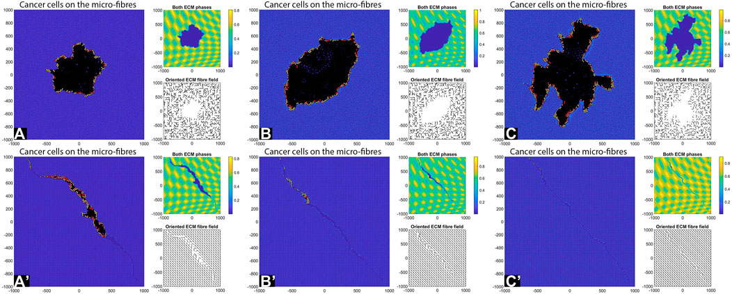
FIGURE 8. Simulation results with random and aligned fibres, sensing radius $R=30\mu m$, repulsion $F^{rep}=0.9\times 10mg/\mu m\cdot {\min }^2$, cell-cell adhesion $F^{\text{adh}}=0.04\times 10mg/\mu m\cdot mi{n}^2$, cell-non-fibre ECM adhesion $S_{cl}=0.01$, cell-fibre ECM adhesion $S_{cF}=1.8$ and with (A–A′) $10\%:90\%$, (B–B′) $20\%:80\%$, (C–C′) $30\%:70\%$ fibres and non-fibres ECM ratios. In (A–C) the fibre orientation field is set to be random and in (A′–C′) it is set to be aligned. Moreover the final simulation times are (A–C) T = 28 days, (A′) T = 11860 min, (B′) T = 6822 min and (C′) T = 3378 min. For illustrative purposes, all oriented ECM fibre fields are coarsened four-fold. Initial cell position was: (A–C) (0,0), (A′–C′) (900,−900).

FIGURE 9

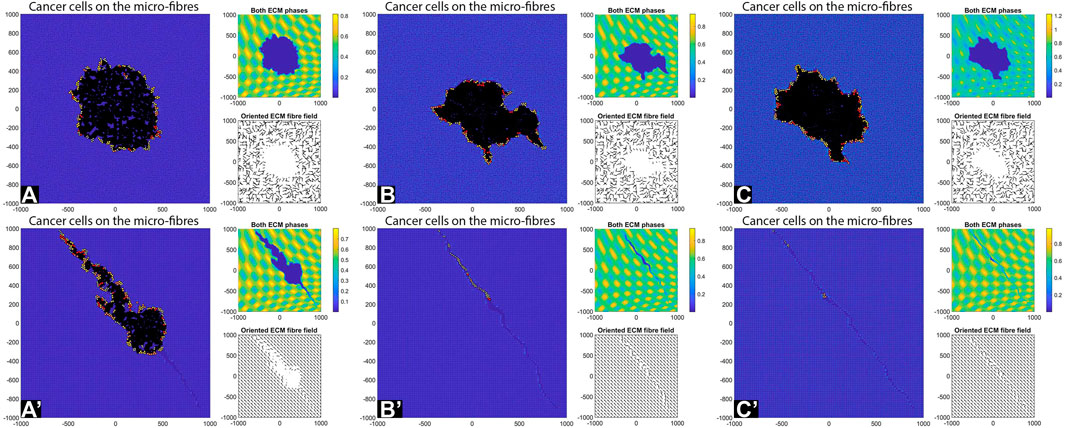
FIGURE 9. Simulation results with random and aligned fibres, sensing radius $R=50\mu m$, repulsion $F^{rep}=0.9\times 10mg/\mu m\cdot {\min }^2$, cell-cell adhesion $F^{adh}=0.04\times 10mg/\mu m\cdot {\min }^2$, cell-non-fibre ECM adhesion $S_{cl}=0.01$, cell-fibre ECM adhesion $S_{cF}=1.8$ and with (A–A′) $10\%:90\%$, (B–B′) $20\%:80\%$, (C–C′) $30\%:70\%$ fibres and non-fibres ECM ratios. In (A–C) the fibre orientation field is set to be random and in (A′–C′) it is set to be aligned. Moreover the final simulation times are (A–C) T = 28 days, (A′) T = 21400 min, (B′) T = 6551 min and (C′) T = 4305 minutes. For illustrative purposes, all oriented ECM fibre fields are coarsened four-fold. Initial cell position was: (A–C) (0,0), (A′–C′) (900,−900).

Decreasing the Cell-Fibre ECM Adhesion Strength

Since the previous simulations had low cell-cell adhesion but high cell-fibre ECM adhesion, next we investigate tumour invasion patterns when we lower the cell-fibre adhesion strength to $S_{cF}=1.2$ (while keeping $F^{adh}=0.04$). In Figures 10, 11 we see that lowering cell-fibre adhesion leads to a highly-irregular tumour shape, especially for the case of $30\%:70\%$ fibres to non-fibres ECM ratios.

FIGURE 10

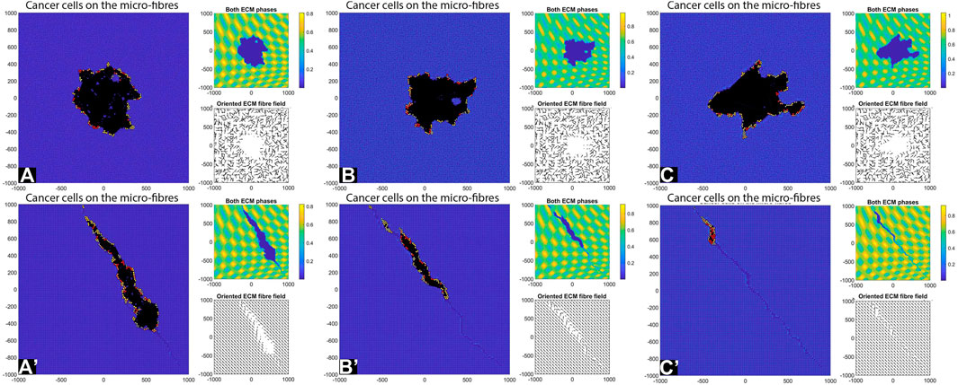
FIGURE 10. Simulation results with random and aligned fibres, sensing radius $R=30\mu m$, repulsion $F^{rep}=0.75\times 10mg/\mu m\cdot {\min }^2$, cell-cell adhesion $F^{\text{adh}}=0.04\times 10mg/\mu m\cdot mi{n}^2$, cell-non-fibre ECM adhesion $S_{cl}=0.01$, cell-fibre ECM adhesion $S_{cF}=1.2$ and with (A–A′) $10\%:90\%$, (B–B′) $20\%:80\%$, (C–C′) $30\%:70\%$ fibres and non-fibres ECM ratios. In (A–C) the fibre orientation field is set to be random and in (A′–C′) it is set to be aligned. Moreover the final simulation times are (A–C) T = 28 days, (A′) T = 20183 min, (B′) T = 12268 min and (C′) T = 7589 minutes. For illustrative purposes, all oriented ECM fibre fields are coarsened four-fold. Initial cell position was: (A–C) (0,0), (A′–C′) (900,−900).

FIGURE 11

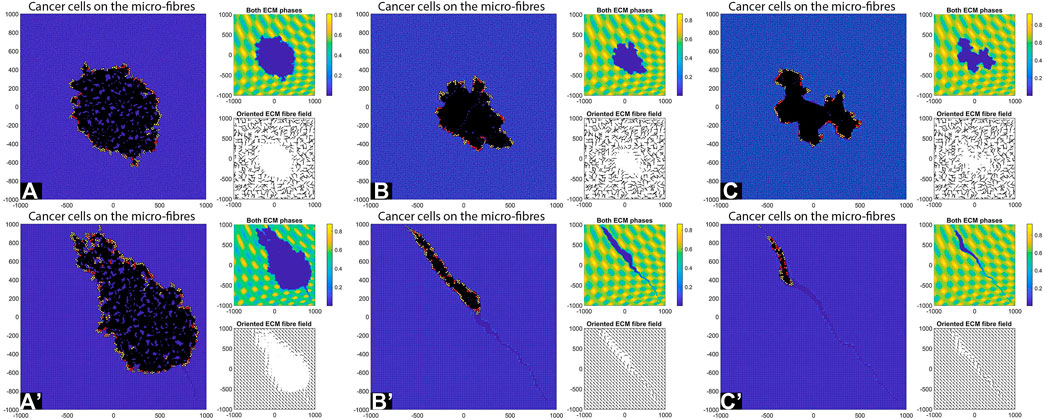
FIGURE 11. Simulation results with random and aligned fibres, sensing radius $R=50\mu m$, repulsion $F^{\text{rep}}=0.75\times 10mg/\mu m\cdot mi{n}^2$, cell-cell adhesion $F^{\text{adh}}=0.04\times 10mg/\mu m\cdot mi{n}^2$, cell-non-fibre ECM adhesion $S_{cl}=0.01$, cell-fibre ECM adhesion $S_{cF}=1.2$ and with (A–A′) $10\text{\%}:90\text{\%}$, (B–B′) $20\text{\%}:80\text{\%}$, (C–C′) $30\text{\%}:70\text{\%}$ fibres and non-fibres ECM ratios. In (A–C) the fibre orientation field is set to be random and in (A′–C′) it is set to be aligned. Moreover the final simulation times are (A–C) T = 28 days, (A′) T = 37517 min, (B′) T = 14220 min and (C′) T = 9982 min. For illustrative purposes, all oriented ECM fibre fields are coarsened four-fold. Initial cell position was: (A–C) (0,0), (A′–C′) (900,−900).

Consider now an even lower cell-ECM adhesion strength, $S_{cF}=0.3$, and at the same time a lower cell repulsion $F^{rep}=0.5$. In Figures 12, 13 we see that tumour aggregations have recovered their circular shape when the ECM fibres are distributed randomly, and have either circular or slightly elongated structures when the ECM fibres are aligned.

FIGURE 12

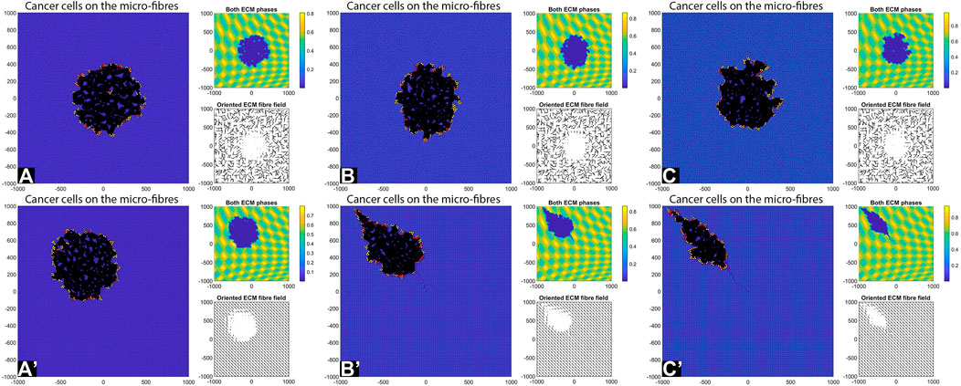
FIGURE 12. Simulation results with random and aligned fibres, sensing radius $R=30\mu m$, repulsion $F^{rep}=0.5\times 10mg/\mu m\cdot {\min }^2$, cell-cell adhesion $F^{\text{adh}}=0.12\times 10mg/\mu m\cdot mi{n}^2$, cell-non-fibre ECM adhesion $S_{cl}=0.01$, cell-fibre ECM adhesion $S_{cF}=0.3$ and with (A–A′) $10\text{\%}:90\text{\%}$, (B–B′) $20\text{\%}:80\text{\%}$, (C–C′) $30\text{\%}:70\text{\%}$ fibres and non-fibres ECM ratios. In (A–C) the fibre orientation field is set to be random and in (A′–C′) it is set to be aligned. Moreover the final simulation times are (A, A′, B, C) T = 28 days, (B′) T = 34707 min and (C′) T = 25801 min. For illustrative purposes, all oriented ECM fibre fields are coarsened four-fold. Initial cell position was: (A–C′) (0,0).

FIGURE 13

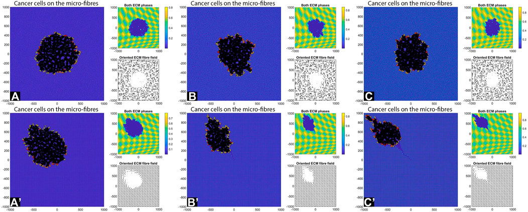
FIGURE 13. Simulation results with random and aligned fibres, sensing radius $R=50\mu m$, repulsion $F^{rep}=0.5\times 10mg/\mu m\cdot {\min }^2$, cell-cell adhesion $F^{\text{adh}}=0.12\times 10mg/\mu m\cdot mi{n}^2$, cell-non-fibre ECM adhesion $S_{cl}=0.01$, cell-fibre ECM adhesion $S_{cF}=0.3$ and with (A–A′) $10\%:90\%$, (B–B′) $20\%:80\%$, (C–C′) $30\%:70\%$ fibres and non-fibres ECM ratios. In (A,B–C) the fibre orientation field is set to be random and in (A′–C′) it is set to be aligned. Moreover the final simulation times are (A, A′, B, C) T = 28 days, (B′) T = 31873 min and (C′) T = 31506 minutes. For illustrative purposes, all oriented ECM fibre fields are coarsened four-fold. Initial cell position was: (A–C′) (0,0).

We emphasise that the simulations in sub-panels (B’)–(C’) in the above figures were ran for shorter times, since for longer times the cells leave the domain.

Different Tissues With Different Fibre Orientations

Finally, we investigate numerically what happens with tumour shape and its invasion pattern when the ECM domain is formed of patches of random and aligned fibres, corresponding to different types of tissues (see the discussion in the Introduction). For this we start with a cluster of cells (e.g., 19 cells, for illustration purposes) instead of just one cell. Moreover, we consider here again the parameter values used for the results in Figures 6C–C′, namely: $R=30\mu m$, $F^{\text{rep}}=0.9$, $F^{\text{adh}}=0.12$, $S_{cl}=0.01$, $S_{cF}=1.8$, and $30\%:70\%$ fibres and non-fibres ECM ratios. In Figure 14 we present six scenarios corresponding to different regions of random and aligned ECM fibres. In sub-panels (A)–(C) we plot the distribution of cancer cells and the ECM degradation pattern at a single time snapshot [i.e., (A) T = 5283 min, (B) T = 4601 min, (C) T = 9518 min]. In panels (D)–(F) we plot the distribution of cancer cells and the ECM degradation patterns at three different times (T = 9500 min, T = 15000 min, T = 20000 min), to illustrate the time-evolution of the system.

FIGURE 14

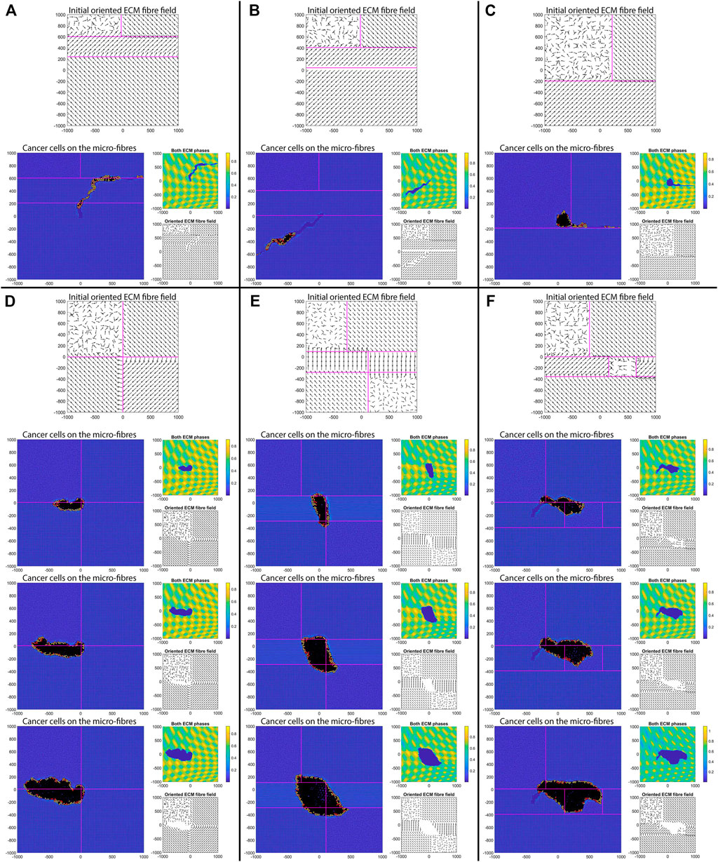
FIGURE 14. Simulation results with different aligned fibre structures, sensing radius $R=30\mu m$, repulsion $F^{rep}=0.9\times 10mg/\mu m\cdot {\min }^2$, cell-cell adhesion $F^{\text{adh}}=0.12\times 10mg/\mu m\cdot mi{n}^2$, cell-non-fibre ECM adhesion $S_{cl}=0.01$, cell-fibre ECM adhesion $S_{cF}=1.8$ and with $30\%:70\%$ fibres and non-fibres ECM ratios. In the first row of each panel (A–F), we present the four-fold coarsened initial oriented ECM fibre field and the purple lines represent the dividing lines between the regions with different tissue alignments. In panel (A) we plot a single result at time T = 5283 min, in (B) at time T = 4601 min and in (C) at time T = 9518. In panels (D–F) we plot the results at three different times to illustrate the evolution of the tumour, specifically, we use T = 9500, T = 15000, T = 20000 minutes, respectively. The oriented ECM fibres fields are coarsened four-fold for illustration purposes. Initial center of cell cluster position was: (A–E) (0,0), (F) (−400, −200).

The simulations in Figure 14 show that the initial position of the cluster of tumour cells, together with the ECM alignment in that region, influences the direction of migration of these cells. In sub-panels (A)–(B) the cells migrate in the direction of fibre alignment, while in sub-panel (C) the cells migrate along the boundary between two regions with opposite alignment. A similar migration pattern is observed in sub-panel (D). Finally, in sub-panels (E) and (F) we observe that when the original tumour cell cluster is positioned in an area surrounded by different ECM alignment, the tumour tends to stay in that area and to very slowly invade the neighbouring tissues (with different ECM orientations). All these different tumour invasive patterns are consistent with the experimental results in [10, 52], which showed that aligned collagen fibres perpendicular to tumour boundary are associated with tumour invasion along those fibres, and the experiments in [52] which showed that aligned collagen fibres parallel to tumour boundary impede invasion.

Summary and Discussion

The composition and structural characteristics of the extracellular matrix (ECM) are known to vary widely among different tissues [11], and this has a significant impact on the evolution of cancer. Since there is an increasing need for understanding the spatio-temporal changes in ECM and their roles in cancer progression, in this study we introduced a new multi-scale hybrid mathematical model for cell-cell and cell-ECM interactions, and used it to investigate numerically the impact of ECM fibre orientation and fibre density on cancer cell invasion patterns. To this end, we varied a number of parameters associated with the cell-cell interactions (e.g., cell sensing radius R, cell-cell adhesion stiffness $F^{adh}$, cell-cell repulsion stiffness $F^{rep}$), and parameters associated with cell-ECM interactions (i.e., cell-fibre adhesion coefficient $S_{cF}$, and cell-non-fibre adhesion coefficient $S_{cl}$), as well as we varied the random or aligned distribution of fibres. This enables us to explore their impact on the formation of cell aggregations and their collective dynamics.

Through numerical simulations, we tested a variety of scenarios: from the impact of smaller/larger cell sensing radius on tumour aggregations, to the impact of random vs. aligned fibres on the migration and invasion of cancer cells into nearby tissues, the role of different fibre orientation in the neighbourhood of initial tumour, and the roles of cell-cell and cell-ECM strengths on the shape of solid tumours. We summarise all these numerical results in Table 1 (for the case $R=30\mu m$) and Table 2 (for the case $R=50\mu m$). By comparing the $3^{rd}$ column (Description) with the 10th column (Fibre orientation) it is clear that a random ECM fibre distribution leads to stationary tumour aggregations, while an oriented fibre distribution leads to moving tumour aggregations. These numerical results are consistent with experimental results showing that oriented collagen fibres direct tumour invasion, with the alignment of collagen fibres coinciding with the cell invasive direction [10, 53]. Moreover, our numerical results in Figure 14 showed that collagen fibres that are relatively parallel to tumour boundary (and create a capsule-like orientation) can limit tumour invasion. These results are consistent with a recent note by Friedl [54], as well as the experiments in [52], about to the importance of ECM orientation relative to the tumour (see also Figure 1 in [54]).

TABLE 1

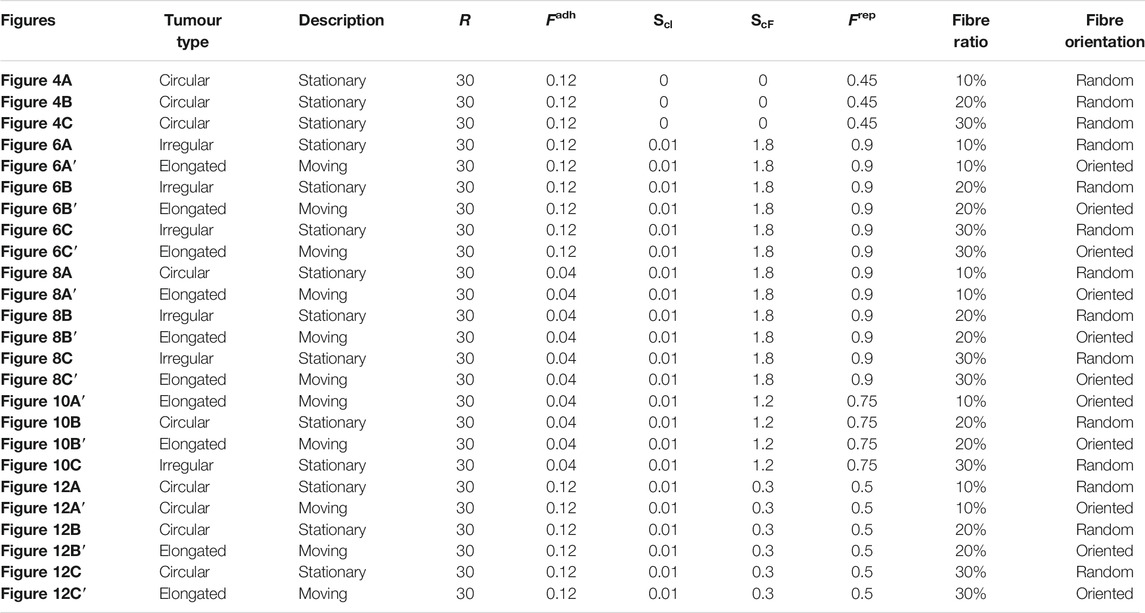
TABLE 1. Summary of numerical results obtained for a cell sensing radius of $R=30\mu m$.

TABLE 2

TABLE 2. Summary of numerical results obtained for a cell sensing radius of $R=50\mu m$.

The results in Figure 14 suggest that if we could know the orientation of collagen fibres surrounding the tumour (which may be spanning different tissues with different ECM structures) we could predict the fast or slow evolution of the solid tumour, as well as potential cell migration directions. Since collagen can be easily visualised in standard histopathology slides through second harmonic generation microscopy [10] or via multiphoton tomography [55], such predictions on the evolution of tumours might help treatment decisions, e.g., by deciding to resect more surrounding tissue if the imaging shows collagen fibres aligned perpendicular to tumour boundary in a certain area, or by deciding to preserve more surrounding tissue if the imaging shows collagen fibres parallel to tumour boundary. Intraoperative visualisation of tumour microenvironment, including collagen alignment in resected tissues [56], could be further combined with mathematical simulations in 2D (and even in 3D, although this is expected to carry a considerably higher computational cost) to improve such treatment decisions.

Finally, our numerical simulations suggest that the sensing radius R (determined by the length of membrane protrusions called pseudopodia [50, 51], as well as by the long-range sensing due to stress transmission via aligned ECM fibres [13]) impacts the shape of tumour colonies in an aligned fibrous ECM environment with relatively low ratios of fibres to non-fibres. More precisely, when the ECM ratio of fibres to non-fibres is 10%: 90%, larger R leads to more compact tumor cell colonies (compare with the cluster invasion pattern in [12]). For higher fibres: non-fibres ratios this sensing radius has almost no impact, the tumour being extremely elongated as the cells move quickly along the collagen fibres (compare with the strands and files patterns in [12]).

Overall, this study not only confirmed some of the previous experimental results on the importance of alignement of ECM collagen fibres on tumour invasion [10, 52], but also proposed new hypotheses on the biological mechanisms involved in the shape of the tumour colonies (e.g., the roles of sensing radius vs. fibres to non-fibres ratios; the roles of sensing radius vs. cell-cell and cell-ECM mechanical forces). Moreover, this multi-scale hybrid modelling, which incorporates ECM remodelling and fibre rearrangement in the direction of cell travelling (via cell flux $\mathrm{ℱ}\left(x,t\right)$), can be further applied to understand various other fibrotic diseases characterised by ECM remodelling [57].

Data Availability Statement

The original contributions presented in the study are included in the article/Supplementary Material, further inquiries can be directed to the corresponding author.

Author Contributions

All authors listed have made a substantial, direct, and intellectual contribution to the work and approved it for publication.

Funding

This work was supported by an EPSRC UK award, EPSRC DTA EP/R513192/1, and by the National Institutes of Health, National Cancer Institute Grant NIH/NCI U01-CA202229 (to KR).

Conflict of Interest

The authors declare that the research was conducted in the absence of any commercial or financial relationships that could be construed as a potential conflict of interest.

References

1. Walker, C, Mojares, E, and del Río Hernández, A. Role of Extracellular Matrix in Development and Cancer Progression. Int J Mol Sci (2018). 19:3028. doi:10.3390/ijms19103028

PubMed Abstract | CrossRef Full Text | Google Scholar

2. Xu, S, Xu, H, Wang, W, Li, S, Li, H, Li, T, et al. The Role of Collagen in Cancer: from Bench to Bedside. J Transl Med (2019). 17:309. doi:10.1186/s12967-019-2058-1

PubMed Abstract | CrossRef Full Text | Google Scholar

3. Padhi, A, and Nain, AS. ECM in Differentiation: A Review of Matrix Structure, Composition and Mechanical Properties. Ann Biomed Eng (2019). 48:1071–89. doi:10.1007/s10439-019-02337-7

PubMed Abstract | CrossRef Full Text | Google Scholar

4. Lin, J, Shi, Y, Men, Y, Wang, X, Ye, J, and Zhang, C. Mechanical Roles in Formation of Oriented Collagen Fibers. Tissue Eng B: Rev (2020). 26:116–28. doi:10.1089/ten.teb.2019.0243

PubMed Abstract | CrossRef Full Text | Google Scholar

5. Yasui, T, Tohno, Y, and Araki, T. Determination of Collagen Fiber Orientation in Human Tissue by Use of Polarisation Measurement of Molecular Second-Harmonic-Generation Light. Appl Opt (2004). 43:2861–7. doi:10.1364/ao.43.002861

PubMed Abstract | CrossRef Full Text | Google Scholar

6. Suda, K, Abe, K, and Kaneda, K. Changes in the Orientation of Collagen Fibers on the Superficial Layer of the Mouse Tibial Bone after Denervation. Scanning Electron Microscopic Observations. Arch Histology Cytol (1999). 62:231–5. doi:10.1679/aohc.62.231

PubMed Abstract | CrossRef Full Text | Google Scholar

7. Holmes, DF, Gilpin, CJ, Baldock, C, Ziese, U, Koster, AJ, and Kadler, KE. Corneal Collagen Fibril Structure in Three Dimensions: Structural Insights into Fibril Assembly, Mechanical Properties, and Tissue Organization. Proc Natl Acad Sci (2001). 98:7307–12. doi:10.1073/pnas.111150598

PubMed Abstract | CrossRef Full Text | Google Scholar

8. Weber, KT. Cardiac Interstitium in Health and Disease: the Fibrillar Collagen Network. J Am Coll Cardiol (1989). 13:1637–52. doi:10.1016/0735-1097(89)90360-4

PubMed Abstract | CrossRef Full Text | Google Scholar

9. Lin, J, Pan, S, Zheng, W, and Huang, Z. Polarization-resolved Second-Harmonic Generation Imaging for Liver Fibrosis Assessment without Labeling. Appl Phys Lett (2013). 103:173701. doi:10.1063/1.4826516

CrossRef Full Text | Google Scholar

10. Conklin, MW, Eickhoff, JC, Riching, KM, Pehlke, CA, Eliceiri, KW, Provenzano, PP, et al. Aligned Collagen Is a Prognostic Signature for Survival in Human Breast Carcinoma. Am J Pathol (2011). 178:1221–32. doi:10.1016/j.ajpath.2010.11.076

PubMed Abstract | CrossRef Full Text | Google Scholar

11. Malandrino, A, Mak, M, Kamm, RD, and Moeendarbary, E. Complex Mechanics of the Heterogeneous Extracellular Matrix in Cancer. Extreme Mech Lett (2018). 21:25–34. doi:10.1016/j.eml.2018.02.003

PubMed Abstract | CrossRef Full Text | Google Scholar

12. Friedl, P, and Alexander, S. Cancer Invasion and the Microenvironment: Plasticity and Reciprocity. Cell (2011). 147:992–1009. doi:10.1016/j.cell.2011.11.016

PubMed Abstract | CrossRef Full Text | Google Scholar

13. Ma, X, Schickel, ME, Stevenson, MD, Sarang-Sieminski, AL, Gooch, KJ, Ghadiali, SN, et al. Fibers in the Extracellular Matrix Enable Long-Range Stress Transmission between Cells. Biophysical J (2013). 104:1410–8. doi:10.1016/j.bpj.2013.02.017

CrossRef Full Text | Google Scholar

14. Schaller, G, and Meyer-Hermann, M. Continuum versus Discrete Model: a Comparison for Multicellular Tumour Spheroids. Phil Trans R Soc A (2006). 364:1443–64. doi:10.1098/rsta.2006.1780

PubMed Abstract | CrossRef Full Text | Google Scholar

15. Chamseddine, IM, and Rejniak, KA. Hybrid Modeling Frameworks of Tumor Development and Treatment. Wires Syst Biol Med (2020). 12:e1461. doi:10.1002/wsbm.1461

CrossRef Full Text | Google Scholar

16. Kim, M, Reed, D, and Rejniak, KA. The Formation of Tight Tumor Clusters Affects the Efficacy of Cell Cycle Inhibitors: A Hybrid Model Study. J Theor Biol (2014). 352:31–50. doi:10.1016/j.jtbi.2014.02.027

PubMed Abstract | CrossRef Full Text | Google Scholar

17. Karolak, A, Poonja, S, and Rejniak, KA. Morphophenotypic Classification of Tumor Organoids as an Indicator of Drug Exposure and Penetration Potential. Plos Comput Biol (2019). 15:e1007214. doi:10.1371/journal.pcbi.1007214

PubMed Abstract | CrossRef Full Text | Google Scholar

18. Berrouet, C, Dorilas, N, Rejniak, KA, and Tuncer, N. Comparison of Drug Inhibitory Effects (IC₅₀) in Monolayer and Spheroid Cultures. Bull Math Biol (2020). 82:68. doi:10.1007/s11538-020-00746-7

PubMed Abstract | CrossRef Full Text | Google Scholar

19. Shuttleworth, R, and Trucu, D. Multiscale Modelling of Fibres Dynamics and Cell Adhesion within Moving Boundary Cancer Invasion. Bull Math Biol (2019). 81:2176–219. doi:10.1007/s11538-019-00598-w

PubMed Abstract | CrossRef Full Text | Google Scholar

20. Shuttleworth, R, and Trucu, D. Cell-scale Degradation of Peritumoural Extracellular Matrix Fibre Network and its Role within Tissue-Scale Cancer Invasion. Bull Math Biol (2020). 82:65. doi:10.1007/s11538-020-00732-z

PubMed Abstract | CrossRef Full Text | Google Scholar

21. Shuttleworth, R, and Trucu, D. Multiscale Dynamics of a Heterotypic Cancer Cell Population within a Fibrous Extracellular Matrix. J Theor Biol (2020). 486:110040. doi:10.1016/j.jtbi.2019.110040

PubMed Abstract | CrossRef Full Text | Google Scholar

22. Suveges, S, Eftimie, R, and Trucu, D. Directionality of Macrophages Movement in Tumour Invasion: A Multiscale Moving-Boundary Approach. Bull Math Biol (2020). 82. doi:10.1007/s11538-020-00819-7

PubMed Abstract | CrossRef Full Text | Google Scholar

23. Suveges, S, Eftimie, R, and Trucu, D. Re-polarisation of Macrophages within a Multi-Scale Moving Boundary Tumour Invasion Model. arXiv:2103.03384 (2021). 1–50.

Google Scholar

24. Alberts, B, Johnson, A, Lewis, J, Raff, M, Roberts, K, and Walter, P. Molecular Biology of the Cell. New York: Garland Science (2002).

25. Tyson, JJ, and Novak, B. Temporal Organization of the Cell Cycle. Curr Biol (2008). 18:R759–R768. doi:10.1016/j.cub.2008.07.001

PubMed Abstract | CrossRef Full Text | Google Scholar

26. Pérez-Velázquez, J, and Rejniak, KA. Drug-Induced Resistance in Micrometastases: Analysis of Spatio-Temporal Cell Lineages. Front Physiol (2020). 11:319. doi:10.3389/fphys.2020.00319

PubMed Abstract | CrossRef Full Text | Google Scholar

27. Cooper, G. The Cell : A Molecular Approach. Washington, D.C. Sunderland, Mass: ASM Press Sinauer Associates (2000).

28. Huda, S, Weigelin, B, Wolf, K, Tretiakov, KV, Polev, K, Wilk, G, et al. Lévy-like Movement Patterns of Metastatic Cancer Cells Revealed in Microfabricated Systems and Implicated In Vivo. Nat Commun (2018). 9:4539. doi:10.1038/s41467-018-06563-w

PubMed Abstract | CrossRef Full Text | Google Scholar

29. Petrie, RJ, Doyle, AD, and Yamada, KM. Random versus Directionally Persistent Cell Migration. Nat Rev Mol Cel Biol (2009). 10:538–49. doi:10.1038/nrm2729

CrossRef Full Text | Google Scholar

30. Weiger, MC, Vedham, V, Stuelten, CH, Shou, K, Herrera, M, Sato, M, et al. Real-time Motion Analysis Reveals Cell Directionality as an Indicator of Breast Cancer Progression. PLOS ONE (2013). 8:e58859–12. doi:10.1371/journal.pone.0058859

PubMed Abstract | CrossRef Full Text | Google Scholar

31. Wu, P-H, Giri, A, Sun, SX, and Wirtz, D. Three-dimensional Cell Migration Does Not Follow a Random Walk. Proc Natl Acad Sci (2014). 111:3949–54. doi:10.1073/pnas.1318967111

PubMed Abstract | CrossRef Full Text | Google Scholar

32. Ghosh, S, Salot, S, Sengupta, S, Navalkar, A, Ghosh, D, Jacob, R, et al. p53 Amyloid Formation Leading to its Loss of Function: Implications in Cancer Pathogenesis. Cell Death Differ (2017). 24:1784–98. doi:10.1038/cdd.2017.105

PubMed Abstract | CrossRef Full Text | Google Scholar

33. Gras, SL. Surface- and Solution-Based Assembly of Amyloid Fibrils for Biomedical and Nanotechnology Applications. In: RJ Koopmans, editor. Engineering Aspects of Self-Organizing Materials. Advances in Chemical Engineering, 35. Academic Press (2009). p. 161–209. doi:10.1016/S0065-2377(08)00206-8

CrossRef Full Text | Google Scholar

34. Gras, SL, Tickler, AK, Squires, AM, Devlin, GL, Horton, MA, Dobson, CM, et al. Functionalised Amyloid Fibrils for Roles in Cell Adhesion. Biomaterials (2008). 29:1553–62. doi:10.1016/j.biomaterials.2007.11.028

PubMed Abstract | CrossRef Full Text | Google Scholar

35. Jacob, RS, George, E, Singh, PK, Salot, S, Anoop, A, Jha, NN, et al. Cell Adhesion on Amyloid Fibrils Lacking Integrin Recognition Motif. J Biol Chem (2016). 291:5278–98. doi:10.1074/jbc.m115.678177

PubMed Abstract | CrossRef Full Text | Google Scholar

36. Wolf, K, Alexander, S, Schacht, V, Coussens, LM, von Andrian, UH, van Rheenen, J, et al. Collagen-based Cell Migration Models In Vitro and In Vivo. Semin Cel Develop Biol (2009). 20:931–41. doi:10.1016/j.semcdb.2009.08.005

CrossRef Full Text | Google Scholar

37. Wolf, K, and Friedl, P. Extracellular Matrix Determinants of Proteolytic and Non-proteolytic Cell Migration. Trends Cel Biol (2011). 21:736–44. doi:10.1016/j.tcb.2011.09.006

CrossRef Full Text | Google Scholar

38. Armstrong, NJ, Painter, KJ, and Sherratt, JA. A Continuum Approach to Modelling Cell-Cell Adhesion. J Theor Biol (2006). 243:98–113. doi:10.1016/j.jtbi.2006.05.030

PubMed Abstract | CrossRef Full Text | Google Scholar

39. Gerisch, A, and Chaplain, MAJ. Mathematical Modelling of Cancer Cell Invasion of Tissue: Local and Non-local Models and the Effect of Adhesion. J Theor Biol (2008). 250:684–704. doi:10.1016/j.jtbi.2007.10.026

PubMed Abstract | CrossRef Full Text | Google Scholar

40. Domschke, P, Trucu, D, Gerisch, A, and A. J. Chaplain, M. Mathematical Modelling of Cancer Invasion: Implications of Cell Adhesion Variability for Tumour Infiltrative Growth Patterns. J Theor Biol (2014). 361:41–60. doi:10.1016/j.jtbi.2014.07.010

PubMed Abstract | CrossRef Full Text | Google Scholar

41. Domschke, P, Trucu, D, Gerisch, A, and Chaplain, MAJ (2017). Structured Models of Cell Migration Incorporating Molecular Binding Processes. J. Math. Biol. 75, 1517–1561. doi:10.1007/s00285-017-1120-y

Google Scholar

42. Peng, L, Trucu, D, Lin, P, Thompson, A, and Chaplain, MAJ. A Multiscale Mathematical Model of Tumour Invasive Growth. Bull Math Biol (2017). 79:389–429. doi:10.1007/s11538-016-0237-2

PubMed Abstract | CrossRef Full Text | Google Scholar

43. Nagase, H, Visse, R, and Murphy, G. Structure and Function of Matrix Metalloproteinases and TIMPs. Cardiovasc Res (2006). 69:562–73. doi:10.1016/j.cardiores.2005.12.002

PubMed Abstract | CrossRef Full Text | Google Scholar

44. Visse, R, and Nagase, H. Matrix Metalloproteinases and Tissue Inhibitors of Metalloproteinases. Circ Res (2003). 92:827–39. doi:10.1161/01.RES.0000070112.80711.3D

PubMed Abstract | CrossRef Full Text | Google Scholar

45. Hanahan, D, and Weinberg, RA. Hallmarks of Cancer: The Next Generation. Cell (2011). 144:646–74. doi:10.1016/j.cell.2011.02.013

PubMed Abstract | CrossRef Full Text | Google Scholar

46. Weinberg, RA. The Biology of Cancer. New York: Garland Science (2006).

47. Stix, B, Kähne, T, Sletten, K, Raynes, J, Roessner, A, and Röcken, C. Proteolysis of AA Amyloid Fibril Proteins by Matrix Metalloproteinases-1, -2, and -3. Am J Pathol (2001). 159:561–70. doi:10.1016/s0002-9440(10)61727-0

PubMed Abstract | CrossRef Full Text | Google Scholar

48. Liao, M-C, and Van Nostrand, WE. Degradation of Soluble and Fibrillar Amyloid β-Protein by Matrix Metalloproteinase (MT1-MMP) In Vitro. Biochemistry (2010). 49:1127–36. doi:10.1021/bi901994d

PubMed Abstract | CrossRef Full Text | Google Scholar

49. Yosida, K Functional Analysis. 6th ed. Springer-Verlag (1980).

50. Murphy, DA, and Courtneidge, SA. The 'ins' and 'outs' of Podosomes and Invadopodia: Characteristics, Formation and Function. Nat Rev Mol Cel Biol. (2012). 12:413–26. doi:10.1038/nrm3141

CrossRef Full Text | Google Scholar

51. Klemke, RL. Trespassing Cancer Cells: 'fingerprinting' Invasive Protrusions Reveals Metastatic Culprits. Curr Opin Cel Biol (2012). 24:662–9. doi:10.1016/j.ceb.2012.08.005

CrossRef Full Text | Google Scholar

52. Provenzano, PP, Inman, DR, Eliceiri, KW, Trier, SM, and Keely, PJ. Contact Guidance Mediated Three-Dimensional Cell Migration Is Regulated by Rho/ROCK-dependent Matrix Reorganization. Biophysical J (2008). 95:5374–84. doi:10.1529/biophysj.108.133116

CrossRef Full Text | Google Scholar

53. Han, W, Chen, S, Yuan, W, Fan, Q, Tian, J, Wang, X, et al. Oriented Collagen Fibers Direct Tumor Cell Intravasation. Proc Natl Acad Sci USA (2016). 113:11208–13. doi:10.1073/pnas.1610347113

PubMed Abstract | CrossRef Full Text | Google Scholar

54. Friedl, P. Rethinking Research into Metastasis. eLIFE (2019). 8:e53511. doi:10.7554/eLife.53511

PubMed Abstract | CrossRef Full Text | Google Scholar

55. Uchugonova, A, Zhao, M, Weinigel, M, Zhang, Y, Bouvet, M, Hoffman, RM, et al. Multiphoton Tomography Visualizes Collagen Fibers in the Tumor Microenvironment that Maintain Cancer-Cell anchorage and Shape. J Cel Biochem. (2013). 114:99–102. doi:10.1002/jcb.24305

CrossRef Full Text | Google Scholar

56. Sun, Y, You, S, Tu, H, Spillman, DR, Chaney, EJ, Marjanovic, M, et al. Intraoperative Visualization of the Tumor Microenvironment and Quantification of Extracellular Vesicles by Label-free Nonlinear Imaging. Sci Adv (2018). 4:eaau5603. doi:10.1126/sciadv.aau5603

PubMed Abstract | CrossRef Full Text | Google Scholar

57. Cox, TR, and Erler, JT. Remodeling and Homeostasis of the Extracellular Matrix: Implications for Fibrotic Diseases and Cancer. Dis Models Mech (2011). 4:165–78. doi:10.1242/dmm.004077

PubMed Abstract | CrossRef Full Text | Google Scholar

58. Shashni, B, Ariyasu, S, Takeda, R, Suzuki, T, Shiina, S, Akimoto, K, et al. Size-based Differentiation of Cancer and normal Cells by a Particle Size Analyzer Assisted by a Cell-Recognition Pc Software. Biol Pharm Bull (2018). 41:487–503. doi:10.1248/bpb.b17-00776

PubMed Abstract | CrossRef Full Text | Google Scholar

59.NCI. NCI-60 Human Tumor Cell Lines Screen [internet]. on line (2015). Available from: https://dtp.cancer.gov/discovery˙_development/̵nci- ̵60/.

Google Scholar

60. Baumgartner, W, and Drenckhahn, D. Transmembrane Cooperative Linkage in Cellular Adhesion. Eur J Cel Biol (2002). 81:161–8. doi:10.1078/0171-9335-00233

CrossRef Full Text | Google Scholar

61. Rejniak, KA, and Dillon, RH. A Single Cell-Based Model of the Ductal Tumour Microarchitecture. Comput Math Methods Med (2007). 8:51–69. doi:10.1080/17486700701303143

CrossRef Full Text | Google Scholar

62. Shimolina, LE, Izquierdo, MA, López-Duarte, I, Bull, JA, Shirmanova, MV, Klapshina, LG, et al. Imaging Tumor Microscopic Viscosity In Vivo Using Molecular Rotors. Sci Rep (2017). 7:41097. doi:10.1038/srep41097

PubMed Abstract | CrossRef Full Text | Google Scholar

Appendix A: parameter set

In Table 3 we summarise the parameter values (and parameter ranges) used throughout the numerical simulations performed in this study.

TABLE 3

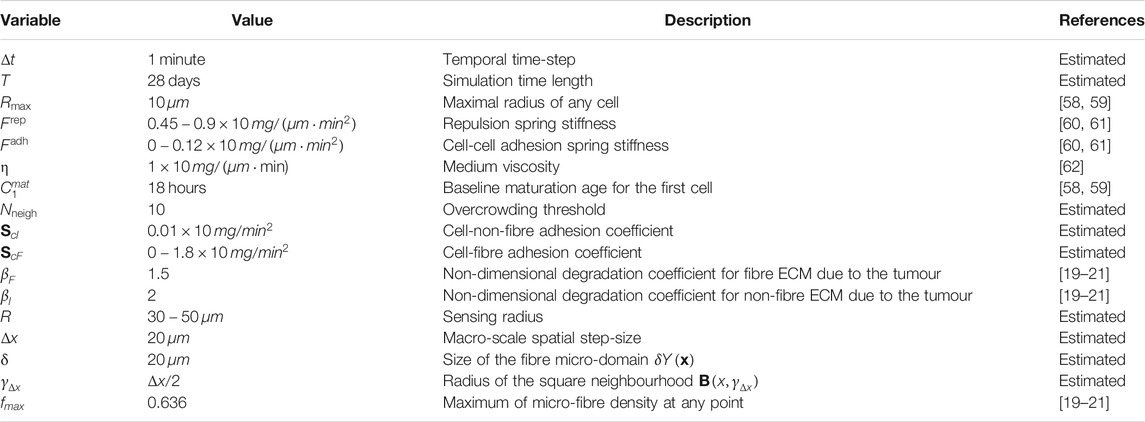
TABLE 3. Parameter set used for the numerical simulations presented in this study.

Appendix B: description of the connection between the individual-cells dynamics and continuum ecm dynamics

FIGURE 15

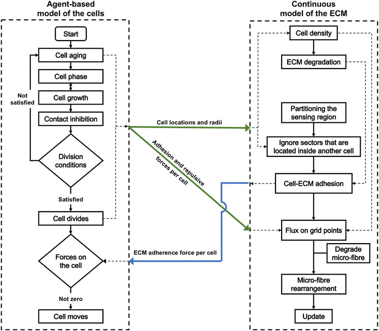
FIGURE 15. Diagrammatic description of the agent-based modelling of cells, the continuous modelling of the ECM and the connection of the two models at the specific stages of the numerical simulations.