Data-Space Inversion With a Recurrent Autoencoder for Naturally Fractured Systems

Introduction

Traditional model-based history matching entails the calibration of model parameters such that flow predictions match observed data, to within some tolerance. History matching, also referred to as data assimilation, represents an essential component of the overall reservoir management workflow, because without this calibration, predicted reservoir performance can be highly uncertain. Although model-based history matching approaches are well developed and widely applied, there are still some outstanding issues surrounding their characteristics and use. These include high computational demands, challenges associated with providing history matched (posterior) models that are fully consistent geologically with prior models, and lack of formal guarantees regarding posterior sampling.

Complementary approaches, referred to as data-space inversion procedures, have been developed in recent years. These methods do not provide posterior models but rather posterior predictions for key time-series of interest, such as well or field injection and production rates. Although their inability to generate posterior models represents a limitation in some application areas, DSI procedures have advantages over model-based methods in other settings. These include the ability to consider prior realizations from a range of different scenarios, decreased computational demands (in many cases), and flexibility in terms of data error and data weighting specifications. Data-space methods are commonly applied in conjunction with a data parameterization procedure. This allows data from prior realizations to be represented concisely and, ideally, assures that posterior data predictions (well-rate time series) display the correct physical character.

In recent work, we introduced a new data parameterization procedure and incorporated it into the DSI framework. This approach entails the use of a recurrent autoencoder in combination with a long short-term memory (LSTM) recurrent neural network. This treatment was shown to outperform existing approaches, including the use of principal component analysis with histogram transformation, and the direct use of time-series data without parameterization, for a set of idealized test cases. In this paper, we will explore the properties and behavior of this RAE-based parameterization for a complicated case based on an actual naturally fractured reservoir. We will, in particular, assess the ability of the new parameterization method to capture key correlations in the time-series production data. Accurately capturing such correlations is important for computing so-called derived quantities (i.e. quantities such as water cut that are constructed by combining data from one or more time series treated directly in DSI), and for quantifying uncertainty reduction when observations involve data of different types.

The basic DSI method applied here was originally developed by [1, 2]. DSI is formulated within a Bayesian framework, and different posterior sampling methods have been applied. In the original implementation [1–3], the randomized maximum likelihood method was used. Recent work by [4] demonstrated the advantages of ensemble smoother with multiple data assimilation (ESMDA) for posterior sampling. ESMDA was also found to perform well with our deep-learning-based DSI method [5].

A number of other methods that share some similarities with DSI have also been proposed. These include the prediction focused method originally developed by [6]. This approach entails the construction of a statistical relationship between observed data and the prediction objective in the parameterized latent space. Multivariate kernel density estimation [6], canonical correlation analysis [7–9], and artificial neural network with support vector regression [10] have been applied to build the relationship between observations and predictions in the low-dimensional space. When the latent space is not of very low dimension, however, these approaches may have difficulty capturing nonlinear data. The ensemble variance analysis (EVA) method developed by [11] represents another type of data-space method. This approach entails the construction of the cumulative distribution function for posterior results under a multi-Gaussian assumption. In [12], a nonlinear generalization of EVA was developed by applying nonlinear simulation regression with localization. EVA-based procedures, however, treat the various quantities of interest (QoI) individually, and thus do not fully capture the correlations between different QoI. In addition, they are not designed to provide time-series forecasts.

Data-space (and related) methods often apply some type of parameterization to provide a low-dimensional representation of the time-series data. Such a parameterization should, ideally, capture the complex physical behavior of, and correlations between, the various data streams. In [9, 10, 13], PCA was applied directly for dimension reduction and parameterization. PCA has also been combined with specialized mappings for time-series data with particular (problem-specific) characteristics [1]. This treatment was later generalized to a PCA procedure combined with histogram transformation, which was applied to noisy data resulting from multiple operational stages [2]. Nonlinear PCA [6] and functional data analysis methods [7, 8] have also been used to parameterize data from tracer flow and oil reservoir production problems. Recently, deep-learning based methods for time-series data, including auto-regressive [14] and recurrent neural network [15] treatments, were developed for reservoir forecasting. As noted earlier, our previous work entails the use of an LSTM-based RAE [5], which was shown to capture important correlations in time-series data.

A key goal of this work is to assess the performance of our new DSI treatments, previously demonstrated only for idealized cases, in a complicated real-field setting. The models considered here derive from an actual naturally fractured reservoir, though the operational specifications used in our examples represent one out of several possible scenarios. The field has over 10 years of primary production history, and a multiyear waterflood pilot involving two injectors with tracers is currently being planned to evaluate water injection as a potential full-field improved oil recovery (IOR) strategy. In this study, a large set of prior models (1850) is generated and simulated using an efficient workflow [16]. These models are based on nine discrete fracture network realizations and a range of matrix and fracture parameters (e.g. permeability, porosity, and rock compressibility). As a result of the multiple development stages considered, complex flow physics, and field-management logic (necessary for water and gas processing), the time-series data are quite complicated. Thus, this case represents a challenging test for the RAE-based parameterization. In this study, we are particularly interested in assessing the ability of the new parameterization to capture correlations in the waterflood pilot and full-field water injection forecasts, since pilot surveillance data will be used as indicators for future field performance [17]. It is important to note, however, that we do not use actual production data in our assessments here, but rather synthetic data. These data are derived from simulations of randomly selected realizations not used in the construction of the parameterizations. This approach enables us to avoid data-confidentiality issues and, importantly, allows us to assess DSI performance for multiple “true” models.

This paper proceeds as follows. In Section 2, we provide a concise review of the two data parameterization methods considered in this study and the overall DSI procedure. In Section 3, we describe the field and the models, and present results for the reconstruction of new (prior) data realizations not used in training. Correlations between data of different types will be considered. Posterior DSI predictions for primary and secondary quantities are presented in Section 4. Conclusion and suggestions for future work are provided in Section 5.

Data Parameterization and Data-Space Inversion

In this section, we first provide a review of the two data parameterization methods considered in this work–principal component analysis with histogram transformation (HT) [2], and the recurrent autoencoder procedure [5]. The use of these parameterizations in the DSI framework is then discussed.

Parameterization of Time-Series Data

In DSI, we use prior realizations of time-series data in combination with observed data to construct posterior data realizations. The generation of the prior data vectors, which is the time-consuming step in DSI, is accomplished by simulating a relatively large number (typically $\sim O\left(1000\right)$) of prior geological models. As noted earlier, in DSI, posterior models are not constructed–only posterior data realizations.

The generation of the prior ensemble of data vectors ${\mathbf{d}}_i$, $i=\mathrm{1,2},\dots ,N_{\text{r}}$, can be expressed as

${\mathbf{d}}_i=\mathbf{g}\left({\mathbf{m}}_i\right),(1)$

where $\text{g}$ represents the forward simulation process, $\text{m}$ denotes the geomodel, and $N_{\text{r}}$ is the number of prior models (and thus data vectors) considered. The data variables $\mathbf{d}\in {\mathrm{ℝ}}^{N_{\text{f}}\times 1}$ include a concatenation of the time-series flow rates for key QoI. These can include injection and production rates at wells, or time series at a sector or field level. In this work, we consider $N_{\text{QoI}}$ quantities of interest and $N_{\text{t}}$ simulation time steps. We thus have $N_{\text{f}}=N_{\text{QoI}}\times N_{\text{t}}$ as the dimension of each $\text{d}$ vector.

The data vectors typically follow high-dimensional non-Gaussian distributions as a result of the strongly nonlinear forward simulation process and the heterogeneous property fields that characterize the geomodels. Data parameterization enables us to use low-dimensional latent variables, $\mathit{\xi }\in {\mathrm{ℝ}}^{N_{\text{l}}\times 1}$, where $N_{\text{l}}$ denotes the number of latent variables, to represent $\mathbf{d}$. The parameterized data $\tilde{\text{d}}$ are then represented as $\tilde{\mathbf{d}}=\mathbf{f}\left(\mathit{\xi }\right)$, where $\mathbf{f}$ indicates the parameterization function. An ideal $\mathbf{f}$ should preserve the physical character and correlations in the high-dimensional time-series data, and it should accomplish this with $N_{\text{l}}\ll N_{\text{f}}$. It is advantageous to have $N_{\text{l}}\ll N_{\text{f}}$ as this reduces complications associated with high-dimensional inversion. Potential problems that may be avoided include ensemble collapse with ensemble-based methods (as are applied in this work) and issues related to high-dimensional minimization with optimization-based methods.

PCA With Histogram Transformation

Sun et al. [2] applied PCA with histogram transformation for the parameterization of noisy data. This approach is straightforward to use and it preserves the marginal distributions of the individual data variables, but it does not in general capture the correlations between different data variables (including correlations in time for a single QoI). The basic approach is as follows. The PCA basis matrix is constructed by performing singular value decomposition (SVD) of the data matrix $D\in {\mathrm{ℝ}}^{N_{\text{f}}\times N_{\text{r}}}$ containing centered prior realizations of d. Specifically,

$D=\frac{1}{\sqrt{N_{\text{r}}-1}}\left[{\mathbf{d}}_1-{\overline{\mathbf{d}}}_{\text{prior}}{\mathbf{d}}_2-{\overline{\mathbf{d}}}_{\text{prior}}{\text{…}\mathbf{d}}_{N_{\text{r}}}-{\overline{\mathbf{d}}}_{\text{prior}}\right]\text{,}(2)$

where ${\overline{\mathbf{d}}}_{\text{prior}}=\frac{1}{N_{\text{r}}}{\displaystyle {\sum }_{i=1}^{N_{\text{r}}}{\mathbf{d}}_i}$ is the mean of the prior data realizations. The SVD of matrix D provides the PCA basis matrix $\text{Φ}\in {\mathrm{ℝ}}^{N_{\text{f}}\times N_{\text{l}}}$. We apply an energy criterion to determine the latent space dimension $N_{\text{l}}$. See [2, 5] for full details.

With the PCA mapping, the latent-space prior vectors ${\mathit{\xi }}_i^{\text{PCA}}$, $i=\mathrm{1,2},\dots ,N_{\text{r}}$, are normally distributed [2]. The corresponding prior data vectors ${\mathbf{d}}_i^{\text{PCA}}$, $i=\mathrm{1,2},\dots ,N_{\text{r}}$, generated through application of ${\mathbf{d}}_i^{\text{PCA}}=\Phi {\mathit{\xi }}_i^{\text{PCA}}+{\overline{\mathbf{d}}}_{\text{prior}}$, are thus multi-Gaussian. Because the actual high-dimensional prior data variables are non-Gaussian, the PCA transformation may generate parameterized data realizations with nonphysical behavior. To partially mitigate such issues, histogram transformation is applied in a post-processing step. This maps the (Gaussian) PCA realizations ${\mathbf{d}}^{\text{PCA}}$ to match the prior marginal distributions associated with each component of the data realizations d. Specifically, let $f_T\left(\mathbf{d}\right)$ and $f_I\left({\mathbf{d}}^{\text{PCA}}\right)$ denote the cumulative distribution function (CDF) of the prior distribution of d (which is the target distribution) and the distribution of ${\mathbf{d}}^{\text{PCA}}$ (initial distribution), respectively. The parameterized data vector $\tilde{\mathbf{d}}$ is then generated through application of

$\tilde{\mathbf{d}}=h_T\left({\mathbf{d}}^{\text{PCA}}\right)=f_T^{-1}\left(f_I\left({\mathbf{d}}^{\text{PCA}}\right)\right),(3)$

where $h_T$ denotes the histogram transformation function.

As noted earlier, because histogram transformation for each component of ${\mathbf{d}}^{\text{PCA}}$ is applied independently, the joint distribution of the high-dimensional data will not be fully captured. The RAE-based parameterization, which we now describe, was developed in an attempt to maintain the complex correlations that characterize the prior (and thus posterior) data vectors.

RAE Procedure

The RAE-based time-series parameterization introduced by [5] involves an autoencoder and a long short-term memory (LSTM) network. The basic RAE architecture is shown in Figure 1. The encoder portion of the RAE maps the time-series data d to the low-dimensional latent variables ${\mathit{\xi }}^{\text{RAE}}$, while the decoder maps the low-dimensional representation back to high-dimensional (physical) space. LSTM networks are applied in both the encoder and decoder to capture and reconstruct the time-series data.

FIGURE 1

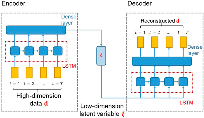
FIGURE 1. Schematic of RAE architecture (figure modified from [5]).

LSTM architectures, introduced by [18], are recurrent neural networks designed to capture both long-term and short-term information in time-series data. The LSTM unit for each time step t is composed of a neural network cell to store the temporal dynamics and three gates to regulate the input and output information. Let ${\mathbf{c}}_t\in {\mathrm{ℝ}}^{N_{\text{h}}\times 1}$ denote the cell state, where $N_{\text{h}}$ is the length of the cell state. For each LSTM unit at time step t, the input vector ${\mathbf{x}}_t\in {\mathrm{ℝ}}^{N_{\text{d}}\times 1}$ and the previous cell output (hidden) state ${\mathbf{h}}_{t-1}\in {\mathrm{ℝ}}^{N_{\text{h}}\times 1}$ are received and controlled by the forget gate ${\mathbf{f}}_t\in {\mathrm{ℝ}}^{N_{\text{h}}\times 1}$, the input gate ${\mathbf{i}}_t\in {\mathrm{ℝ}}^{N_{\text{h}}\times 1}$ and the output gate ${\mathbf{o}}_t\in {\mathrm{ℝ}}^{N_{\text{h}}\times 1}$. The gate operations are expressed as

$\begin{array}{l}{\mathbf{f}}_t=\sigma \left(W_f\left[{\mathbf{h}}_{t-1},{\mathbf{x}}_t\right]+{\mathbf{b}}_f\right),\\ {\mathbf{i}}_t=\sigma \left(W_i\left[{\mathbf{h}}_{t-1},{\mathbf{x}}_t\right]+{\mathbf{b}}_i\right),\\ {\mathbf{o}}_t=\sigma \left(W_o\left[{\mathbf{h}}_{t-1},{\mathbf{x}}_t\right]+{\mathbf{b}}_o\right),\end{array}(4)$

where $W\in {\mathrm{ℝ}}^{N_{\text{h}}\times \left(N_{\text{h}}+N_{\text{d}}\right)}$ denotes the weight matrix, $\mathbf{b}\in {\mathrm{ℝ}}^{N_{\text{h}}\times 1}$ is the bias term, and $\sigma (\cdot )$ is the (nonlinear) sigmoid function.

The candidate new cell state ${\tilde{\mathbf{c}}}_t$ is given by

${\tilde{\mathbf{c}}}_t=\text{tanh}\left(W_x\left[{\mathbf{h}}_{t-1},{\mathbf{x}}_t\right]+{\mathbf{b}}_c\right).(5)$

The cell state ${\mathbf{c}}_t$ at time step t involves the forget gate ${\mathbf{f}}_t$ applied to the previous cell state ${\mathbf{c}}_{t-1}$ and the input gate ${\mathbf{i}}_t$ applied to the candidate state ${\tilde{\mathbf{c}}}_t$, i.e.,

${\mathbf{c}}_t={\mathbf{f}}_t\circ {\mathbf{c}}_{t-1}+{\mathbf{i}}_t\circ {\tilde{\mathbf{c}}}_t,(6)$

where $\circ$ denotes the Hadamard product. The output gate ${\mathbf{o}}_t$ is then applied to provide the output state ${\mathbf{h}}_t$ via

${\mathbf{h}}_t={\mathbf{o}}_t\circ \text{tanh}\left({\mathbf{c}}_t\right).(7)$

The LSTM network is combined with an autoencoder to parameterize the time-series data. In the encoder component, LSTM is applied to map the high-dimensional data to the latent space variable, here designated ${\mathit{\xi }}^{\text{RAE}}$. As noted earlier, the data vector contains $N_{\text{QoI}}$ quantities at $N_{\text{t}}$ time steps. The input to the LSTM unit for each time step t, $t=\mathrm{1,2},\dots ,N_{\text{t}}$, is the vector ${\mathbf{x}}_t\in {\mathrm{ℝ}}^{N_{\text{QoI}}\times 1}$, which includes data for all QoI. The LSTM output states ${\mathbf{h}}_t$, $t=\mathrm{1,2},\dots ,N_{\text{t}}$, are transformed to the latent space ${\mathit{\xi }}^{\text{RAE}}\in {\mathrm{ℝ}}^{N_{\text{l}}\times 1}$ by a dense layer in which no activation function is applied. The dense layer performs a linear mapping from the LSTM output to the specified latent space. The overall encoding procedure is expressed as

${\mathit{\xi }}^{\text{RAE}}=f_e\left(\mathbf{d};W_e\right),(8)$

where $f_e$ denotes the encoding process with LSTM and $W_e$ represents all parameters in the encoder. Before the encoding process, we normalize the data for each QoI time series to the range [−1, 1].

For the decoder component, LSTM is applied to map the latent space variable ${\mathit{\xi }}^{\text{RAE}}$ to the high-dimensional data vector d. We use three stacked LSTM layers in the decoder to perform this nonlinear mapping. The latent variables ${\mathit{\xi }}^{\text{RAE}}$ are included in the input vector ${\mathbf{x}}_t\in {\mathrm{ℝ}}^{N_{\text{l}}\times 1}$ for all time steps in the first layer. The inputs to the second and third LSTM layers are the output states from the previous layers. A dense layer is applied to map the output of the last layer to the data vector $\tilde{\mathbf{d}}$. The decoding process is represented as

$\tilde{\mathbf{d}}=f_d\left({\mathit{\xi }}^{\text{RAE}};W_d\right),(9)$

where $f_d$ denotes the decoder function, and $W_d$ includes all parameters. We apply a tanh activation function to map the data to the range [-1, 1], which ensures the components of $\tilde{\mathbf{d}}$ fall within the prior range. In the final step, each component of $\tilde{\mathbf{d}}$ is mapped back to the physical range.

A supervised-learning procedure is used to train the RAE network. The training loss is defined as the root mean square error (RMSE) between the normalized prior simulation data ${\mathbf{d}}^n$ and the normalized reconstructed data ${\tilde{\mathbf{d}}}^n$, i.e.,

$L_{RAE}={\left(\frac{1}{N}\frac{1}{N_{\text{f}}}{\displaystyle \sum _{i=1}^N{\Vert {\mathbf{d}}_i^n-{\tilde{\mathbf{d}}}_i^n\Vert }_2^2}\right)}^{\frac{1}{2}},(10)$

where N denotes the number of samples used for training. We apply the adaptive moment estimation (ADAM) algorithm [19] in the training process to determine the parameters $W_e$ and $W_d$ for the encoding and decoding processes. The performance of the training procedure will be considered in Section 3.2.

DSI With Parameterized Data

As noted previously, in the DSI procedure, we first generate an ensemble of prior data vectors ${\mathbf{d}}_i$, $i=\mathrm{1,2},\dots ,N_{\text{r}}$, through application of Eq. 1. Each data vector ${\mathbf{d}}_i$ is then divided into two parts; i.e., we write ${\mathbf{d}}_i={\left[{\left({\mathbf{d}}_{\text{hm}}\right)}_i^T,{\left({\mathbf{d}}_{\text{pred}}\right)}_i^T\right]}^T$. Here ${\left({\mathbf{d}}_{\text{hm}}\right)}_i\in {\mathrm{ℝ}}^{N_{\text{hm}}\times 1}$ represents data corresponding to the historical time frame, ${\left({\mathbf{d}}_{\text{pred}}\right)}_i\in {\mathrm{ℝ}}^{N_{\text{pred}}\times 1}$ represents data corresponding to the forecast/prediction period, and $N_{\text{hm}}$ and $N_{\text{pred}}$ are the number of observed and predicted components in each ${\mathbf{d}}_i$. For the examples in this work, we generate a “true” (synthetic) model realization ${\mathbf{m}}_{\text{true}}$. The corresponding data ${\mathbf{d}}_{\text{true}}$, obtained via Eq. 1, are not included in the prior ensemble of data vectors. The observed (in contrast to true) data ${\mathbf{d}}_{\text{obs}}\in {\mathrm{ℝ}}^{N_{\text{hm}}\times 1}$ used in DSI are sampled from

${\mathbf{d}}_{\text{obs}}={\mathbf{d}}_{\text{hm}}+\mathrm{ϵ}=H{\mathbf{d}}_{\text{true}}+\mathrm{ϵ},(11)$

where matrix $H\in {\mathrm{ℝ}}^{N_{\text{hm}}\times N_{\text{f}}}$ extracts historical-period data ${\mathbf{d}}_{\text{hm}}$ from d and $\mathrm{ϵ}\in {\mathrm{ℝ}}^{N_{\text{hm}}\times 1}$ denotes random measurement error. This error is sampled from a zero-mean Gaussian distribution with specified covariance (measurement noise level) $C_{\text{D}}$.

In DSI with parameterized data, we perform inversion on the latent space variable $\mathit{\xi }$ and then generate predictions based on $\tilde{\mathbf{d}}=\mathbf{f}\left(\mathit{\xi }\right)$. In a Bayesian setting, the posterior probability density function (PDF) of the latent variables $\mathit{\xi }$ conditioned on observations ${\mathbf{d}}_{\text{obs}}$ is given by [1]:

$p\left(\mathit{\xi }|{\mathbf{d}}_{\text{obs}}\right)\propto \text{exp}\left(-\frac{1}{2}{\left(H\mathbf{f}\left(\mathit{\xi }\right)-{\mathbf{d}}_{\text{obs}}\right)}^T{C}_{\text{D}}^{-1}\left(H\mathbf{f}\left(\mathit{\xi }\right)-{\mathbf{d}}_{\text{obs}}\right)-\frac{1}{2}{\mathit{\xi }}^T\mathit{\xi }\right).(12)$

An underlying assumption of this representation is that the prior distribution of $\mathit{\xi }$ is multi-Gaussian. This is the case for the PCA with histogram transformation parameterization, and it is nearly the case with the RAE-based parameterization. Following [4, 5], we generate posterior samples of $\mathit{\xi }$ using an ensemble smoother with multiple data assimilation (ESMDA). The update equation for $\mathit{\xi }$ is [5]:

${\mathit{\xi }}_i^{k+1}={\mathit{\xi }}_i^k+C_{\xi ,{\mathrm{d}}_{\text{hm}}}^k{\left(C_{{\mathrm{d}}_{\text{hm}}}^k+{\alpha }_k{C}_{\text{D}}\right)}^{-1}\left({\mathbf{d}}_{\text{obs}}+\sqrt{{\alpha }_k}{\text{e}}_i^k-{\left({\mathbf{d}}_{\text{hm}}\right)}_i^k\right),(13)$

for $i=\mathrm{1,2},\dots ,N_{\text{r}}$ and $k=\mathrm{1,2},\dots ,N_{\text{a}}$. Here, $N_{\text{a}}$ is the number of data assimilation steps and ${\alpha }_k$ is the inflation coefficient used at step k. The number of iterations $N_{\text{a}}$ and coefficients ${\alpha }_k$ should satisfy the requirement ${\displaystyle {\sum }_{k=1}^{N_{\text{a}}}{\alpha }_k^{-1}}=1$, as given in [20].

At each iteration k, we update the ensemble of historical-period data ${\mathbf{d}}_{\text{hm}}$ using the parameterization, i.e.,

${\left({\mathbf{d}}_{\text{hm}}\right)}_i^k=H\mathbf{f}\left({\mathit{\xi }}_i^k\right)\text{.}(14)$

We resample the observed data by adding random noise $\mathrm{e}$ sampled based on the measurement error (i.e., from $N(0,C_{\text{D}}))$. The auto-covariance $C_{{\mathrm{d}}_{\text{hm}}}\in {\mathrm{ℝ}}^{N_{\text{hm}}\times N_{\text{hm}}}$ of ${\mathbf{d}}_{\text{hm}}$ and cross-covariance $C_{\xi ,{\mathrm{d}}_{\text{hm}}}\in {\mathrm{ℝ}}^{N_{\text{f}}\times N_{\text{hm}}}$ between $\mathit{\xi }$ and ${\mathbf{d}}_{\text{hm}}$ are calculated based on the updated ensemble.

Most of our treatments here are identical to those in our earlier work [5], though there is one important difference in the ESMDA procedure. In [5], because our goal was to compare DSI results to reference rejection sampling results, we had only a small number of observations $\left(O\left(10\right)\right)$. In that case we directly computed the inverse of the $\left(C_{{\text{d}}_{\text{hm}}}^k+{\alpha }_k{C}_{\text{D}}\right)$ matrix that appears in Eq. 13. For the case considered here, however, we have more quantities and more observations $\left(O\left(100\right)\right)$, and the matrix may be poorly conditioned. Thus we apply the subspace inversion method of [21], with the rescaling procedure of [22], to construct the pseudo inverse. Specifically, we perform truncated SVD on the scaled matrix $\left(C_{\text{D}}^{-1/2}\frac{1}{\sqrt{N_{\text{r}}-1}}\left[{\left({\mathbf{d}}_{\text{hm}}\right)}_1^k-{\overline{\mathbf{d}}}_{\text{hm}}^k,\dots ,{\left({\mathbf{d}}_{\text{hm}}\right)}_{N_{\text{r}}}^k-{\overline{\mathbf{d}}}_{\text{hm}}^k\right]\right)$, and preserve 99.9% of the energy (which allows us to determine the number of columns to maintain). The pseudo inverse is then generated from the SVD as described in [22].

We now briefly summarize the overall DSI procedure with data parameterization and ESMDA for posterior sampling. First, an ensemble of prior models ${\text{m}}_i$ are constructed and simulated to provide prior data ${\mathbf{d}}_i$, $i=\mathrm{1,2},\dots ,N_{\text{r}}$. We then construct the parameterization with the prior data and generate prior samples of latent variables, ${\mathit{\xi }}_i$, $i=\mathrm{1,2},\dots ,N_{\text{r}}$. For the PCA and HT parameterization, the prior latent variables ${\mathit{\xi }}^{\text{PCA}}$ are generated through application of ${\mathit{\xi }}_i^{\text{PCA}}={\text{Φ}}^T\left({\mathbf{d}}_i-{\overline{\mathbf{d}}}_{\text{prior}}\right)$, $i=\mathrm{1,2},\dots ,N_{\text{r}}$. For the RAE-based parameterization, prior latent variables ${\mathit{\xi }}^{\text{RAE}}$ are generated with the encoding process, ${\mathit{\xi }}_i^{\text{RAE}}=f_e\left({\mathbf{d}}_i;W_e\right)$, $i=\mathrm{1,2},\dots ,N_{\text{r}}$. We then apply ESMDA to update the latent variables (Eqs. 13 and 14). After all data assimilation steps have been performed, the posterior predictions ${\mathbf{d}}_{\text{post}}$ are constructed using the parameterized representation. Specifically, with PCA and HT parameterization, posterior predictions are generated using ${\left({\mathbf{d}}_{\text{post}}\right)}_i=h_T\left(\text{Φ}{\left({\mathit{\xi }}_{\text{post}}^{\text{PCA}}\right)}_i+{\overline{\mathbf{d}}}_{\text{prior}}\right)$, $i=\mathrm{1,2},\dots ,N_{\text{r}}$. With RAE-based parameterization, we apply ${\left({\mathbf{d}}_{\text{post}}\right)}_i=f_d\left({\left({\mathit{\xi }}_{\text{post}}^{\text{RAE}}\right)}_i;W_d\right)$, $i=\mathrm{1,2},\dots ,N_{\text{r}}$.

Model Setup and Prior Reconstruction

In this section, we first describe the geomodels and simulation settings used to model the naturally fractured reservoir considered in this work. We then present detailed results for prior-data reconstruction using the two parameterization procedures described in Section 2.

Fractured Model Setup

We consider a challenging waterflooding problem that involves three-phase flow in a real light-oil reservoir. The carbonate reservoir comprises heterogeneous matrix rocks that are highly fractured in some regions, especially in tight facies. The natural fractures strongly impact flow behavior. We account for geological uncertainty using an ensemble of 3D embedded discrete fracture models (EDFMs). The realizations are based on nine stochastic discrete fracture networks (DFNs), shown in Figure 2. These nine DFNs are intended to ‘span’ the range of uncertainty in the spatial variability and connectivity of the fracture system. Please see [16] for a more detailed description of the workflow used to grid and simulate the ensemble of EDFMs.

FIGURE 2

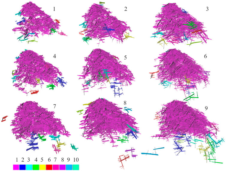
FIGURE 2. EDFMs representing uncertainty in fracture networks of the real carbonate reservoir. Color bar displays cluster size, with pink being the largest. Only cells belonging to the 10 largest clusters are shown; isolated cells are not displayed (figure from [16]).

In addition to the different DFNs, three model properties (fracture permeability, fracture pore volume, and matrix permeability) are varied through use of three categorical global multipliers (low, mid, and high) to capture their ranges of uncertainty. There is considerable variability in these properties, e.g., matrix permeabilities are on the order of 0.1 mD, while fracture permeabilities can be a factor of ${10}^6$ higher. Further, three discrete sets of relative permeabilities, (corresponding) capillary pressures, and rock compressibilities are used to represent uncertainty in the degree of water imbibition in the rock matrix as well as the impact of pore pressure/stress changes in the matrix and fractures. It should be noted that straight-line relative permeabilities, zero capillary pressure, and higher rock compressibilities are employed for fractures.

One model parameter, fracture pore volume, warrants additional elaboration because we will consider a value beyond its prior range when we apply DSI in Section 4. Fracture pore volume is a function of the heterogeneous distribution of fracture apertures, which themselves range from less than 1 mm to greater than 1 m. This latter value, which is much higher than that observed in typical fractured reservoirs, accounts for the existence of “caverns” in the carbonate formation. The fracture pore volume strongly impacts the amount of recoverable oil in the reservoir, so its value has a large effect on reservoir performance.

A total of $N_{\text{r}}=1850$ simulations are performed using the nine DFNs and low, mid and high values of the five uncertain parameters. A full-factorial experimental design with the nine DFNs and the set of uncertain parameters leads to an ensemble of 2,187 models. Because the simulations are challenging (due to the field-management logic and complex displacement physics), about 15% of the runs fail, which leaves us with 1850 successful runs. The models are represented on structured grids containing over 500,000 matrix cells, many of which contain embedded discrete fracture cells. An aggregation-based upscaling scheme that preserves network connectivity was further applied to the fracture cells, resulting in coarse EDFMs that contain ∼60,000 to 100,000 fracture cells.

The simulations capture three field stages: part of the primary depletion period with 11 existing producers (2.5 years), followed by a five-year water-injection pilot, and finally the large-scale full-field waterflood development that lasts for 17.5 years. Note that we did not consider the actual full depletion period (14 years) in order to have a more typical ratio of historical period (3,600 days) to forecast period (5,400 days). During the pilot period, two wells inject water at a target rate subject to a maximum bottom-hole pressure (BHP), while the existing producers operate at prescribed target oil rates subject to minimum BHP constraints. Injected water contains different tracers (referred to as A and B) that can be detected at nearby producers. Breakthrough time, for example, is one of several pilot indicators measured to assist in predicting future full-field waterflood performance (water breakthrough is expected to be controlled in part by fracture connectivity, which impacts sweep efficiency [17]). Three new producers will be introduced into the model during the pilot period.

At the start of the full-field development phase, an additional four injectors and three producers are drilled. The total water-injection rate for the six injectors is controlled to achieve a target voidage replacement ratio. The reservoir pressure drops below the bubble point at some point during this stage, leading to the evolution of free gas. The resulting three-phase flow is one of several simulation challenges. For example, the producers are subject to many other constraints such as tubing head pressure (controlled by flow tables as a proxy for surface network dependencies), as well as maximum gas/oil ratio and watercut due to plant-handling capacities for water and gas. As a result, wells are shut-in and revived frequently based on a complicated set of field-management rules. This leads to “spiky” well production and injection behavior, which in turn poses significant challenges for the parameterization procedures.

The flow simulations are also difficult because the reservoir models contain many stratigraphic layers that pinch-out, which can lead to small cells (especially fracture cells) that limit the time-step size. This is partly ameliorated by the EDFM gridding, which enforces a lower bound on fracture cell size, as well as by the upscaling. The overall workflow requires on average about 10 min per model for gridding and i/o, and 2.0 h for simulation (in parallel, with 16 processors on 64-bit LINUX clusters equipped with 2x AMD EPYC 7502 32-Core Processor with 512 GB of memory). The additional computational effort required by the DSI procedure (for parameterization and posterior sampling) is essentially negligible compared to that for generating the prior data realizations.

Reconstruction of Prior Data With PCA and RAE

Although our eventual goal is the use of the data parameterization treatments for data-space inversion, it is important to first assess the ability of the two methods to reconstruct new data realizations; i.e., prior data vectors not included in training. As is evident from the discussion in Section 2.2, ESMDA is applied to the latent variable $\mathit{\xi }$ generated from the parameterization process, and the initial guess for ${\mathit{\xi }}_{\text{post}}^{\text{PCA}}$ or ${\mathit{\xi }}_{\text{post}}^{\text{RAE}}$ is the associated prior $\mathit{\xi }$. Thus, the quality of the posterior predictions is likely to depend on the quality of the prior reconstruction.

In this study, we construct parameterizations and apply DSI only for selected field-wide and well-level QoI. Specifically, we model water injection rates (WIR) for the field and for pilot injectors I1 and I2, as well as the water production rates (WPR) and oil production rates (OPR) for the field and for four of the 14 producers (P1–P4). These producers are deemed to be the most promising for tracer detection during the pilot due to their proximity to I1 and I2. We also include the tracer A production rate (TAR) for the field and for wells P2 and P4, and the tracer B production rate (TBR) for the field and for wells P1 and P3. The final quantities considered are the static well pressures (SWP) for all injectors and producers. In total, there are 25 QoI, i. e, $N_{\text{QoI}}=25$. The simulation period is 9,000 days. We sample data every 180 days, which partially smooths the time-series data that result from the complex field management strategy. Thus the number of time steps $\left(N_{\text{t}}\right)$ is 50, and the length of the data vector ($N_{\text{f}}$) is 1,250.

We simulate a total of $N_{\text{r}}=1850$ prior model realizations. Of these, $N_{\text{train}}=1350$ data vectors, selected randomly from the full set, are used to construct the PCA basis matrix and for the training of the RAE model. The remaining $N_{\text{val}}=500$ data vectors are used for validation. Although these 500 realizations are not used for PCA basis construction or for RAE training, they are included in the set of prior data realizations used for DSI in Section 4 (meaning we have $N_{\text{r}}=1850$ prior samples).

We preserve 99% of the energy in the construction of the PCA basis matrix. This results in $N_{\text{l}}\approx 100$. The prior samples of ${\mathit{\xi }}^{\text{PCA}}$ are generated through application of ${\mathit{\xi }}_i^{\text{PCA}}={\text{Φ}}^T\left({\mathbf{d}}_i-{\overline{\mathbf{d}}}_{\text{prior}}\right)$, $i=\mathrm{1,2},\dots ,N_{\text{r}}$. We then reconstruct the prior data using the basis matrix and histogram transformation; i.e., ${\tilde{\mathbf{d}}}_i=h_T\left(\text{Φ}\left({\mathit{\xi }}_i^{\text{PCA}}+{\overline{\mathbf{d}}}_{\text{prior}}\right)\right)$. We set $N_{\text{l}}=100$ for the RAE latent space to maintain consistency with PCA. The Glorot uniform initializer [23] is applied to initialize the LSTM layer. The prior samples of the latent variables ${\mathit{\xi }}^{\text{RAE}}$ are generated with the encoder; i.e., ${\mathit{\xi }}_i^{\text{RAE}}=f_e\left({\text{d}}_i;W_e\right)$, $i=\mathrm{1,2},\dots ,N_{\text{r}}$. Prior-data reconstruction is then accomplished by the decoder, ${\tilde{\mathbf{d}}}_i=f_d\left({\mathit{\xi }}_i^{\text{RAE}};W_d\right)$, $i=\mathrm{1,2},\dots ,N_{\text{r}}$. In all results shown in this work, we normalize the time-series data using the maximum value of the corresponding field-wide quantity.

Before considering prior-data reconstruction, we present results for RAE training and testing performance. The evolution of RAE training and testing error (RMSE is defined in Eq. 10) with varying numbers of epochs, for $N_{\text{train}}=1350$ and training/testing split ratio of around 4.5/1, is shown in Figure 3A. Beyond around 400 epochs, we see the training error continue to generally decrease (though there are fluctuations), while the testing error has plateaued. From this plot we conclude that 500 epochs is sufficient for training, and this is the value used in this work.

FIGURE 3

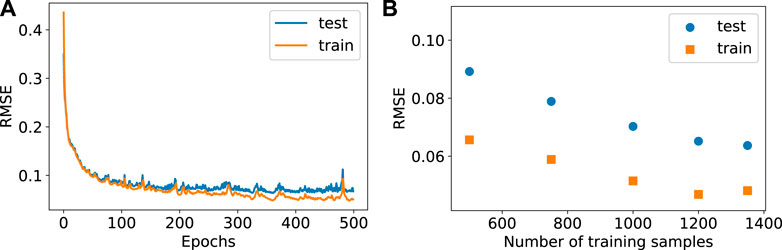
FIGURE 3. RAE error evolution during training and RAE error with different numbers of training samples.

Figure 3B shows the training and testing RMSE, with different numbers of training samples, at the end of 500 epochs. Note “training samples” refers to both data realizations used for the actual loss function minimization and data realizations used for testing during the training procedure. Here we again use a training/testing split ratio of around 4.5/1. Increasing the number of training samples generally decreases the training and testing RMSE, as expected, though the results approach a plateau by $N_{\text{train}}=1350$, which is the value used in this study. For $N_{\text{train}}=1350$, 1,100 samples are used for loss function minimization and 250 samples are used for testing.

Results for the reconstruction of prior data realizations are now presented. We show results drawn from the set of $N_{\text{val}}=500$ validation cases. For visual clarity, we display results for 50 cases, randomly selected from the full set of 500. As explained earlier, these data realizations are not used in the training process. Figures 4 and 5 display prior simulation results (gray curves in the left column), PCA with histogram transformation–referred to as PCA+HT–reconstructions (blue curves in the middle column), and RAE reconstructions (black curves in the right column). These results are for primary quantities, meaning that these QoI appear directly in the $\text{d}$ vector. Results in Figure 4 are for field-wide quantities (water injection and production rates and tracer A production rate), while those in Figure 5 are for well P4 (oil, water and tracer A production rates). We present quantities that are of particular relevance to the waterflood pilot and full-field development in question, even though many others, such as gas/oil ratio, may also display interesting behavior. The reconstructions are for data realizations that correspond to the 50 curves shown for prior simulation results in the left column.

FIGURE 4

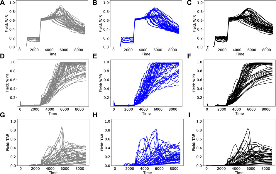
FIGURE 4. Prior simulation results (left column), PCA+HT reconstructions (middle column) and RAE reconstructions (right column) for field-wide quantities (A)–(C) field-wide water injection rate (D)–(F) field-wide water production rate (G)–(I) field-wide tracer A production rate.

FIGURE 5

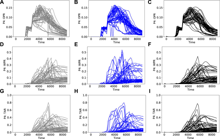
FIGURE 5. Prior simulation results (left column), PCA+HT reconstructions (middle column) and RAE reconstructions (right column) for well P4 quantities (A)–(C) P4 oil production rate (D)–(F) P4 water production rate (G)–(I) P4 tracer A rate.

Figure 4 shows the clear ramp-up of field water injection rate as more injectors come online after the end of the pilot (around 2,700 days). The corresponding rise in water production rate is also apparent. Eventually, the field water injection rate drops. This occurs after the field liquid production rate reaches a peak, in accordance with the voidage-replacement-ratio specification (required to be less than 1). In Figure 5, we see that, in some cases, P4 tracer A production rate increases and then decreases. This is due to dilution from tracer-free water from injectors that are drilled after the pilot ends. In other cases, where I1 remains the main source of water, the P4 tracer A production rate continually increases.

The simulation results are complex due to frequent changes in well operations resulting from the field management logic. Abrupt variations in the reference simulation results are evident in many of the curves, particularly in Figures 5D,G (and to some extent in Figure 4G). The PCA+HT reconstruction results are in general agreement with the prior simulation results, but they do show noticeable overprediction in some cases, at around 3,000–5,000 days, in Figure 4H and Figures 5E,H. Some higher-frequency oscillation compared to the reference results, particularly in Figure 4E and Figure 5E, is also apparent. These oscillations occur because, as discussed previously, time correlations are not maintained with this approach.

The RAE reconstructions in Figures 4 and 5 are in better visual agreement with the reference prior results than the PCA+HT reconstructions. More specifically, the overprediction and oscillatory behavior evident in some of the PCA+HT results does not occur in the RAE reconstructions (e.g. compare Figures 5E,F). Interestingly, the RAE results tend to be slightly smoother than the reference results. Although this may actually be desirable in some settings, such smoothing can in general be mitigated by increasing the latent-space dimension and/or using a more complex network.

We now assess the performance of the reconstructions for derived quantities. By derived quantity, we mean QoI not directly included in $\text{d}$, which must be computed from the results for primary quantities. We consider cumulative injection and production, liquid production rate (sum of oil and water production rates), and water cut for producers (water rate divided by liquid production rate). To provide accurate derived QoI, the parameterization must capture the correlations between primary quantities.

Figure 6 displays prior simulation results and reconstruction results for P4 water cut, P4 liquid production rate, and field-wide liquid production rate. In Figures 6B,E, we see a high degree of nonphysical oscillations in the PCA+HT results. Capturing the correct behavior of derived quantities such as water cut is important because it has implications for the field development plan (e.g. on the timing for additional water-handling capacity). The RAE reconstructions, by contrast, display close agreement with the reference prior simulation results. This suggests that, consistent with our earlier findings for much simpler systems [5], the RAE parameterization is able to capture correlations more accurately than the PCA+HT treatment for this complicated case.

FIGURE 6

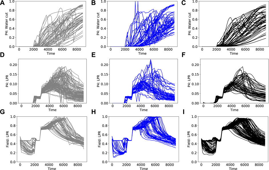
FIGURE 6. Prior simulation results (left column), PCA+HT reconstructions (middle column), RAE reconstructions (right column) for derived quantities (A)–(C) P4 water cut (D)–(F) P4 liquid production rate (G)–(I) field-wide liquid production rate.

We now further assess the ability of the two parameterizations to capture correlations in the prior simulation data. This will be evaluated both visually, through cross-plots, and in terms of the covariance between sets of quantities. For two quantities x and y, covariance is given by

$\text{Cov}\left(x,y\right)=E\left[\left(x-{\mu }_x\right)\left(y-{\mu }_y\right)\right],(15)$

where ${\mu }_x$ and ${\mu }_y$ denote the mean values of x and y. We compute the covariance between two quantities at each time step to evaluate the time evolution.

Figures 7–10 show cross-plots for different primary and derived quantities at 8,280 days, along with the covariance between the two time series. In these plots, results for all $N_{\text{val}}=500$ validation cases are displayed. Figure 7 shows results for P4 water production rate and tracer A production rate. The gray points in Figure 7A are the prior simulation results, the blue points in Figure 7B are from the PCA+HT reconstruction, and the black points in Figure 7C are from the RAE reconstruction. We observe an approximately linear relationship between tracer A production and water production for producer P4. This behavior is expected because the injected tracers partition into the water phase. The PCA+HT reconstruction overestimates the scatter in this relationship, while the RAE reconstruction is in close visual agreement with the prior. The covariance plot in Figure 7D also demonstrates that the RAE reconstruction provides a closer match to the prior. The small (y-axis) values on this and subsequent covariance plots result from the data normalization.

FIGURE 7

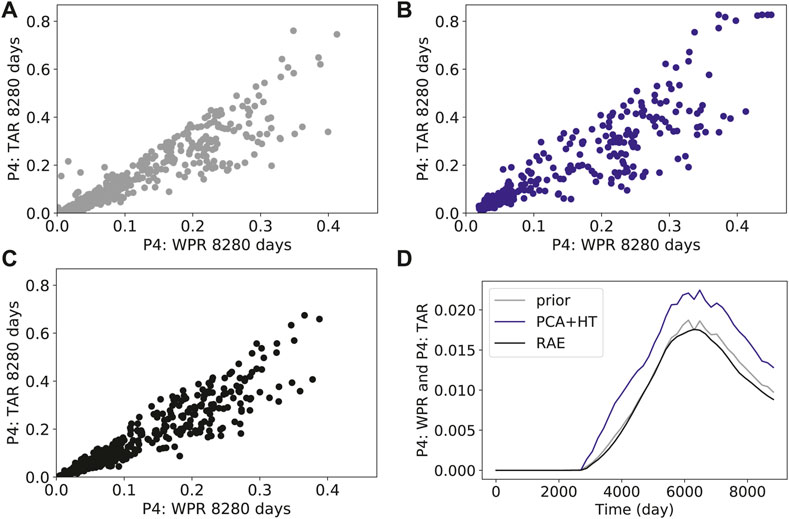
FIGURE 7. Cross-plots and covariance curves for tracer A production rate in well P4 and water production rate in well P4 (A) prior simulation results (B) PCA+HT reconstructions (C) RAE reconstructions (D) covariance.

Figures 8–10 present cross-plots and covariance curves for three different sets of derived quantities. Figure 8 displays results for cumulative production of tracer B at well P1 against cumulative water production for well P1, Figure 9 shows results for well P4 water cut against well P4 oil production rate, and Figure 10 presents results for field-wide cumulative liquid production against field-wide cumulative water injection. The linear trends evident in Figure 10 are reflective of the voidage-replacement control in field-wide injection, while the separation into three clusters reflects the three different rock-compressibility curves considered (see Section 3.1). In all cases, we observe better agreement with the reference simulation results with the RAE reconstruction than with the PCA+HT reconstruction. This is evident in all of the covariance plots, and in the ranges and character of the cross-plots. For example, the range of the prior is better captured in Figure 8C than in Figure 8B, and the continuity and linear character of the upper cluster of points is better captured in Figure 10C than in Figure 10B.

FIGURE 8

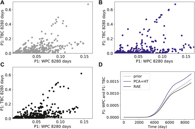
FIGURE 8. Cross-plots and covariance curves for tracer B cumulative production in well P1 and cumulative water production in well P1 (A) prior simulation results (B) PCA+HT reconstructions (C) RAE reconstructions (D) covariance.

FIGURE 9

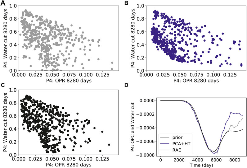
FIGURE 9. Cross-plots and covariance curves for water cut in well P4 and oil production rate in well P4 (A) prior simulation results (B) PCA+HT reconstructions (C) RAE reconstructions (D) covariance.

FIGURE 10

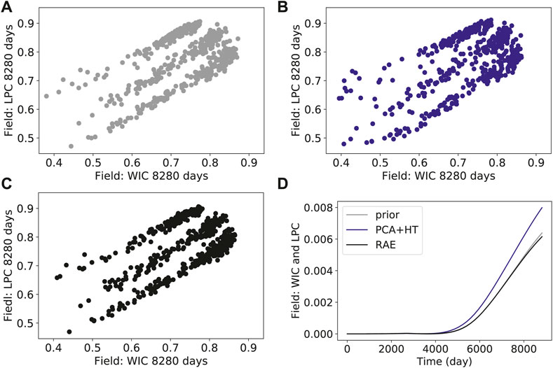
FIGURE 10. Cross-plots and covariance curves for field-wide cumulative liquid production and field-wide cumulative water injection (A) prior simulation results (B) PCA+HT reconstructions (C) RAE reconstructions (D) covariance.

Posterior Predictions Using DSI

We now assess DSI posterior results using the two parameterization procedures. Although the reservoir models considered in this study are used for actual field modeling, the field data are confidential and thus not available for use in our assessments. We therefore utilize simulated data as described earlier. The “synthetic” nature of the data is partially mitigated through the addition of random noise (see Eq. 11). To further “stress-test” the DSI framework, in the first assessment (in Section 4.1) we generate synthetic data from a true model that is characterized by a key model parameter that is outside the prior range. Specifically, we assign this true model a fracture pore volume that is 1/2 of the lowest value used in the prior ensemble. Importantly, although the model itself is outside the prior, the data still fall within the prior data range. Because the prior range in this work is much broader than that often considered in history matching studies (recall we consider nine DFN realizations coupled with wide ranges for other key parameters), the requirement that the data lie within the prior range is not an overly limiting constraint.

We note finally that a general correspondence between the observed data and the prior simulation results should be established in an initial prior-validation step. This can be accomplished, for example, through use of the Mahalanobis distance, as described within a DSI context in [24]. If the data fall well outside the prior range, then the prior must be extended before DSI, or any other inversion procedure, is applied. Although important in practice, we view the prior-validation step as outside the scope of this study.

In all cases considered, the observed data (generated from simulation results for the true model with noise added, as described in Section 2.2) include values for all primary quantities at 900, 1800, 2,700 and 3,600 days. The number of observed data values ($N_{\text{hm}}$) is 100 and measurement error is prescribed to be 5% of the true value for all quantities. As noted earlier, we have a total of $N_{\text{r}}=1850$ prior data realizations. ESMDA is applied $N_{\text{a}}=10$ times to generate $N_{\text{r}}=1850$ posterior samples.

In Section 4.1, we present detailed DSI results, with both parameterizations, for true model 1. Then, in Section 4.2, we consider the representation of DSI posterior data predictions (for true model 1) in terms of linear combinations of prior data realizations. In Section 4.3, DSI performance for five additional true models is assessed through use of coverage probability metrics.

DSI Results for True Model 1

As indicated above, the fracture pore volume for true model 1 lies outside of the prior range, while the other model parameters fall within the prior range. Posterior results for three field-wide primary quantities–water injection rate, water production rate, and tracer A production rate–are shown in Figure 11. Additional results for primary quantities for well P4–oil production rate, water production rate, and tracer A production rate–appear in Figure 12. In the figures, the gray-shaded regions indicate the ${\text{P}}_{10}$–${\text{P}}_{90}$ interval for the prior simulation results, where ${\text{P}}_{10}$ and ${\text{P}}_{90}$ denote the 10th and 90th percentile values of the data variable at each time step (results at different time steps in general correspond to different data realizations). The red curves show the true data, generated via simulation of the true model. The red points show the observed data, which include random measurement error. The lower, middle and upper black curves represent the ${\text{P}}_{10}$, ${\text{P}}_{50}$ and ${\text{P}}_{90}$ posterior results. The black curves in the left columns of Figures 11 and 12 depict the PCA+HT DSI posterior results, and those in the right columns display RAE-based DSI results. The true field-wide water injection and production rates (Figure 11) are near the low end of the prior distribution due to the low fracture pore volume.

FIGURE 11

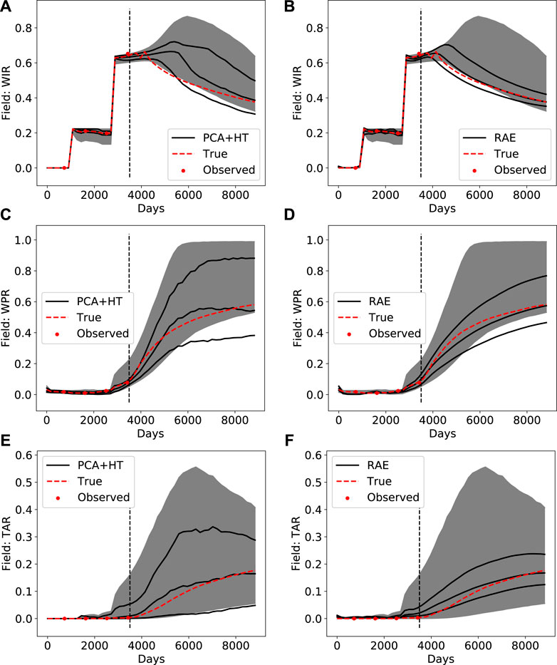
FIGURE 11. Posterior DSI results using PCA+HT parameterization (left column) and RAE-based parameterization (right column) for (A) and (B) field-wide water injection rate (C) and (D) field-wide water production rate (E) and (F) field-wide tracer A production rate.

FIGURE 12

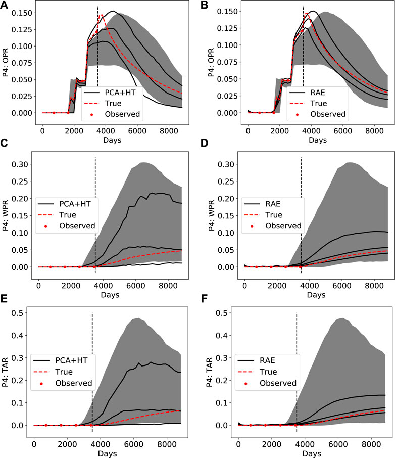
FIGURE 12. Posterior DSI results using PCA+HT parameterization (left column) and RAE-based parameterization (right column) for (A) and (B) P4 oil production rate (C) and (D) P4 water production rate (E) and (F) P4 tracer A rate.

We see that more uncertainty reduction is accomplished using RAE-based DSI than with the PCA+HT treatment. This is evident through comparison of all posterior results in Figure 11 and Figure 12. The general shape of the true response is also better captured by RAE, as can be seen by comparing Figure 11B to Figure 11A, and Figure 12B to Figure 12A. The true response is within the ${\text{P}}_{10}$–${\text{P}}_{90}$ posterior uncertainty range for most time steps, for all QoI, for both sets of DSI results. We will presented coverage probability results in Section 4.3, which will enable further comparisons between posterior predictions for the two parameterization procedures.

Figure 13 displays posterior results for three derived quantities–well P4 water cut, well P4 liquid production rate, and field-wide liquid production rate. We again see a greater amount of uncertainty reduction with RAE-based DSI than with the PCA+HT treatment. This is particularly noticeable in the liquid production rate results for both well P4 and for the full field. Note that, because the true model is outside of the prior, the field-wide liquid production rates in Figures 13E,F are below the ${\text{P}}_{10}$ prior results. Both the PCA+HT and RAE treatments are, however, still able to provide posterior predictions that appear reasonable.

FIGURE 13

FIGURE 13. Posterior DSI results using PCA+HT parameterization (left column) and RAE-based parameterization (right column) for derived quantities (A) and (B) P4 water cut (C) and (D) P4 liquid production rate (E) and (F) field-wide liquid production rate.

Next, we consider correlations between posterior quantities for the two parameterization methods. Figures 14 and 15 display cross-plots for primary and derived quantities. The corresponding prior results appear in Figures 7–10. The gray points in the left column display the prior simulation results (for all 1850 prior samples), the blue points in the middle column show DSI results using the PCA+HT parameterization, and the black points in the right column are DSI results using the RAE-based parameterization. The gray points in the background in the middle and right columns are the prior simulation results (these points are the same as in the plots in the left column). The red points depict the true data.

FIGURE 14

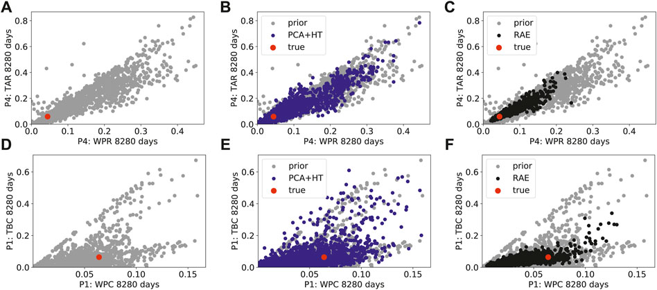
FIGURE 14. Cross-plots for prior simulation results (left column), posterior DSI results using PCA+HT parameterization (middle column) and posterior DSI results using RAE-based parameterization (right column) (A)–(C) P4 tracer A production rate against P4 water production rate (D)–(F) P1 tracer B cumulative production against P1 cumulative water production.

FIGURE 15

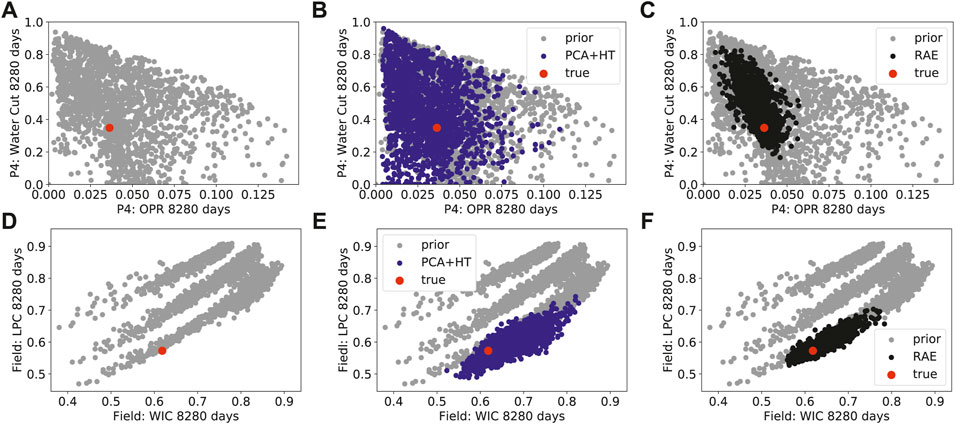
FIGURE 15. Cross-plots for prior simulation results (left column), posterior DSI results using PCA+HT parameterization (middle column) and posterior DSI results using RAE-based parameterization (right column) (A)–(C) P4 water cut against P4 oil production rate (D)–(F) field-wide cumulative liquid production against field-wide cumulative water injection.

These figures again demonstrate the increased uncertainty reduction achieved using the RAE-based parameterization in DSI relative to that using the PCA+HT parameterization. In Figure 14B, with the true data point falling near the (lower-left) edge of the prior data, we see very little uncertainty reduction with PCA+HT. In the RAE-based result (Figure 14C), by contrast, a reasonable degree of uncertainty reduction is achieved. Similar observations can be made between Figures 14E,F, and between Figures 15B,C.

In this assessment, it is important to capture correlations between key data quantities to obtain accurate estimates of the expected uncertainty reduction in the main QoI. For example, by collecting indicator data such as P4 tracer production rate (Figures 12E,F), we can potentially gain insight regarding future P4 oil production (Figures 12A,B). In particular, for P4 water production rate, we see more uncertainty reduction, and a shift toward lower predicted production rates, with RAE-based DSI (Figures 12C,D). This shift is likely due, at least in part, to the impact of data types other than historical P4 oil rate. Relationships such as that between tracer production rates and field oil/water rates will be used to select the appropriate pilot surveillance plan and to interpret pilot data. This in turn will enable us to evaluate the cost-effectiveness of expanding the waterflood to the full field. More details on the interpretation of pilot data (and related issues) are provided by [17].

Although the posterior DSI results presented in this section (along with the prior reconstruction results shown earlier) suggest that the RAE-based parameterization outperforms the PCA+HT parameterization, we cannot draw definitive conclusions on this point in the absence of a clear set of reference posterior results. In our earlier study [5], we applied rejection sampling to provide reference posterior results. Comparisons with these results indeed demonstrated that the RAE-based parameterization provided posterior predictions of high accuracy and that it outperformed the PCA+HT treatment. The rejection sampling results required $O\left({10}^6\right)$ simulation runs, which was manageable for the much simpler cases in [5]. However, for the models considered in this work (and the larger number of observations), it would be extremely time-consuming to perform the runs required for rejection sampling. In Section 4.3 we will proceed in a more indirect manner, by considering coverage probability for multiple “true” models.

Prior Realization Selection

In some settings, it may be useful to identify a subset of prior models that can be used to explain the DSI posterior responses. These “most-relevant” prior models could then be used for other reservoir management applications. This identification is challenging, however, because each posterior data realization corresponds to a different set of prior realizations. Nonetheless, if the data are highly informative, we might expect that posterior data realizations can be expressed in terms of linear combinations of a relatively small set of prior realizations.

To quantify the relationship between prior and posterior data realizations for true model 1, we now reconstruct each of the $N_{\text{r}}$ DSI (with the RAE-based parameterization) posterior samples as a linear combination of the $N_{\text{r}}$ prior realizations. For each posterior data sample ${\left({\mathbf{d}}_{\text{post}}\right)}_i,i=\mathrm{1,2},\dots ,N_{\text{r}}$, we apply Lasso regression [25] to determine the weights $w_{i,j}$ associated with each prior realization ${\left({\mathbf{d}}_{\text{prior}}\right)}_j,j=\mathrm{1,2},\dots ,N_{\text{r}}$. The goal of Lasso regression is the minimization of the mismatch $S_L$, given by

$S_L={\Vert {\left({\mathbf{d}}_{\text{post}}\right)}_i-{\displaystyle \sum _{j=1}^{N_{\text{r}}}{w}_{i,j}{\left({\mathbf{d}}_{\text{prior}}\right)}_j}\Vert }_2^2+\lambda {\displaystyle \sum _{j=1}^{N_{\text{r}}}\left|w_{i,j}\right|}\text{.}(16)$

Here the ${\text{L}}_1$ norm of the weights is applied for regularization, with λ representing the tuning parameter that balances prediction accuracy with the number of prior realizations used in the approximation of each ${\left({\mathbf{d}}_{\text{post}}\right)}_i$. All weights are specified to be positive, which enforces physically meaningful interpolations. By combining all of the prior realizations used for the full set of posterior samples, a subset of prior realizations that can be applied to construct the posterior statistics is identified. We consider different cutoff values for the $w_{i,j}$ coefficients (larger cutoffs lead to a smaller number of prior realizations needed for the reconstructions).

Figure 16 shows the posterior results (for primary quantities) considered in this assessment. Results for 50 posterior realizations are displayed, but all 1850 are considered in the results that follow. Table 1 presents the number of prior realizations needed to reconstruct the $N_{\text{r}}=1850$ posterior samples for a range of cutoff values. We see that, even for a cutoff value of 0.1 (which is rather large), 135 prior realizations are needed. Significantly more prior realizations are required to fully characterize the posterior results with smaller cutoff values.

FIGURE 16

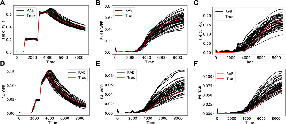
FIGURE 16. Posterior data realizations for primary quantities (A) field-wide water injection rate (B) field-wide water production rate (C) field-wide tracer A production rate (D) P4 oil production rate (E) P4 water production rate (F) P4 tracer A rate.

TABLE 1

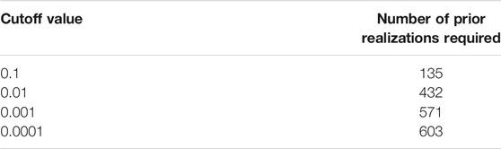
TABLE 1. Number of prior realizations required to construct all posterior samples for different coefficient cutoff values.

The results in Table 1 clearly indicate that DSI posterior results cannot be expressed in terms of a small number of prior data realizations that fall near the observations. It should be noted, however, that particular responses (e.g. one of the curves in Figure 16) may be represented, through use of Eq. 16, in terms of $\sim 10$ or even fewer prior realizations. Thus, for the ${\text{P}}_{50}$ oil rate for well P4, for example, we can identify a small number of model realizations that can be used to capture the DSI response. This could be useful both for enhancing the “explainability” of DSI results and for subsequent reservoir management applications where models are needed, such as well placement optimization.

DSI Results for Multiple True Models

In our final assessment, we construct posterior DSI results using both parameterization procedures for a set of five additional true models. For conciseness, in these results we present only a single metric, coverage probability (CP). The coverage probability is defined as the fraction of the true data that fall in a specific range of the DSI posterior results, i.e.,

$\text{CP}=\frac{N_{\text{c}}}{N_{\text{f}}}\text{,}(17)$

where $N_{\text{c}}$ denotes the number of posterior data variables that fall within the specified range. Here we consider three uncertainty ranges for CP, specifically the ${\text{P}}_{10}$–${\text{P}}_{90}$, ${\text{P}}_5$–${\text{P}}_{95}$, and ${\text{P}}_{25}$–${\text{P}}_{75}$ intervals. The target values of CP for these intervals are 0.8, 0.9, and 0.5. Higher CP values indicate the overestimation of posterior uncertainty and lower values indicate underestimation.

The five new true models (denoted true models 2–6) are random realizations not included in the set of prior models, but the values of all model parameters are in the prior range (this was not the case for true model 1 considered in Sections 4.1 and 4.2). We construct posterior DSI results precisely as in Section 4.1. Results for coverage probability are presented in Figure 17. For the ${\text{P}}_{10}$–${\text{P}}_{90}$ range (Figure 17A), DSI results using the PCA+HT parameterization (blue bars, mean value of 0.859) consistently overpredict the target value of 0.8, while those using the RAE-based parameterization (orange bars, mean value of 0.810) are closer to the target value. Similar observations apply for the other intervals. Specifically the average CP values for the PCA+HT posteriors are 0.927 for the ${\text{P}}_5$–${\text{P}}_{95}$ interval and 0.643 for ${\text{P}}_{25}$–${\text{P}}_{75}$ interval, while those using RAE are 0.901 and 0.539.

FIGURE 17

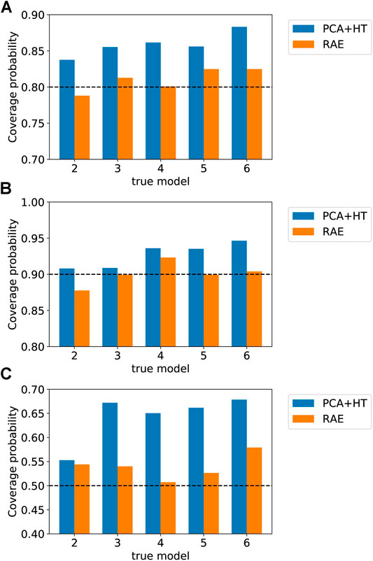
FIGURE 17. Coverage probability (CP) for five new true models (A) CP for ${\text{P}}_{10}$–${\text{P}}_{90}$ interval (B) CP for ${\text{P}}_5$–${\text{P}}_{95}$ interval (C) CP for ${\text{P}}_{25}$–${\text{P}}_{75}$ interval. Target values indicated by the dashed lines.

These results are consistent with our observation in Section 4.1 that the PCA+HT treatment generally corresponds to higher DSI posterior uncertainty. This is likely due to the fact that the PCA+HT parameterization does not fully capture correlations between different QoI. As a result, measurements for a particular quantity at a particular time may not lead to the correct level of uncertainty reduction for other quantities. Because the RAE-based parameterization better captures correlations in the data, it provides more accurate estimates for posterior uncertainty.

Concluding Remarks

In this paper, we applied recently developed data-space inversion treatments for a naturally fractured reservoir. These treatments involve the use of a recurrent autoencoder (RAE) for the parameterization of well-level and field-level time series of interest. The RAE utilizes a long short-term memory (LSTM) architecture, and the resulting network is able to capture the physical behavior and correlations in the time-series data. The overall RAE-based DSI procedure, introduced in [5], applies ESMDA for posterior sampling, as originally suggested (within a DSI context) by [4]. The examples considered in [5] were somewhat idealized, however. The (real) case considered here, by contrast, is much more complicated and includes multiple 3D fracture scenarios, three-phase flow, tracer injection and production, and detailed well and field management logic that forces frequent well shut-in and reopening. A total of 1850 prior data vectors (time series) were constructed though simulation of prior geomodels. This is the time-consuming step in DSI.

In addition to the RAE-based parameterization, we also considered the use of a parameterization based on PCA and histogram transformation [2]. We first assessed the two parameterization procedures in terms of their ability to reconstruct time-series data for realizations not included in the training set. The RAE-based parameterization outperformed the PCA-based method for these time-series reconstructions, and was shown to better capture correlations in the prior data. Superior RAE performance was observed both for primary quantities (data variables included in the data vector) and for derived quantities (which are not directly included in the data vector).

Posterior DSI results (${\text{P}}_{10}$, ${\text{P}}_{50}$, ${\text{P}}_{90}$ time series and cross-plots at particular times) using the two parameterizations were then presented. A greater degree of uncertainty reduction was achieved with the RAE-based parameterization. We do not have reference results for posterior uncertainty because rigorous approaches such as rejection sampling are intractable for this challenging field case. Nonetheless, we believe the RAE-based results to be the more accurate because of their greater accuracy in prior reconstruction and due to the limited amount of uncertainty reduction observed with the PCA approach in cases where the data appear to be informative. This speculation is somewhat corroborated through the consideration of five additional “true” models, for which we computed coverage probabilities over three different uncertainty intervals. These results indicated that the posterior uncertainty range was more accurately quantified by the RAE-based procedure than by the PCA approach.

There are many interesting directions that should be pursued in future work. In the current RAE method, the latent space provided by the encoder is close to (but not precisely) multivariate-Gaussian distributed. It will be useful to develop and test other encoding treatments, e.g., variational autoencoder or generative adversarial network, in an attempt to achieve (precise) multi-Gaussian latent variables which, upon decoding, still provide highly accurate reconstructions of the prior data. If we are able to accomplish this, we could apply the network to provide synthetic prior data realizations; i.e., realistic data realizations, with correct correlations between data variables, that do not require numerical simulation. Further investigation of the selection of the most-relevant prior realizations, using the approach presented in Section 4.2, should also be performed. It will additionally be of interest to combine model-based inversion with data-space inversion by introducing parameterizations that couple data and model parameters. Then, by conducting data assimilation in the joint space, we could efficiently generate posterior models along with posterior data realizations.

Data Availability Statement

The datasets presented in this article are not readily available because the data are proprietary to Chevron. Inquiries regarding the data should be directed to Robin Hui, robin.hui@chevron.com.

Author Contributions

SJ: Conceptualization, development of DSI and RAE methodologies, software development, generation and interpretation of DSI results, writing. M-HH: Conceptualization, generation of full-order simulation results, interpretation of results, writing. LD: Conceptualization, interpretation of results, writing and editing, funding acquisition.

Funding

Financial support was provided by Chevron Technical Center and by the industrial affiliates of the Stanford Smart Fields Consortium.

Conflict of Interest

Author M-HH is employed by Chevron Technical Center. SJ and LJD declare that they received funding from Chevron Technical Center for this study. Beyond M-HH's direct involvement as a co-author, the funder was not involved in the study design, the collection, analysis, and interpretation of data, the writing of this article, or the decision to submit it for publication.

The remaining authors declare that the research was conducted in the absence of any commercial or financial relationships that could be construed as a potential conflict of interest.

References

1. Sun, W, and Durlofsky, LJ. A New Data-Space Inversion Procedure for Efficient Uncertainty Quantification in Subsurface Flow Problems. Math Geosci (2017) 49:679–715. doi:10.1007/s11004-016-9672-8

CrossRef Full Text | Google Scholar

2. Sun, W, Hui, M-H, and Durlofsky, LJ. Production Forecasting and Uncertainty Quantification for Naturally Fractured Reservoirs Using a New Data-Space Inversion Procedure. Comput Geosci (2017) 21:1443–58. doi:10.1007/s10596-017-9633-4

CrossRef Full Text | Google Scholar

3. Jiang, S, Sun, W, and Durlofsky, LJ. A Data-Space Inversion Procedure for Well Control Optimization and Closed-Loop Reservoir Management. Comput Geosci (2020) 24:361–79. doi:10.1007/s10596-019-09853-4

CrossRef Full Text | Google Scholar

4. Lima, MM, Emerick, AA, and Ortiz, CEP. Data-Space Inversion with Ensemble Smoother. Comput Geosci (2020) 24:1179–200. doi:10.1007/s10596-020-09933-w

CrossRef Full Text | Google Scholar

5. Jiang, S, and Durlofsky, LJ. Data-Space Inversion Using a Recurrent Autoencoder for Time-Series Parameterization. Comput Geosci (2021) 25:411–32. doi:10.1007/s10596-020-10014-1

CrossRef Full Text | Google Scholar

6. Scheidt, C, Renard, P, and Caers, J. Prediction-focused Subsurface Modeling: Investigating the Need for Accuracy in Flow-Based Inverse Modeling. Math Geosci (2015) 47:173–91. doi:10.1007/s11004-014-9521-6

CrossRef Full Text | Google Scholar

7. Satija, A, and Caers, J. Direct Forecasting of Subsurface Flow Response from Non-linear Dynamic Data by Linear Least-Squares in Canonical Functional Principal Component Space. Adv Water Resour (2015) 77:69–81. doi:10.1016/j.advwatres.2015.01.002

CrossRef Full Text | Google Scholar

8. Satija, A, Scheidt, C, Li, L, and Caers, J. Direct Forecasting of Reservoir Performance Using Production Data without History Matching. Comput Geosci (2017) 21:315–33. doi:10.1007/s10596-017-9614-7

CrossRef Full Text | Google Scholar

9. Park, J, and Caers, J. Direct Forecasting of Global and Spatial Model Parameters from Dynamic Data. Comput Geosciences (2020) 143:104567. doi:10.1016/j.cageo.2020.104567

CrossRef Full Text | Google Scholar

10. Jeong, H, Sun, AY, Lee, J, and Min, B. A Learning-Based Data-Driven Forecast Approach for Predicting Future Reservoir Performance. Adv Water Resour (2018) 118:95–109. doi:10.1016/j.advwatres.2018.05.015

CrossRef Full Text | Google Scholar

11. He, J, Tanaka, S, Wen, XH, and Kamath, J. Rapid S-Curve Update Using Ensemble Variance Analysis with Model Validation. In: SPE Western Regional Meeting; Bakersfield, CA, United States: Society of Petroleum Engineers (2017).

Google Scholar

12. He, J, Sun, W, and Wen, XH. Rapid Forecast Calibration Using Nonlinear Simulation Regression with Localization. In: SPE Reservoir Simulation Conference; Galveston, TX, United States: Society of Petroleum Engineers (2019).

Google Scholar

13. Grana, D, Passos de Figueiredo, L, and Azevedo, L. Uncertainty Quantification in Bayesian Inverse Problems with Model and Data Dimension Reduction. Geophysics (2019) 84:M15–M24. doi:10.1190/geo2019-0222.1

CrossRef Full Text | Google Scholar

14. Mohd Razak, S, and Jafarpour, B. Rapid Production Forecasting with Geologically-Informed Auto-Regressive Models: Application to Volve Benchmark Model. In: SPE Annual Technical Conference and ExhibitionSociety of Petroleum Engineers (2020).

Google Scholar

15. Yang, S, Yang, D, Chen, J, and Zhao, B. Real-time Reservoir Operation Using Recurrent Neural Networks and Inflow Forecast from a Distributed Hydrological Model. J Hydrol (2019) 579:124229. doi:10.1016/j.jhydrol.2019.124229

CrossRef Full Text | Google Scholar

16. Hui, MH, Dufour, G, Vitel, S, Muron, P, Tavakoli, R, Rousset, M, et al. A Robust Embedded Discrete Fracture Modeling Workflow for Simulating Complex Processes in Field-Scale Fractured Reservoirs. In: SPE Reservoir Simulation Conference; Galveston, TX, United States: Society of Petroleum Engineers (2019).

Google Scholar

17. He, J, and Hui, M. IOR Pilot Evaluation in Brown-Field Fractured Reservoir Using Data Analytics of Reservoir Simulation Results. In: SPE Reservoir Simulation Conference; Galveston, TX, United States: Society of Petroleum Engineers (2019).

Google Scholar

18. Hochreiter, S, and Schmidhuber, J. Long Short-Term Memory. Neural Comput (1997) 9:1735–80. doi:10.1162/neco.1997.9.8.1735

PubMed Abstract | CrossRef Full Text | Google Scholar

19. Kingma, DP, and Ba, J. Adam: a Method for Stochastic Optimization. arXiv (2014) [Epub ahead of print]. Available at: https://arxiv.org/abs/1412.6980.

Google Scholar

20. Emerick, AA, and Reynolds, AC. Ensemble Smoother with Multiple Data Assimilation. Comput Geosciences (2013) 55:3–15. doi:10.1016/j.cageo.2012.03.011

CrossRef Full Text | Google Scholar

21. Evensen, G. Sampling Strategies and Square Root Analysis Schemes for the EnKF. Ocean Dyn (2004) 54:539–60. doi:10.1007/s10236-004-0099-2

CrossRef Full Text | Google Scholar

22. Emerick, AA, and Reynolds, AC. History Matching Time-Lapse Seismic Data Using the Ensemble Kalman Filter with Multiple Data Assimilations. Comput Geosci (2012) 16:639–59. doi:10.1007/s10596-012-9275-5

CrossRef Full Text | Google Scholar

23. Glorot, X, and Bengio, Y. Understanding the Difficulty of Training Deep Feedforward Neural Networks. In: Proceedings of the Thirteenth International Conference on Artificial Intelligence and Statistics (JMLR Workshop and Conference Proceedings) (2010). p. 249–56.

Google Scholar

24. Sun, W, and Durlofsky, LJ. Data-Space Approaches for Uncertainty Quantification of CO₂ Plume Location in Geological Carbon Storage. Adv Water Resour (2019) 123:234–55. doi:10.1016/j.advwatres.2018.10.028

CrossRef Full Text | Google Scholar

25. Tibshirani, R. Regression Shrinkage and Selection via the LASSO. J R Stat Soc Ser B (Methodological) (1996) 58:267–88. doi:10.1111/j.2517-6161.1996.tb02080.x

CrossRef Full Text | Google Scholar