Ensemble Transform Kalman Incremental Smoother and Its Application to Data Assimilation and Prediction

Introduction

Data assimilation (DA) seeks to optimally combine the information of observations and short-range model forecast to estimate the optimal analysis, which is closest to the real atmosphere [1]. The analysis serves as the initial condition for numerical weather prediction (NWP), and thus, its accuracy plays an important role in improving NWP. During the recent decades, the ensemble Kalman filter (EnKF; [2, 3]) has become a popular choice to establish a stand-alone or component of hybrid DA systems due to its ability to use flow-dependent background errors so that observations can be assimilated effectively to provide flow-dependent corrections.

Although the advancement of DA has proven to be a milestone to improve numerical weather/climate prediction, it is known that DA could also bring unwelcome side effects. Corrections not only eliminate errors but also may introduce unrealistic signals into the model state and induce model shock as the forecasts are initialized. This problem can result in spin-down, such as unrealistic heavy rain after initialization or unrealistic gravity wave propagation induced by the imbalanced model state, and can degrade the forecast skill and computational stability. Specifically, the structure of background error covariance plays an important role in providing analysis increment, affecting the balance of the initial model state. The improper representation of background error covariance is a major source of generating dynamical imbalance and model shock [4]. Under the framework of the EnKF, the issues of model shock and imbalance are also related to the use of covariance localization ([5, 6], 34) to avoid sampling errors causing spurious corrections at far distance. The covariance localization is generally done with a chosen distance-dependent function [7] without the dynamical dependency and will distort the structure of the corrections [8]. Applying a distance-dependent localization can break the geostrophic balance [5], and the choice of localization radius is an issue of trade-off between accuracy and balance in the analysis [6,9]. No matter in which DA framework, the analysis and observation frequency can also affect the degree of imbalance, and the issue of model shock can be further magnified under strong nonlinearity.

To deal with the issues of imbalance from DA, Bloom et al. [10] first proposed an incremental update strategy, the incremental analysis update (IAU), to add the analysis increment gradually during the update window. As demonstrated in many previous studies, IAU eliminates high-frequency oscillation by a moving average–like mechanism and provides a more balanced model state. Also, the added increment at each step is smaller than the original increment derived at the analysis time, and thus reduces the risk of model shock. Such an incremental update scheme has been commonly used in the DA community [11, 12]. With a heavy rainfall event, Lee et al. [13] demonstrated that IAU can avoid the unrealistic large rain tendency forecast during the first few minutes and thus improve the precipitation spin-up. The implementation of IAU has different forms by using different update windows or time-weighting configurations, such as defining the analysis at the beginning [14], center [15], or end [16] of the update window to compute the incremental analysis corrections. Yan et al. [17] compared these three types of update window with different time-weighting configurations for the ocean assimilation system and showed that the main difference is the computational cost rather than the corrections to the model state. However, the original IAU implementation uses constant increments within the update window and ignores the error propagation, which becomes non-negligible for conditions with strong nonlinearities, such as severe weather systems. To better consider the temporal evolution of the errors, Lorenc et al. [18] proposed a four-dimensional IAU (4DIAU) scheme by using the trajectory from the four-dimensional ensemble variational (4DEnVar) DA system to get time-varying increments. The 4DIAU algorithm has been implemented within the operational 4DEnVar system at Environment and Climate Change Canada [19]. Their results show that the 4DIAU improves the balance and reduces the spin-up issue compared with a digital filter. We should emphasize that it is the incremental correction that mitigates the imbalance. A full update with rapid analysis cycles and frequent observation does not necessarily avoid such issues.

The concept of 4DIAU is also adopted for the EnKF. Lei and Whitaker [20] introduced a time-relevant method similar to that of Lorenc et al. [18], which calculates analysis increments at the beginning, center, and end of the update window, and interpolates them into time-varying increments. In their experiments with a two-layer quasi-geostrophic (QG) model and the Global Forecast System (GFS), the use of 4DIAU improves not only the balance in the analysis but also the forecast skill. Furthermore, taking the analysis increments more frequently to construct the time-varying 4DIAU increment is beneficial to accurately represent the temporal variations; however, this also brings more high-frequency noise into the model state. Such a dilemma can be alleviated by using a large ensemble size to avoid sampling errors.

Although 4DIAU has overcome some drawbacks in IAU, there is still a potential issue with a nonlinear dynamic system. When the model state rapidly changes with strong nonlinear dynamics, the interpolated analysis increments in 4DIAU may be less optimal to capture the temporal evolution of the errors. Besides, the increment of 4DIAU is based on the analysis increments obtained from the EnKF at different times, given an ensemble of background trajectories; in other words, the incremental update corresponds to a fixed background evolution. However, as the incremental update begins and the model state is re-evolved, the subsequent model trajectory is expected to be different from the original one. This difference would be larger at later steps of the update window with more increments added sequentially. As a result, the increments from 4DIAU at later steps of an update window could become suboptimal. This issue becomes more serious when dealing with strong nonlinear dynamics.

Ensemble Transform Kalman Incremental Smoother (ETKIS) is proposed in this study to tackle the problem related to nonlinear dynamics and keep the benefit of the incremental update for obtaining a balanced state. Following the assumption used in 4DETKF [21] and ETKF no-cost smoothing (ETKS, [22]) that the weights for combining the ensemble members are valid for constructing an analysis trajectory over an interval of time, ETKIS is derived by reformulating the ETKF algorithm into an incremental update. ETKS has been applied to construct schemes like the iterative EnKF [23] and the running-in-place scheme [24] to deal with analysis update under conditions of strong nonlinearity. With the reformulation, ETKIS is designed to update the model state incrementally and, crucially, with the gradual increment corresponding to the updated ensemble. In brief, ETKIS constructs time-varying increments by distributing the ETKF weight coefficients to each update step and applying them to the evolving ensemble state. For deriving an analysis increment trajectory, the weight can be a better gateway than the increment. Yang et al. [25] applied the ETKF weight interpolation at coarse grids to obtain the weights at fine analysis grids and use them to construct high-resolution analysis. They pointed out that applying spatial interpolation on weights better preserves the observation information than applying it on the analysis increment, since the weights vary at larger spatial scales than the analysis increment in the model space. In this study, we perform experiments testing different methods used for addressing the problems discussed above and compare the performance of the different methods. ETKIS’s performance is found to be either similar or much better than that of IAU and 4DIAU. As will be demonstrated in Ensemble Transform Kalman Incremental Smoother section, it is very straightforward to use the ETKF/4DETKF analysis formulas to derive ETKIS. In this study, the ETKF/4DETKF algorithm follows the method described by Hunt et al. [21] and is different from the ETKF formulations used by Bishop et al. [26] and Wang and Bishop [27]. We note that in addition to the IAU-based methods, other methods are also proposed to deal with the imbalance during the assimilation, such as the mollified EnKF that combines nudging and EnKF [28], including climatological information as a constrain in the EnKF [29] and including a penalty term in the 4DVAR cost function for damping the high-frequency noise [30].

This study is organized as follows. In Data Assimilation Schemes section, we introduce the methodology of all the DA schemes used in this study. Under the OSSE framework, Experiments With the Shallow-Water Model section discusses the results with the shallow-water model used in Greybush et al. [6] and focuses on the filtering property. Experiments With the Lorenz three-variable model section presents results with the Lorenz 3-variable model [31] and focuses on the condition with strong nonlinearity. Summary section summarizes the findings of this study.

Data Assimilation Schemes

Ensemble Transform Kalman Filter and the No-Cost Smoother

All the DA schemes used in this study are based on the framework of the local Ensemble Transform Kalman Filter (ETKF, [21]). The EnKF updates the background ensemble states with the information of observations, and the updated ensemble states are referred to as the analysis ensemble states. In the ETKF, the update process is separated into two parts: the ensemble mean ($\overline{\mathbf{x}}$) and ensemble perturbations ($\mathbf{X}$). $\overline{\mathbf{x}}$ is a column vector defined as $\frac{1}{K}{\displaystyle \sum _{k=1}^K{\mathbf{x}}_k}$, where ${\mathbf{x}}_k$ is a column vector storing the kth member of the model state and K is the ensemble size. $\mathbf{X}$ is a matrix whose columns are the ensemble perturbations deviating from the mean state, that is, $\mathbf{X}=\left[{\mathbf{x}}_1-\overline{\mathbf{x}},\dots ,{\mathbf{x}}_k-\overline{\mathbf{x}},\dots ,{\mathbf{x}}_K-\overline{\mathbf{x}}\right]$. The error covariance matrix, P, is estimated by the ensemble perturbations, $\mathbf{P}=\frac{\mathbf{X}{\mathbf{X}}^T}{K-1}$.

The ETKF algorithm calculates the analysis mean and perturbations at the analysis time t_a by linearly combining the background ensemble perturbations with a weight vector (${\overline{\mathbf{w}}}_{t_a}^{\text{ETKF}}$) and weight matrix (${\mathbf{W}}_{t_a}^{\text{ETKF}}$), respectively:

$\begin{array}{c}{\overline{\mathbf{x}}}_{t_a}^a={\overline{\mathbf{x}}}_{t_a}^b+{\mathbf{X}}_{t_a}^b{\overline{\mathbf{w}}}_{t_a}^{\text{ETKF}}\end{array},(1)$

$\begin{array}{c}{\mathbf{X}}_{t_a}^a={\mathbf{X}}_{t_a}^b{\mathbf{W}}_{t_a}^{\text{ETKF}}\end{array}.(2)$

The superscripts of model states b and a indicate the background and analysis state, respectively. Hunt et al. [21] provide the formulas for ${\overline{\mathbf{w}}}^{\text{ETKF}}$ and ${\mathbf{W}}^{\text{ETKF}}$:

$\begin{array}{c}{\overline{\mathbf{w}}}^{\text{ETKF}}={\left[\left(K-1\right)\mathbf{I}+{\left({\mathbf{Y}}^b\right)}^{\text{T}}{\mathbf{R}}^{-1}{\mathbf{Y}}^b\right]}^{-1}{\left({\mathbf{Y}}^b\right)}^{\text{T}}{\mathbf{R}}^{-1}\left({\mathbf{y}}^o-{\overline{\mathbf{y}}}^b\right)\end{array},(3)$

$\begin{array}{c}{\mathbf{W}}^{\text{ETKF}}={\left[\left(K-1\right){\left[\left(K-1\right)\mathbf{I}+{\left({\mathbf{Y}}^{\text{b}}\right)}^{\text{T}}{\mathbf{R}}^{-1}{\mathbf{Y}}^{\text{b}}\right]}^{-1}\right]}^{\frac{1}{2}}\end{array}.(4)$

In Eqs 3, 4, ${\mathbf{y}}^o$ is the observation,$\mathbf{R}$ is the observation error covariance, and ${\mathbf{Y}}^b$ and ${\overline{\mathbf{y}}}^b$ are background ensemble perturbations and ensemble mean in the observation space, respectively.

Eqs. 1–4 can further expand to 4DETKF by taking observations at different times in an assimilation window. The elements used in the Eqs 3, 4 are gathered from an assimilation window instead of just analysis time only. Thus, the obtained weights give the optimal linear combination of ensemble trajectories to fit the observations during the assimilation window. In other words, 4DETKF can provide an analysis trajectory by combining the background ensemble trajectory with the weight [22].

Ensemble Transform Kalman Incremental Smoother

Following the idea of incremental update, we revise the ETKF update in Eqs 1, 2–Eqs 5, 6 to alternately apply the gradual incremental update during an update window. The update window is composed of $N$ incremental update times which is denoted as $t_{s,n}$, where $n$is the sequential number of incremental updates ranging from 1 to $N$, and s indicates that the update is to smooth the ensemble states.

$\begin{array}{c}{\overline{\mathbf{x}}}_{t_{s,n}}^s= {\overline{\mathbf{x}}}_{t_{s,n}}^{sb}+{\mathbf{X}}_{t_{s,n}}^{sb}{\overline{\mathbf{w}}}_{t_{s,n}}^{\text{ETKIS}}\end{array},(5)$

$\begin{array}{c}{\mathbf{X}}_{t_{s,n}}^s={\mathbf{X}}_{t_{s,n}}^{sb}{\mathbf{W}}^{\text{ETKIS}}\end{array},(6)$

$\begin{array}{c}{\mathbf{x}}_{k,t_{s,n+1}}^{sb}=M_{t_{s,n}\to t_{s,n+1}}\left({\mathbf{x}}_{k,t_{s,n}}^s\right), k=1,\dots ,K\end{array}.(7)$

At time $t_{s,n}$, the incrementally smoothed ensemble ( ${\overline{\mathbf{x}}}_{t_{s,n}}^s$and ${\mathbf{X}}_{t_{s,n}}^s$) is derived by linearly combining the background ensemble perturbations (${\mathbf{X}}_{t_{s,n}}^{sb}$) with the newly defined weight coefficients (${\overline{\mathbf{w}}}_{t_{s,n}}^{\text{ETKIS}}$ and ${\mathbf{W}}^{\text{ETKIS}}$). Then this incrementally smoothed ensemble is integrated to $t_{s,n+1}$ to obtain the background ensemble at the next update time, $t_{s,n+1}$. In Eq. 7, $M(\cdot )$is the nonlinear operator of model integration, and the subscript indicates the integration period. We note that the Ensemble Kalman Transform Smoother (ETKS) proposed by Kalnay and Yang [24] can be regarded as a special case, that is, N = 1, with the weights directly applying at the beginning of the update window. Given that the new incremental update scheme is technically an integration of IAU and ETKS, this scheme is named as Ensemble Transform Kalman Incremental Smoother.

${\overline{\mathbf{w}}}_{t_{s,n}}^{\text{ETKIS}}$ and ${\mathbf{W}}^{\text{ETKIS}}$ are derived from the weight coefficients of the ETKF (${\overline{\mathbf{w}}}_{t_a}^{\text{ETKF}}$ and ${\mathbf{W}}_{t_a}^{\text{ETKF}}$) with the purpose that the incremental update at the end of update window (t_{s, N}) has the equivalent effect as the one-time analysis increment from the ETKF (${\mathbf{x}}_{k,t_{s,N}}^s=M_{t_a\to t_{s,N}}\left({\mathbf{x}}_{k,t_a}^a\right)$), assuming that the analysis time is defined at a time within the update window ($t_a\le t_{s,N}$). Note that integrating the initial ensemble at $t_{s,1}$to the analysis time gives the background ensemble for the ETKF computation,$M_{t_{s,1}\to t_a}\left({\mathbf{x}}_{k,t_{s,1}}^{sb}\right),k=1,\cdots ,K$. With the linearized model operator ($\mathbf{M}=\partial M/\partial \mathbf{x}$), the perturbation of the background ensemble at the analysis time can be approximated as ${\mathit{M}}_{t_{s,1}\to t_a}{\mathbf{X}}_{t_{s,1}}^{sb}$. The linear operator gives that ${\mathit{M}}_{t_{s,1}\to t_a}{\mathit{M}}_{t_a\to t_{s,N}}$equals to ${\mathit{M}}_{t_{s,1}\to t_{s,N}}$.

At the end of the update window, the mean and perturbation of the ensemble that initialized from the ETKF analysis ensemble are approximated as

$\begin{array}{c}{M}_{t_{s,1}\to t_{s,N}}\left({\overline{\mathbf{x}}}_{t_{s,1}}^{sb}\right)+{\mathit{M}}_{t_{s,1}\to t_{s,N}}{\mathbf{X}}_{t_{s,1}}^{sb}{\overline{\mathbf{w}}}_{t_a}^{\text{ETKF}},\end{array}(8)$

$\begin{array}{c}{\mathit{M}}_{t_{s,1}\to t_{s,N}}{\mathbf{X}}_{t_{s,1}}^{sb}{\mathbf{W}}_{t_a}^{\text{ETKF}}\end{array}(9)$

With Eq. 9, the perturbation at $t_{s,N}$ is incrementally updated N times as

${\mathbf{X}}_{t_{s,N}}^s={\mathit{M}}_{t_{s,N-1}\to t_{s,N}}\cdots {\mathit{M}}_{t_{s,2}\to t_{s,3}}{\mathit{M}}_{t_{s,1}\to t_{s,2}}{\mathbf{X}}_{t_{s,1}}^{sb}{\left({\mathbf{W}}^{\text{ETKIS}}\right)}^N={\mathit{M}}_{t_{s,1}\to t_{s,N}}{\mathbf{X}}_{t_{s,1}}^{sb}{\left({\mathbf{W}}^{\text{ETKIS}}\right)}^N.(10)$

Assuming the equality between Eqs 9, 10, this gives

$\begin{array}{c}{\mathbf{W}}^{\text{ETKIS}}={\left({\mathbf{W}}_{t_a}^{\text{ETKF}}\right)}^{\frac{1}{N}}\end{array}.(11)$

For the mean of the incrementally update state at $t_{s,N}$,

$\begin{array}{c}{M}_{t_{s,1}\to t_{s,N}}\left({\overline{\mathbf{x}}}_{t_{s,1}}^{sb}\right)+{\mathit{M}}_{t_{s,1}\to t_{s,N}}{\mathbf{X}}_{t_{s,1}}^{\mathit{s}b}\left[{\overline{\mathbf{w}}}_{t_{s,1}}^{\text{ETKIS}}+{\mathbf{W}}^{\text{ETKIS}}{\overline{\mathbf{w}}}_{t_{s,2}}^{\text{ETKIS}}+\cdots +{\left({\mathbf{W}}^{\text{ETKIS}}\right)}^{N-1}{\overline{\mathbf{w}}}_{t_{s,N}}^{\text{ETKIS}}\right].\end{array}(12)$

Each term in the bracket of Eq. 12 can be regarded as the weight vector for correcting the original background ensemble mean and is assumed to be a factor $\frac{1}{N}$ of ${\overline{\mathbf{w}}}_{t_a}^{\text{ETKF}}$. This gives

$\begin{array}{c}{\overline{\mathbf{w}}}_{t_{s,n}}^{\text{ETKIS}}={\left({\mathbf{W}}^{\text{ETKIS}}\right)}^{-(n-1)}\times \frac{1}{N}{\overline{\mathbf{w}}}_{t_a}^{\text{ETKF}}\end{array}.(13)$

It is noted that ${\overline{\mathbf{w}}}_{t_{s,n}}^{\text{ETKIS}}$contains an inverse matrix to offset the effect that previous gradual increment update has introduced to the ensemble perturbation (e.g., ${\mathit{M}}_{t_{s,1}\to t_{s,3}}{\mathbf{X}}_{t_{s,1}}^{\mathit{s}b}{\left({\mathbf{W}}^{\text{ETKIS}}\right)}^2$ at $t_{s,3}$). The Eqs 11,13 show that the weight coefficients for incremental update depend on the sequential number of the update time and the original ETKF weight coefficients, without involving model integration or temporal interpolation. This implies that there is flexibility in the update window arrangement. The update time can be arranged with uneven temporal distribution or repeated to emphasize a specific update time with more weight. We note that for illustration purpose, we use the linearized model operator to explain how ${\overline{\mathbf{w}}}_{t_{s,n}}^{\text{ETKIS}}$and ${\mathbf{W}}^{\text{ETKIS}}$ are derived. In the real implementation, the quantities in Eqs. 9–12 will be ensemble based with the use of the fully nonlinear model, and the linearized model operator is not required.

In the following example, we summarize the steps of the ETKIS algorithm with an update window centered at the ETKF analysis time. Such configuration is commonly used for the IAU and 4DIAU schemes, and also adopted for the Experiments with the shallow-water model and Experiments with the Lorenz three-variable model sections in this study. The update windows ranges from t₋₃ to t₊₃, and the analysis time of the ETKF is $t_0$. There are totally seven (i.e., $N$ = 7) incremental update times, denoting from $t_{s,1}$ to $t_{s,7}$ and $t_{s,4}=t_0$. We also assume that the update window overlaps with the assimilation window if 4DETKF is used.

Step 1: The model ensemble is integrated from $t_{-3}$ to $t_0$ (or $t_{+3}$ if 4DETKF is used) to provide the background ensemble for the ETKF (${\mathbf{x}}_{k,t_0}^b=M_{t_{-3}\to t_0}\left({\mathbf{x}}_{k,t_{-3}}^b\right), k=1,\dots ,K$).

Step 2: With the model state and observation information, (4D)ETKF is conducted to obtain ${\overline{\mathbf{w}}}_{t_0}^{\text{ETKF}}$and ${\mathbf{W}}_{t_0}^{\text{ETKF}}$following Eqs 3, 4.

Step 3: With ${\mathbf{W}}_{t_0}^{\text{ETKF}}$and ${\overline{\mathbf{w}}}_{t_0}^{\text{ETKF}}$, ${\mathbf{W}}^{\text{ETKIS}}$ and ${\overline{\mathbf{w}}}_{t_{s,n}}^{\text{ETKIS}}$at the nth update step ($t_{s,n}$) are calculated with Eqs 11, 13, respectively. They are used to update ${\overline{\mathbf{x}}}_{t_{s,n}}^{sb}$and ${\mathbf{X}}_{t_{s,n}}^{sb}$with Eqs 5, 6, and ${\overline{\mathbf{x}}}_{t_{s,n}}^s$and ${\mathbf{X}}_{t_{s,n}}^s$are obtained. For n = 1, ${\mathbf{x}}_{k,t_{s,1}}^{sb}$ is ${\mathbf{x}}_{k,t_{-3}}^b$ for $k=1,\dots ,K$.

Step 4: ${\mathbf{x}}_{k,t_{s,n}}^s$ is then integrated to $t_{s,n+1}$ (Eq. 7) to obtain the background at the next incremental update time (${\mathbf{x}}_{k,t_{s,n+1}}^{sb}$).

Step 5: Steps (3) and (4) are repeatedly conducted till n = N and ${\mathbf{x}}_{k,t_{s,N}}^s$(i.e., ${\mathbf{x}}_{k,t_{+3}}^s$) is obtained.

The final product ${\mathbf{x}}_{k,t_{s,N}}^s$ is expected to be the same as the forecast from the analysis of the ETKF ($M_{t_0\to t_{+3}}\left({\mathbf{x}}_{k,t_0}^a\right)$), if the model is linear and no error covariance localization is applied.

Incremental Analysis Update and 4-Dimensional Incremental Analysis Update

The IAU and 4DIAU are also used in this study to compare with ETKIS and check whether any of them provide additional benefits or drawbacks. They are implemented under the framework of the ETKF and use the same configuration of the assimilation and update windows as the ETKIS illustrated above. While both schemes and ETKIS share the same steps to obtain the (4D)ETKF weights, we focus on the steps after ${\overline{\mathbf{w}}}_{t_0}^{\text{ETKF}}$and ${\mathbf{W}}_{t_0}^{\text{ETKF}}$are obtained (i.e., steps (1) and (2) in ETKIS), and the numbering of the steps starts from (3).

 • IAU

Step 3: The ${\overline{\mathbf{w}}}_{t_0}^{\text{ETKF}}$and ${\mathbf{W}}_{t_0}^{\text{ETKF}}$are applied to the background ensemble at the analysis time ($t_0$ or $t_{s,4}$) to obtain the analysis increment for the ensemble ($\delta {\mathbf{x}}_{k,t_0}^a, k=1,\dots ,K$). Then the gradual increment for the ensemble is derived by dividing the analysis increment by $N$.

Step 4: The gradual increment obtained in step (3) is added onto ${\mathbf{x}}_{k,t_{s,n}}^{sb}$ to obtain ${\mathbf{x}}_{k,t_{s,n}}^s$(${\mathbf{x}}_{k,t_{s,n}}^s={\mathbf{x}}_{k,t_{s,n}}^{sb}+\frac{1}{N}\delta {\mathbf{x}}_{k,t_0}^a$). For n = 1, ${\mathbf{x}}_{k,t_{s,1}}^{sb}={\mathbf{x}}_{k,t_{-3}}^b$.

Step 5: For $k=1,\dots ,K$, ${\mathbf{x}}_{k,t_{s,n}}^s$ is then integrated to $t_{s,n+1}$ to obtain the background at the next incremental update time (${\mathbf{x}}_{k,t_{s,n+1}}^{sb}$).

Step 6: Steps (4) and (5) are repeatedly conducted till $n=N$ and ${\mathbf{x}}_{k,t_{s,N}}^s$is obtained.

 • 4DIAU

Step 3: To obtain the analysis increments at different times with the same set of observations within the assimilation window, ${\overline{\mathbf{w}}}_{t_0}^{\text{ETKF}}$and ${\mathbf{W}}_{t_0}^{\text{ETKF}}$are applied to the background ensemble at the beginning, middle, and end of the update window ($t_{-3}$, $t_0$, and $t_{+3}$, respectively). Note that $t_{-3}$, $t_0$, and $t_{+3}$ correspond to $t_{s,1}$, $t_{s,4}$, and $t_{s,7}$, respectively.

Step 4: Three analysis increments from step (3) are divided by $N$ and interpolated into each update time ($t_{s,1}$ to $t_{s,N}$), to obtain the gradual increment of 4DIAU.

Step 5: The gradual increment from step (4) is added to ${\mathbf{x}}_{k,t_{s,n}}^{sb}$ to obtain ${\mathbf{x}}_{k,t_{s,n}}^s$.

For n = 1, ${\mathbf{x}}_{k,t_{s,1}}^{sb}={\mathbf{x}}_{k,t_{-3}}^b$.

Step 6: ${\mathbf{x}}_{k,t_{s,n}}^s$ is then integrated to $t_{s,n+1}$ to obtain the background at the next incremental update time (${\mathbf{x}}_{k,t_{s,n+1}}^{sb}$).

Step 7: Steps (5) and (6) are repeatedly conducted till $n=N$ and ${\mathbf{x}}_{k,t_{s,N}}^s$is obtained.

Details of the 4DIAU implementation can be found in the study by 20.

Experiments With the Shallow-Water Model

Experiment Settings

A shallow-water model with simple dynamics and the property of geostrophic balance is used to investigate the performance of the incremental update schemes based on the observation system simulation experiments (OSSE). Following the study by Greybush et al. [6], the shallow-water model is one-dimensional, with a homogeneous state in the ordinate (Figure 1 in [6]). The governing equations of this model are as follows:

$\begin{array}{l}\begin{array}{c}\frac{\partial \mathbf{h}}{\partial t}=\frac{\partial }{\partial x}\left(\left(\mathbf{H}+\mathbf{h}\right)\times \mathbf{u}\right)\end{array},\end{array}(\mathrm{14a})$

$\begin{array}{c}\frac{\partial \mathbf{u}}{\partial t}=-u\frac{\partial \mathbf{u}}{\partial x}+fv-g\frac{\partial \mathbf{h}}{\partial x}\end{array},(\mathrm{14b})$

$\begin{array}{c}\frac{\partial \mathbf{v}}{\partial t}=-u\frac{\partial \mathbf{v}}{\partial x}-fu\end{array}.(\mathrm{14c})$

FIGURE 1

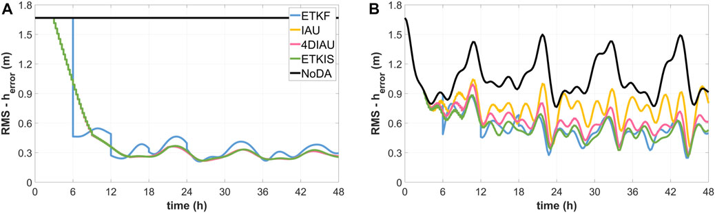
FIGURE 1. The time series of RMSE of the h variable in (A) the experiment with balanced initial conditions and (B) the experiment with imbalanced initial condition.

In Eq. 14, h is the depth deviation of the fluid from the average depth, H. u and v are the velocities in the x and y directions, respectively. H is set to 500 m and the Coriolis parameter, f = 10⁻⁴ rad/s. The model domain has rigid boundaries, and the range is 5,000 km with 101 grids in the abscissa with a grid spacing of 50 km. The model is integrated using the fourth-order Runge–Kutta scheme with a 15-min time step.

In the first OSSE, all experiments, including the nature run, are initialized from balanced conditions, in which the h variables are generated by Eq. 15a, and u and v variables are diagnosed by the geostrophic balance relationship (Eqs 15a,c). Experiments are conducted to verify whether the incremental update schemes can reduce the imbalance induced by covariance localization.

$\begin{array}{c}h=h_{amp}\times \cos \left(\frac{2\pi }{L}\left(x-x_{ps}\right)\right)\end{array},(\mathrm{15a})$

$\begin{array}{c}{\mathbf{u}}_{\text{g}}=-\frac{g}{f}\frac{\partial \mathbf{h}}{\partial y}=0\end{array},(\mathrm{15b})$

$\begin{array}{c}{\mathbf{v}}_{\text{g}}=\frac{g}{f}\frac{\partial \mathbf{h}}{\partial x}\end{array}.(\mathrm{15c})$

In Eq. 15a, the h_amp is the amplitude of depth deviation, x_ps is the phase shift, and L is the wavelength. The nature run has a stationary waveform (i.e., no propagation or oscillation), in which the values of h_amp, x_ps, and L are 10 m, −100, and 2,100 km, respectively. Following the setup used in the study by Greybush et al. [6], all DA experiments use five ensemble members with the same set of initial conditions generated by perturbing h_amp from 9 to 11, x_ps from −50 to 50 km, and L from 1,950 to 2,050 km. The wave in each member is in geostrophic balance and stationary until the adjustment from DA disrupts the balance.

The second OSSE is designed to investigate the ability of the incremental update schemes to correct the moving errors when the nature run carries propagating signals, and also how the moving signals in the corrections will be filtered by the schemes. The initial h of this nature run and ensemble for the DA experiments are taken from those of the first OSSE, but the initial u and v values are set to be zero. By destroying the balance, propagating waves are generated: a moving signal in the nature run and moving error originated from the initial condition in the experiments.

For both OSSEs, observations are generated every 24 steps (6-h) for h and v by adding random perturbations to each variable of the nature run, and the observation error is 10% of their amplitude (h = 1 m, v = 0.2932 m/s). Observations are available every five model grids (250 km). Under the ETKF framework, three incremental update schemes, ETKIS, IAU, and 4DIAU, are implemented. All experiments adopt the same assimilation parameter settings used in the study by Greybush et al. [6], including an R-localization scale of 500 km, the truncation distance of 2,000 km, and a multiplicative inflation of 5%. The localization scale is broader than the spacing of the observations (250 km). Therefore, the imbalances in model variables are not related to the arrangement of the observational network. Each experiment carried out four analysis cycles with an interval of 6 h and a 24-h forecast initialized from the final analysis. The root-mean-square error (RMSE) of h is used to evaluate the state accuracy, and the ageostrophic v wind is used to assess the amount of imbalance.

Results of the Experiment With Balanced Initial Conditions

When initializing the shallow-water system with a balanced condition, any projection on the ageostrophic component will result in imbalance and error (the nature run has zero ageostrophic wind). Figure 2 is the Hovmoller diagram of the ageostrophic v wind during the forecast-analysis cycles, showing the impact of the imbalance induced by performing DA. Significant ageostrophic wind is generated at the first analysis time (6-h) from the ETKF experiment (Figure 2A), and the imbalance propagates within the model domain and deflects due to the rigid boundaries. The analysis increments from later cycles do not eliminate this imbalance and even superpose more newly generated imbalance. In comparison to Figure 2A, there is very little discontinuity in IAU (Figure 2B). The reduced ageostrophic wind with much smoother structures in Figure 2B justifies IAU’s property of low-pass filtering. 4DIAU and ETKIS also have similar results as IAU (Figures 2C,D). However, the ETKIS experiment has slightly larger ageostrophic wind (Figures 2C vs. 2D). Such difference comes from the fact that, at each update step, ETKIS uses the incrementally smoothed ensemble model state to calculate the gradual correction (Eqs 5, 6), which contains the incompletely removed ageostrophic momentum from the previous gradual increment in the update window.

FIGURE 2

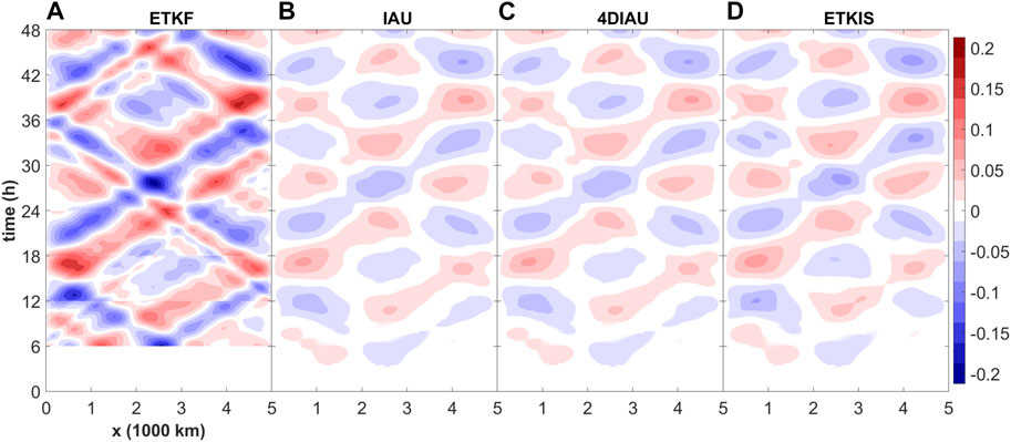
FIGURE 2. Evolution of the ageostrophic v wind in the shallow water experiments using different DA schemes: (A) ETKF, (B) IAU (C) 4DIAU and (D) ETKIS. Experiments are initialized from a balanced condition.

The h RMSEs from all experiments (Figure 1A) suggest that the performance of all incremental update schemes is comparable to that of the standard ETKF, which applies the full correction at once at the analysis time. In comparison with ETKIS and IAU/4DIAU schemes, the ETKF experiment exhibits larger oscillations in the RMSE due to the larger errors shown in the ageostrophic wind component.

Results of the Experiment With Imbalanced Initial Condition

In the second set of the experiments, we evaluate the performance of incremental update schemes in correcting the propagating errors with the condition that the nature carries fast-moving waves. To highlight the accumulated effect of the DA schemes in correcting the propagating errors, the cumulative correction is presented in Figure 3 and is defined as the difference between this no DA run and DA experiments.

FIGURE 3

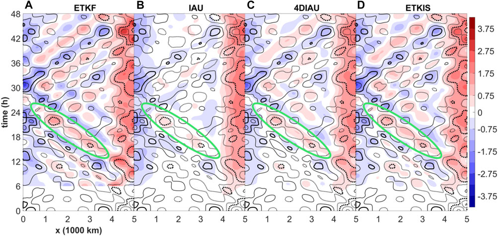
FIGURE 3. Temporal evolution of the h error (contour) and cumulative correction (shaded) in the shallow water experiments using different DA schemes: (A) ETKF, (B) IAU (C) 4DIAU, and (D) ETKIS. Experiments are initialized from a balanced condition. The cumulative correction is calculated as the difference between NoDA and DA experiments. Contour value ranges from −3.75 to −0.75 (dashed) and 0.75 to 3.75 m with 1-m interval; values of 1.75 and −1.75 are denoted with thick contours.

As the one-time update scheme, the pattern of the ETKF corrections (color shading in Figure 3) corresponds to those of the errors; however, the discontinuity at the analysis times is evident and leads to serious imbalance. Similar to what have been shown in Figure 2, IAU, 4DIAU, and ETKIS all work well in providing smooth corrections. However, the errors and signals are both propagating, and this increases the difficulty for the incremental update schemes to adapt the moving errors. Figure 3 shows that the cumulative corrections among these schemes are different in terms of filtering characteristics, and this affects their correction effect much. The high-frequency signals are strongly filtered by IAU, while they are more retained by 4DIAU and ETKIS. The difference in their filtering property comes from the fact that ETKIS and 4DIAU have flow-dependent gradual increment.

To illustrate the filtering mechanism of ETKIS and its difference from the IAU, Figure 4 shows the h increment at the end of the update window contributed from the gradual increment at each time step. Each increment is derived by the difference between the analysis mean of the first cycle (from 3rd to 9th h) using the full gradual increment and the one reconstructed without the gradual increment to be estimated. The earlier added gradual increments are integrated for more time steps in either scheme. However, IAU uses the same gradual increment at every time step in the update window, and the increments at the end of window will consequently have phase shifts (color lines in Figure 4A), which are caused by the displacement in time. Due to the phase shift, signals with high frequency tend to cancel out each other, and thus, IAU has a property of a low-pass filter. The averaged increment shows (black line in Figure 4A) that signals with a wavelength shorter than 1,500 km are strongly damped. In contrast, ETKIS uses flow-dependent gradual increments which adapt to the dynamical evolution, and thus tends to produce the same increments at the end of the update window. Therefore, the ETKIS gradual increments have the property of dynamical consistency. For this reason, the h increments of ETKIS at the end of the window have a similar pattern (Figure 4B) and retain much more small-scale corrections, which are proven to be valid, as shown in Figure 3D. Furthermore, ETKIS still smooths some signals which are not dynamically consistent. In Figure 4B, there is still phase shift which corresponds to the artificial waves induced by the covariance localization. Such artificial signals are independent to time, and consequently, its integration will have phase shift as the IAU increments. As a result, with such a mechanism, ETKIS can retain valid signals, since most of them are dynamically consistent, and still have a low-pass filtering for the dynamically inconsistent signals. With the corrections shown in Figure 3C, 4DIAU is expected to have flow-dependent gradual increment and has a similar selective filtering property. As will be discussed in Experiments with the Lorenz three-variable model section, the ETKIS will have better ability to retain dynamically consistent signals with the nonlinear dynamic system.

FIGURE 4

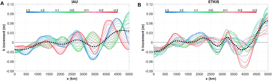
FIGURE 4. The h increment at t+3 (i.e., 9th hour) for gradual increment added during the update window from t−3 to t+3 (3rd hour to 9th hour) with (A) IAU and (B) ETKIS schemes. The black dot line is average of the h increments at t−3.

The selective filtering property is a key advantage of 4DIAU and ETKIS of computing the gradual increment with the time-evolving state and avoids the degeneracy with the IAU corrections (Figure 3B). For example, the moving correction, which started from 3,500 km at the 15th h–500 km at the 24th h (the green circles in Figure 3), was filtered seriously with IAU. In comparison, the corrections from 4DIAU and ETKIS retain most signals corresponding to error. Results suggest that ETKIS has a better capability in providing valid corrections than 4DIAU does, for instance, stronger corrections (Figure 3C vs. 3 days) and a lower RMSE than the ETKF in Figure 1B.

Results from two OSSEs show that ETKIS not only preserves the good correction from the ETKF scheme but also provides smooth update, which leads to a more balanced model state as the important purpose that incremental update schemes seek. More importantly, ETKIS shows a selective filtering property that only filters out high-frequency but dynamically inconsistent signals induced by the covariance localization in our experiment. This suggests that ETKIS could have the least sacrifice for the dilemma between improving the state balance and retaining effective correction.

Experiments With the Lorenz Three-Variable Model

Experiment Settings

This section presents how the ETKIS performs under the scenario of strong nonlinearity. OSSEs are conducted with the Lorenz three-variable model [31] to mimic such a scenario. The model state (x, y, and z) is governed by three equations (Eq. 16), where σ = 10, γ = 28, and β = 8/3 are model parameters chosen to generate the model nonlinear trajectory with two attractors (the butterfly pattern).

$\begin{array}{c}\frac{dx}{dt}=\sigma \left(y-x\right),\end{array}$

$\begin{array}{c}\frac{dy}{dt}=x\left(\gamma -z\right)-y,\end{array}(16)$

$\frac{dz}{dt}=xy-\beta z.$

The fourth-order Runge–Kutta scheme is used for time integration with a time step of 0.01. Hereafter, this model is referred to as the L63 model.

The nature run is a 60,000-step long simulation initialized from a spun-up model state, which is generated by integrating the model from a state of (8.0, 0.0, and 30.0) for 600 steps. Ten ensemble members are generated by adding Gaussian random values with a variance of nine to a chosen initial mean state, which is prepared by adding an error (−3, 3, −3) to the initial condition of the nature run. Observations are generated for all three variables by adding Gaussian random values with a variance of two to the nature state. The first set of observations is arranged at the 6th time step and available every 12 time steps afterward.

In the following, the results of the DA experiments are presented with the offline and online settings. The offline experiments aim to provide a clean illustration of the importance to have a time-varying gradual increment when strong nonlinearity takes place. The increment schemes use the same background ensemble at each assimilation window, and the impact of the incremental schemes is not cycled. For online experiments, the impact of the incremental schemes is cycled and accumulated. All online experiments are initialized from the same initial ensemble.

The performances of five schemes are compared in this section, including the ETKF, ETKIS, IAU, 4DIAU, and 4DIAU_EX. Each scheme is conducted with three different lengths of the assimilation window, including 12, 24, and 48 time steps, to investigate the sensitivity to the nonlinearity. With the observation setup, there will be one, two, and four sets of observations available for these three types of the assimilation window. The ETKF (and other update schemes) experiment uses the 4DETKF algorithm [21] in order to assimilate all observations within the assimilation window and produce an analysis trajectory. ETKIS, IAU, and 4DIAU perform the incremental update at every time step with an update window spanning the whole assimilation window. Unlike 4DIAU that only uses three analyses at the beginning, middle, and end of the update window, 4DIAU_EX uses full analysis trajectory from the ETKF to calculate the gradual increment and is expected to catch the nonlinear error evolution better than 4DIAU.

General Performance

The general performance of the analysis schemes is first evaluated according to the average RMSE of the analysis mean at the end of the assimilation window. Tables 1, 2 list the results categorized into four groups according to the perturbation growth rate of each DA cycle. The perturbation growth rate is defined for a period between the beginning of the DA cycle and analysis time. It is the averaged growth rate from 36 perturbation samples generated by combining the first two eigen modes of the tangent linear model of Eq. 16. The colored numbers in Tables 1, 2 indicate that the comparison to the ETKF RMSE is statistically significant. According to the perturbation growth rate, cycles are sorted into the groups of negative, low, mid, and high perturbation growth rates. The sample number is even among groups to avoid sampling errors for the following investigation.

TABLE 1

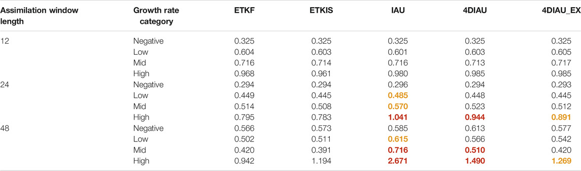
TABLE 1. Mean RMSE of the offline cycling experiments from different update algorithms. RMSE is calculated with the analysis mean at the end of the assimilation window. Numbers are highlighted if they are significantly higher (lower) than the ETKF RMSE. According to the t test, warm color indicates an RMSE significantly higher than the ETKF one. Darker and lighter color denote higher and medium confidence, corresponding to a level of 95 and 80%, respectively.

TABLE 2

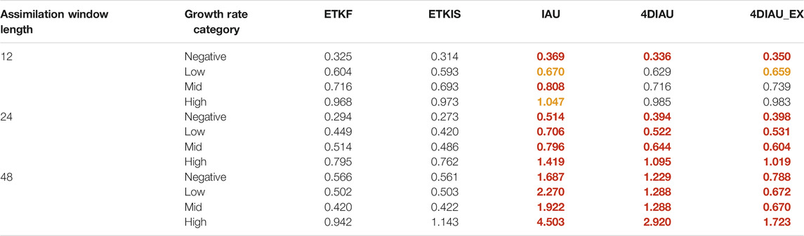
TABLE 2. RMSE of online cycling experiments. As Table 1, but for online cycling experiment.

Results from the offline experiments (Table 1) show that larger difference between the ETKF and incremental update schemes appears in the categories with higher perturbation growth rates and longer assimilation windows, that is, conditions of stronger nonlinearity. Compared with the ETKF, ETKIS keeps a comparable performance, while the remaining incremental update schemes show larger RMSEs. The smaller RMSE of 4DIAU_EX than that of 4DIAU confirms that 4DIAU_EX has better ability to catch the nonlinear error evolution.

Compared with Table 1, the result of the online cycling experiment (Table 2) shows the impact of each scheme accumulated through the forecast-analysis cycles. For IAU, 4DIAU, and 4DIAU_EX, their RMSEs increase in most of the categories and assimilation windows, especially for the ones with longer assimilation windows and a high perturbation growth rate. This indicates a negative feedback deteriorates the state accuracy when using IAU/4DIAU to update the state incrementally. By contrast, RMSE of ETKIS is smaller than those of the ETKF when the length of assimilation windows is shorter than 24 time steps.

Results from both the offline and online experiments indicate that ETKIS can achieve better accuracy than IAU and 4DIAU for conditions with strong nonlinearity. Focusing on an example with strong nonlinearity, we illustrate how ETKIS/4DIAU modifies the state accuracy in the next subsection.

An Example of the Time-Varying Gradual Increment

Focusing on an example with strong nonlinearity, we illustrate how ETKIS/4DIAU modifies the state accuracy in the next subsection. A case with a large perturbation growth rate is used to demonstrate how the flow-dependent gradual increment of ETKIS and 4DIAU is different. The example is taken from the update process during the 316th cycle from the offline experiments with a 24-time step assimilation window in which the observations are available at 6th and 18th time steps. It should be noted that the innovation at the 18th time step is large (−3.162 for the z variable) because the ensemble mean has large error due the strong nonlinearity. Given the same background ensemble, the derived weights are the same in all schemes with Eqs 3, 4, but the way to use these weights to derive increments varies in all schemes. Thus, it is not anticipated to keep the same effect on constraining the ensemble spread after translating the one-time correction into time-varying increments.

The ensemble states of this cycle start at a condition close to bifurcation, at which the model evolution is very sensitive to the initial condition. Figure 5 shows the initial condition and evolution of the same five selected ensemble states from different schemes during this cycle. The initial condition of these ensemble members located in both regimes and the ensemble members disperse quickly during the forecast, leading to a large ensemble spread. The error evolution is also highly nonlinear with a fast growth rate (black line in Figures 6A–D).

FIGURE 5

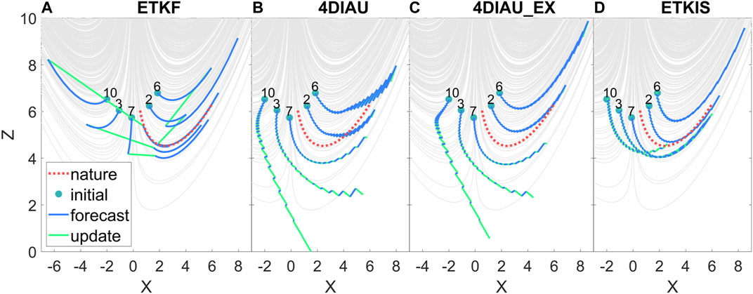
FIGURE 5. The trajectories of ensemble forecast (blue) and nature (red) during the 316th DA cycle with the L63 model with different DA schemes: (A) ETKF, (B) 4DIAU (C) 4DIAU_EX and (D) ETKIS. The green dot is the initial condition of the ensemble member and the green line is the adjustment of the DA scheme from the offline experiment. The number corresponds to the ensemble member number. The gray line is a trajectory from long-term free integration to exhibit the nonlinear behavior of the L63 model. Only five ensemble members are selected for clear illustration.

FIGURE 6

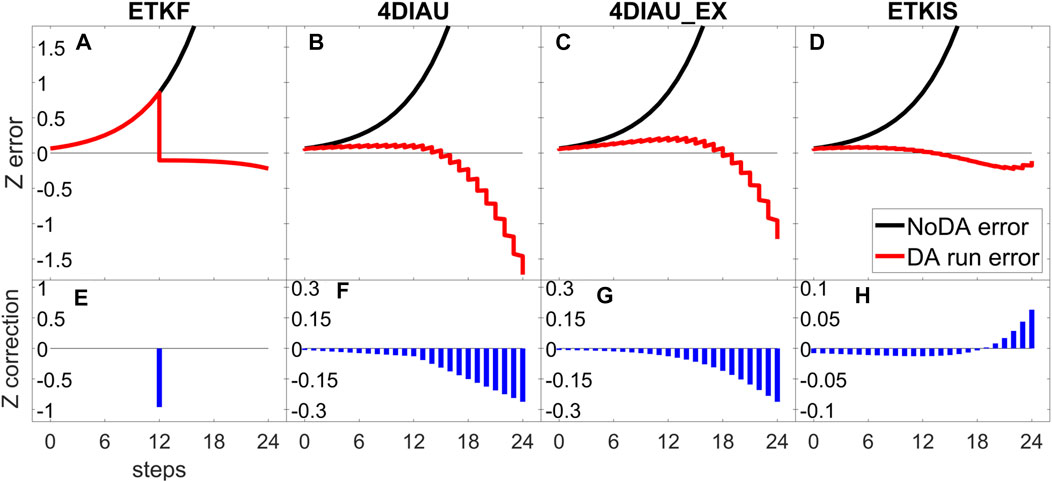
FIGURE 6. The error and increment during the 316th DA cycle in the offline cycling experiment for the ETKF, ETKIS, 4DIAU, and 4DIAU_EX. The upper panel (A–D) shows the error evolution of the z variable: the black line indicates how the error grows without correction, and the red line indicates how the error evolves after applying the analysis increment. The lower panel shows the (E) analysis increment and (F–H) gradual increment of the z variable.

Taking the trajectory of the ETKF as an example (Figure 5A), most ensemble members evolve faster than nature, and the error of the z-variable background mean grows quickly (black line in Figure 6A). With the large ensemble spread and innovation, the ETKF makes strong corrections at the analysis time (Figure 6E), which pull the over-evolving members back and result in a strong discontinuity, especially those members in the wrong regime (e.g., a correction of −2.846 for member 10). With the analysis trajectory from the ETKF, the gradual increments derived by the 4DIAU and 4DIAU_EX (Figures 6F,G) are well proportional to the evolution of the background error (black line in Figure 6B). Their gradual increments during the second half of the update window have large magnitude corresponding to the great z error due to the fast-growing ensemble spread during the update window and partially the large innovation at the 18th time step. The 4DIAU incremental update process successfully corrects the ensemble during the first half of the update window (red line in Figure 6B), pulling the ensemble members toward the correct regime (Figure 5B). Thus, the ensemble evolution has been improved, and the need for a negative correction in z becomes less. Therefore, the large gradual increments at later time steps become unsuitable to the incrementally updated ensemble. They do not provide useful corrections and fail to shrink the ensemble spread. The gradual increments with large and negative values eventually overcorrect the z value and lead to an analysis worse than that of the ETKF (Figures 5B vs. 5A). As shown in Figure 5B, the z variable of the 3rd and 10th members are overcorrected to a value much smaller than the nature, and their state evolution does not follow the model behavior, that is, a very imbalanced condition. In other words, the incremental corrections at later steps, derived for the original background trajectories, cannot correspond to the errors that existed in the modified ensemble and thus degrade the accuracy of analysis and the following prediction. For the same reason, even when using gradual increment derived by a full analysis trajectory, the 4DIAU_EX is still not able to achieve better performance. This example also indicates that 4DIAU has difficulty in constraining the ensemble spread under the condition of a fast perturbation growth rate.

By contrast, the ensemble in ETKIS can smoothly evolve into the correct regime with the gradual increment, and the ensemble spread in ETKIS is more constrained than in 4DIAU. The amount of gradual increment in ETKIS is much smaller than that in either the ETKF or 4DIAU, and its sign alters during the incremental update process (at the 19th step on Figure 6D). During ETKIS’s incremental update process, the evolution of the ensemble forecast is modified and the weights are applied to the updated ensemble space. The incremental correction adapts the evolution of the ensemble, and the overcorrection shown in the 4DIAU z variable is avoided in ETKIS. This example illustrates that ETKIS has the advantage of allowing the incremental correction having a temporal variation corresponding to the error evolution during the update steps. Such property is particularly beneficial during strong nonlinearity.

Summary

This study proposes a new incremental update scheme, ETKIS, based on the framework with the ETKF algorithm. In addition to the optimal purpose of incremental update schemes that reduce the imbalance from DA correction, ETKIS mitigates the degradation caused by the nonlinear evolution during the update window. The traditional incremental update schemes (IAU and 4DIAU) use the background trajectory to calculate the analysis increment and update the model state with gradual increment. Unlike applying temporal interpolation to the analysis increment in 4DIAU, ETKIS constructs time-varying increments by distributing the ETKF weight coefficients to each update step and applying them to the evolving ensemble state. Two numerical models, the shallow-water model and the L63 model, with simple dynamics are used to verify the ability of ETKIS to mitigate imbalance and highlight the challenge in the application of the incremental update schemes under nonlinear dynamics.

When the shallow-water model is initialized by a balanced state, the one-time analysis correction made by the ETKF results in serious imbalance in the ageostrophic wind due to the use of covariance localization. Result confirms that ETKIS has the ability to mitigate the imbalance and its performance is comparable to that of IAU and 4DIAU. With another scenario that propagating signals exist in both nature and initial errors, the flow-dependent incremental correction from ETKIS helps to capture the propagating error better than that from 4DIAU, while IAU has the worst performance, and its correction is overly smoothed out. Conclusively, ETKIS has the advantage of selective filtering which damps high-frequency correction like IAU does, but retains signals with dynamical consistency. The incremental updates from ETKIS can be regarded as a mechanism like constructive interference.

Results from the experiments with the L63 model show that ETKIS provides a more accurate model state than 4DIAU at the end of the assimilation window, in particular for the conditions with strong nonlinearity (conditions with long assimilation window and a high perturbation growth rate).

An example with the initial model state close to bifurcation illustrates that the fast-growing (and large) ensemble spread leads to large analysis increment at later analysis time in 4DIAU’s update window. After applying temporal interpolation to the analysis increments at different update times, large gradual increments appear in the latter half of the update window. However, once the model state at the early steps in the assimilation window has been corrected, there is no need for such large correction at later steps and the state accuracy at the end of the assimilation window is degraded due to overcorrection. Such an ensemble cannot well present the error structure and could degrade the DA performance in the following cycle. For the same reason, 4DIAU is less effective to compress the ensemble spread and results in an overestimated ensemble spread. Thus, the detrimental impact is accumulated in the online experiments. By contrast, ETKIS applies the precomputed weight to the ensemble evolved from the previous time step of incremental update to calculate the correction. This helps the ETKIS increment capture more current error and reduce the forecast error effectively. Also, the constrained spread allows the following increment to have a modest amplitude. For this simple nonlinear model, ETKIS can catch the nonlinearly evolving error during increment update. The correction from ETKIS can give considerations to provide a smooth and moderate update process and provide better accuracy than 4DIAU. In conclusion, ETKIS can be regarded as a more robust choice to gain the benefit from the incremental process and maintain the effective correction from the ETKF under nonlinear dynamics.

Although the incremental update schemes involving interpolating the analysis increments can mitigate the model shock and gently bring in the impact of assimilating observations, this study points out that a potential issue could appear when dealing with conditions with strong nonlinearity, such as the development of severe weather systems like tropical cyclones (TC). Currently, ETKIS has been implemented in a regional EnKF system to investigate its impact on mitigating the spin-up issue when the model TC structure is adjusted in responding to the analysis corrections from assimilating inner-core dropsonde data [32]. We also note that ETKIS could be incorporated with other EnKF frameworks, such as the iterative EnKF [33], in which a cost function is constructed with the weight coefficient as the control variable, and the minimization is solved by the iterative method.

Data Availability Statement

The raw data supporting the conclusion of this article will be made available by the authors, without undue reservation.

Author Contributions

Z-HL was in charge of the implementation and evaluation of the algorithm. S-CY proposed the original method, advised this work, and provided scientific discussions. Z-HL and S-CY prepared the manuscript jointly. EK provided comments and suggestions for improving this manuscript.

Funding

Z-HL and S-CY were supported by the Ministry of Science and Technology in Taiwan (MOST-109-2111-M-008-014 and MOST-110-2923-M-008-003-MY2).

Conflict of Interest

The authors declare that the research was conducted in the absence of any commercial or financial relationships that could be construed as a potential conflict of interest.

References

1. Kalnay, E. Atmospheric Modeling, Data Assimilation and Predictability. Cambridge University Press (2002). doi:10.1017/CBO9780511802270

CrossRef Full Text

2. Evensen, G. Sequential Data Assimilation with a Nonlinear Quasi-Geostrophic Model Using Monte Carlo Methods to Forecast Error Statistics. J Geophys Res (1994) 99:10143–62. doi:10.1029/94JC00572

CrossRef Full Text | Google Scholar

3. Burgers, G, van Leeuwen, PJ, and Evensen, G. Analysis Scheme in the Ensemble Kalman Filter. Mon Wea Rev (1998) 126:1719–24. doi:10.1175/1520-0493(1998)126<1719:ASITEK>2.0.CO;2

CrossRef Full Text | Google Scholar

4. Pu, Z, Zhang, S, Tong, M, and Tallapragada, V. Influence of the Self-Consistent Regional Ensemble Background Error Covariance on Hurricane Inner-Core Data Assimilation with the GSI-Based Hybrid System for HWRF J Atmos Sci (2016) 73:4911–25. doi:10.1175/JAS-D-16-0017.1

CrossRef Full Text | Google Scholar

5. Lorenc, AC. The Potential of the Ensemble Kalman Filter for NWP-A Comparison with 4D-Var. Q.J.R Meteorol Soc (2003) 129:3183–203. doi:10.1256/qj.02.132

CrossRef Full Text | Google Scholar

6. Greybush, SJ, Kalnay, E, Miyoshi, T, Ide, K, and Hunt, BR. Balance and Ensemble Kalman Filter Localization Techniques. Mon Wea Rev (2011) 139:511–22. doi:10.1175/2010MWR3328.1

CrossRef Full Text | Google Scholar

7. Gaspari, G, and Cohn, SE. Construction of Correlation Functions in Two and Three Dimensions. Q.J R Met. Soc. (1999) 125:723–57. doi:10.1002/qj.49712555417

CrossRef Full Text | Google Scholar

8. Miyoshi, T, Kondo, K, and Imamura, T. The 10,240-member Ensemble Kalman Filtering with an Intermediate AGCM. Geophys Res Lett (2014) 41:5264–71. doi:10.1002/2014GL060863

CrossRef Full Text | Google Scholar

9. Lange, H, and Craig, GC. The Impact of Data Assimilation Length Scales on Analysis and Prediction of Convective Storms. Mon Wea Rev (2014) 142:3781–808. doi:10.1175/MWR-D-13-00304.1

CrossRef Full Text | Google Scholar

10. Bloom, SC, Takacs, LL, Da Silva, AM, and Ledvina, D. Data Assimilation Using Incremental Analysis Updates. Mon Wea Rev (1996) 124:1256–71. doi:10.1175/1520-0493(1996)124<1256:DAUIAU>2.0.CO;2

CrossRef Full Text | Google Scholar

11. Lea, DJ, Mirouze, I, Martin, MJ, King, RR, Hines, A, Walters, D, et al. Assessing a New Coupled Data Assimilation System Based on the Met Office Coupled Atmosphere-Land-Ocean-Sea Ice Model. Mon Wea Rev (2015) 143:4678–94. doi:10.1175/MWR-D-15-0174.1

CrossRef Full Text | Google Scholar

12. Rienecker, M. M., Suarez, M. J., Todling, R., Bacmeister, J., Takacs, L., Liu, H.-C., et al. (2008) The GEOS-5 Data Assimilation System - Documentation of Versions 5.0.1, 5.1.0, and 5.2.0. NASA GSFC Technical Report Series on Global Modeling and Data Assimilation, 27, link: https://gmao.gsfc.nasa.gov/pubs/docs/Rienecker369.pdf

Google Scholar

13. Lee, M-S, Kuo, Y-H, Barker, DM, and Lim, E. Incremental Analysis Updates Initialization Technique Applied to 10-km MM5 and MM5 3DVAR. Mon Wea Rev (2006) 134(5):1389–404. doi:10.1175/MWR3129.1

CrossRef Full Text | Google Scholar

14. Huang, B, Kinter, JL, and Schopf, PS. Ocean Data Assimilation Using Intermittent Analyses and Continuous Model Error Correction. Adv Atmos Sci (2002) 19:965–92. doi:10.1007/s00376-002-0059-z

CrossRef Full Text | Google Scholar

15. Carton, JA, Chepurin, G, Cao, X, and Giese, B. A Simple Ocean Data Assimilation Analysis of the Global Upper Ocean 1950–95. Part I: Methodology. J Phys Oceanogr (2000) 30:294–309. doi:10.1175/1520-0485(2000)030<0294:ASODAA>2.0.CO;2

CrossRef Full Text | Google Scholar

16. Ourmières, Y, Brankart, J-M, Berline, L, Brasseur, P, and Verron, J. Incremental Analysis Update Implementation into a Sequential Ocean Data Assimilation System. J Atmos Oceanic Technol (2006) 23:1729–44. doi:10.1175/JTECH1947.1

CrossRef Full Text | Google Scholar

17. Yan, Y, Barth, A, and Beckers, JM. Comparison of Different Assimilation Schemes in a Sequential Kalman Filter Assimilation System. Ocean Model (2014) 73:123–37. doi:10.1016/j.ocemod.2013.11.002

CrossRef Full Text | Google Scholar

18. Lorenc, AC, Bowler, NE, Clayton, AM, Pring, SR, and Fairbairn, D. Comparison of hybrid-4DEnVar and hybrid-4DVar Data Assimilation Methods for Global NWP. Mon Wea Rev (2015) 143:212–29. doi:10.1175/MWR-D-14-00195.1

CrossRef Full Text | Google Scholar

19. Buehner, M, McTaggart-Cowan, R, Beaulne, A, Charette, C, Garand, L, Heilliette, S, et al. Implementation of Deterministic Weather Forecasting Systems Based on Ensemble-Variational Data Assimilation at Environment Canada. Part I: The Global System. Mon Wea Rev (2015) 143:2532–59. doi:10.1175/MWR-D-14-00354.1

CrossRef Full Text | Google Scholar

20. Lei, L, and Whitaker, JS. A Four-Dimensional Incremental Analysis Update for the Ensemble Kalman Filter. Mon Wea Rev (2016) 144:2605–21. doi:10.1175/MWR-D-15-0246.1

CrossRef Full Text | Google Scholar

21. Hunt, BR, Kostelich, EJ, and Szunyogh, I. Efficient Data Assimilation for Spatiotemporal Chaos: A Local Ensemble Transform Kalman Filter. Physica D: Nonlinear Phenomena (2007) 230:112–26. doi:10.1016/j.physd.2006.11.008

CrossRef Full Text | Google Scholar

22. Kalnay, E, Li, H, Miyoshi, T, Yang, S-C, and Ballabrera-Poy, J. Response to the Discussion on "4-D-Var or EnKF?" by Nils Gustafsson. Tellus A: Dynamic Meteorol Oceanogr (2007) 59:778–80. doi:10.1111/j.1600-0870.2007.00263.x

CrossRef Full Text | Google Scholar

23. Sakov, P, Oliver, DS, and Bertino, L. An Iterative EnKF for Strongly Nonlinear Systems. Mon Wea Rev (2012) 140:1988–2004. doi:10.1175/MWR-D-11-00176.1

CrossRef Full Text | Google Scholar

24. Kalnay, E, and Yang, S-C. Accelerating the Spin-Up of Ensemble Kalman Filtering. Q.J.R Meteorol Soc (2010) 136:1644–51. doi:10.1002/qj.652

CrossRef Full Text | Google Scholar

25. Yang, S-C, Kalnay, E, Hunt, B, and E. Bowler, N. Weight Interpolation for Efficient Data Assimilation with the Local Ensemble Transform Kalman Filter. Q.J.R Meteorol Soc (2009) 135:251–62. doi:10.1002/qj.353

CrossRef Full Text | Google Scholar

26. Bishop, CH, Etherton, BJ, and Majumdar, SJ. Adaptive Sampling with the Ensemble Transform Kalman Filter. Part I: Theoretical Aspects. Mon Wea Rev (2001) 129:420–36. doi:10.1175/1520-0493(2001)129<0420:ASWTET>2.0.CO;2

CrossRef Full Text | Google Scholar

27. Wang, X, and Bishop, CH. A Comparison of Breeding and Ensemble Transform Kalman Filter Ensemble Forecast Schemes. J Atmos Sci (2003) 60:1140–58. doi:10.1175/1520-0469(2003)060<1140:ACOBAE>2.0.CO;2

CrossRef Full Text | Google Scholar

28. Bergemann, K, and Reich, S. A Mollified Ensemble Kalman Filter. Q.J.R Meteorol Soc (2010) 136:1636–43. doi:10.1002/qj.672

CrossRef Full Text | Google Scholar

29. Gottwald, GA. Controlling Balance in an Ensemble Kalman Filter. Nonlin Process. Geophys (2014) 21:417–26. doi:10.5194/npg-21-417-2014

CrossRef Full Text | Google Scholar

30. Gauthier, P, and Thépaut, J-N. Impact of the Digital Filter as a Weak Constraint in the Preoperational 4DVAR Assimilation System of Météo-France. Mon Wea Rev (2001) 129:2089–102. doi:10.1175/1520-0493(2001)129<2089:iotdfa>2.0.co;2

CrossRef Full Text | Google Scholar

31. Lorenz, EN. Deterministic Nonperiodic Flow. J Atmos Sci (1963) 20:130–41. doi:10.1175/1520-0469(1963)020<0130:DNF>2.0.CO;2

CrossRef Full Text | Google Scholar

32. Lin, Z-H, Yang, S-C, and Lin, K-J. Ensemble Transform Kalman Incremental Smoother and its Potential on Severe Weather Prediction. In: AOGS 16th Annual Meeting. Singapore:Asia Oceanic GeoScience Society (2019). p. AS12–A02s.

Google Scholar

33. Bocquet, M, and Sakov, P. Combining Inflation-free and Iterative Ensemble Kalman Filters for Strongly Nonlinear Systems. Nonlin Process. Geophys (2012) 19:383–99. doi:10.5194/npg-19-383-2012

CrossRef Full Text | Google Scholar

34. Nino-Ruiz, E., Sandu, A., and Deng, X. (2018). An Ensemble Kalman Filter Implementation Based on Modified Cholesky Decomposition for Inverse Covariance Matrix Estimation. SIAM J. Sci. Comput. 40 (2), A867–A886. doi:10.1137/16M1097031