Oscillatory Biomedical Signals: Frontiers in Mathematical Models and Statistical Analysis

1 Introduction

The 2017 Nobel Prize in Physiology or Medicine was awarded to Jeffrey Hall and Michael Rosbash of Brandeis University, and Michael Young of Rockefeller University, “for their discoveries of molecular mechanisms controlling the circadian rhythm.” In 1984, they succeeded in isolating the “period gene” (i.e., the gene that controls the circadian rhythm). Hall and Rosbash then went on to “discover PER, the protein encoded by period, accumulated during the night and degraded during the day.” In 1994, Young answered a “tantalizing puzzle” concerning how PER produced in the cytoplasm could reach the cell nucleus where genetic material is located. He discovered a second gene timeless, encoding the TIM protein so that TIM bound to PER can enter the cell nucleus to block the period gene activity. “Such a regulatory feedback mechanism explained how this oscillation of cellular protein levels emerged, but questions lingered,” such as what controlled the frequency of the oscillations. Young identified another gene doubletime encoding the DBT protein that delayed the accumulation of the PER protein. The three laureates identified additional proteins required for the activation of the period gene, as well as for the mechanisms by which light can synchronize the circadian clock.

One of us (Muotri) was PI of a project on “spontaneous network formation” displaying “periodic and regular oscillatory events that were dependent on glutamatergic and GABAergic signaling” during early the brain maturations, for which structural and transcriptional changes “follow fixed developmental programs defined by genetics,” see [1] who also found that “the oscillatory activity transitioned to more spatiotemporally irregular patterns which synchronous network activity resembled features similar to those observed in preterm human EEG.” This project is similar in spirit to the exemplary work of Hall, Rosbash, and Young but the “experimental inaccessibility” of the human brain during the early stages of life pushes mathematical modeling and statistical analysis of the oscillatory signals and events to new frontiers that we present in the next section. We describe in the next paragraph the underlying biomedical background of this project.

One of the major recent realizations, especially in the neurosciences, is that while we can obtain important information from animal studies, there are major differences between humans and animals. This is manifested in many ways, especially in those major clinical trials based on animal findings that did not pan out. Therefore, if we intend to study pathogenesis of disease, treat them, prevent them, or cure diseases across the age spectrum, we need to refocus our scientific approaches and strategies in order to be more efficient and effective. Since embryonic stem cells are often problematic to obtain for ethical reasons, the discovery of being able to re-program somatic cells from humans into induced pluro-potential stem cells (iPSCs, taking these somatic cells back into their “history”) and differentiate them into different relatively mature cell types have opened a major avenue for the scientific community, resulting in the 2012 Nobel Prize in Physiology or Medicine to John Gurdon of Cambridge and Shinya Yamanaka of Kyoto. If these iPSCs are exposed to the right growth factors, they would assemble into the early human brain (brain organoids) by an amazing process of self-organizing the 3-dimensional cellular elements that recapitulate the network, cellular, and membrane properties of neurons and the glia. Many types of organoids such as the kidney, the intestine, the liver, and the lung organoids have been recently developed. These organoids have been particularly useful for studying either normal early human biology or developmental disorders as in neurodevelopmental diseases.

2 Methods

The statistical methods used by Trujillo et al. (2019, pp. 16–19) in their analysis of data on oscillatory signals and events consist of 1) multi-electrode array (MEA) recording and custom analysis, 2) network event analysis that involves detecting spikes (when at least 80% of the maximum spiking values) over the length of the recording when reached at least 1 s away from any other network event, 3) oscillatory spectral power analysis, in which “oscillatory power” is defined as “peaks in the PSD (power spectral density estimated by Peter D. Welch’s method) above the aperiodic $1/f$ power law decay,” and 4) resampled Pearson’s correlation coefficient between neonatal age and each of 12 EEG features. Because of “the inability to interrogate the electrophysiology of intact human brains” and the emergence of induced pluripotent stem cells (iPSCs) and organoids as “a scaled-down and three-dimensional model of the human brain, mimicking various developmental features at cellular and molecular levels,” [1, pp. 4, 7–9, 18] used oscillatory dynamics of LFP (local field potential) and other mesoscopic brain signals, which manifest “a phenomenon known as cross-frequency phase-amplitude coupling (PAC) wherein the high-frequency content of LFP is entrained to the phase of slow oscillations.” Noting that “the pattern of alternating periods of quiescence and network-synchronized events resembles electrophysiological signatures in preterm human EEG,” [1] analyzed “a publicly available dataset of 101 serial EEG recordings from 39 preterm infants ranging from 24 to 38 weeks post-menstrual age,” containing 23 precomputed features (including spectral power in canonical oscillatory bands, duration, and timing of “spontaneous activity transients” or SATs) for each EEG record. To compare the features between cortical organoids and preterm infants, [1] trained a regularized regression model (ElasticNet) with cross-validation for hyparameter selection based on the preterm infants’ EEG recordings and applied the model to the organoid dataset to “obtain the predicted developmental time.” The results were mixed and [1] concluded that “given the potential roles of synchronized and oscillatory network dynamics in coordinating information flow between developed brain regions, these results highlight the potential for cortical organoids to advance our understanding of functional physiology” and to model “cellular interactions and neural circuit dysfunctions related to neurodevelopmental and neuropsychiatric pathologies” that “affect millions of people but otherwise lack an existing animal model.” These statistical methods are “custom” (or traditional) methods, as acknowledged by [1]. We describe innovative and powerful methods in the next two subsections, first for time–frequency analysis of oscillatory biomedical signals with time-varying features and then a new hidden Markov model (HMM) which incorporates the key features of the cortical organoid model and provides uncertainty quantification for empirical Bayes inference based on the model and observed data.

2.1 Time–Frequency Analysis of Signals With Multiple Oscillatory Components

The first author (Wu) has been working on time–frequency analysis (TFA) and its applications to high-frequency biomedical signals in the last ten years. Examples include electrocardiography, electroencephalogram, local field potential, photoplethysmogram (PPG), actinogram, peripheral venous pressure (PVP), arterial blood pressure, phonocardiogram, and airflow respiratory signal, to name several. Usually, these signals are composed of multiple components, each of which reflects the dynamics of a physiological system. The analysis is challenged by the physiological variability that appears in the form of time-varying frequency and amplitude or even time-varying oscillatory pattern that is referred to as the “wave-shape function.” Furthermore, depending on the signal, the “waxing and waning” effect is sometimes inevitable for its components; see [2, Figure 1] for an illustration. Take the widely applied PPG signal as an example, for which [3] has given an introduction to photoplethysmogram (PPG) and its applications “beyond the calculation of arterial oxygen saturation and heart rate.” In addition to the well-known cardiac component reflecting hemodynamic information, PPG may contain the respiratory dynamics as another component. The frequency of the cardiac component (respiratory component, respectively) is impacted by the heart rate variability (breathing rate variability, respectively). Cicone and [4] provide an algorithm to “extract both heart and respiratory rates” from the PPG signal and thereby to analyze their interactions. Such information can be used in conjunction with other biomedical signals reflecting hemodynamics. In particular, PVP is ubiquitous in the hospital environment and a rich source of hemodynamic information [5]. But, it typically has a low signal-to-noise ratio (SNR), and its oscillatory pattern is sensitive to the physiological status, making it much less used in comparison with PPG. Wu et al. [6] have developed new signal processing tools to facilitate its use.

Combining time–frequency analysis (TFA) with statistical analysis, the lack of which in the previous work “presents an opportunity for much future research,” is illustrated in Figure 2 (applied to PPG, fetal ECG, and fetal heart rate variability) of Wu [2] who describes several recent advances in TFA for high-frequency biomedical signals. There are several challenges common to different biomedical signal processing problems. The first is how to estimate the dynamics (e.g., how to quantify the time-varying frequency, amplitude, or wave-shapes) of the signal. The second is to assess signal quality and determine artifacts, distinguishing between physiological and nonphysiological ones. The third is to identify oscillatory components and the fourth is to decompose the signal into constituent components. To address these challenges, several TFA tools have been proposed. In addition to the traditional linear-type time–frequency analysis tools like short-time Fourier transform (STFT), continuous wavelet transform (CWT), and bilinear time-frequency analysis tools [7], several nonlinear-type tools have been developed and applied, including the reassignment method, empirical mode decomposition (EMD), Blaschke decomposition (BKD), adaptive locally iterative filtering (ALIF), sparse time-frequency representation (STFR), synchrosqueezing transform (SST), scattering transform (ST), concentration of frequency and time (ConcFT), de-shape and dynamic diffusion maps [8–14]. The statistical properties of these methods have been relatively unexplored and we are currently investigating them; new methods to handle emerging scientific problems might be developed on the way.

2.2 Efficient Particle Filters for Joint State and Parameter Estimation in HMM

During the past three years, the second author (Lai) has been developing a new Markov Chain Monte Carlo (MCMC) procedure called “MCMC with sequential substitutions” (MCMC-SS) for joint state and parameter estimation in hidden Markov models. The basic idea is to approximate an intractable distribution of interest (or target distribution) by the empirical distribution of N representative atoms, chosen sequentially by an MCMC procedure, so that the empirical distribution approximates the target distribution after a large number of iterations as explained below.

Lai’s work in this area began with the landmark paper of Gordon, Salmond and Smith [15] on the development of sequential Monte Carlo (SMC), also called particle filters, for the estimation of latent states in a hidden Markov model (HMM). Liu’s monograph [16] contains a collection of techniques that have been developed since then, with examples of applications in computational biology and engineering, and Chan and Lai [17] provide a general theory of particle filters. Let $=\{X_t,t\mathrm{⩾}1\}$ be a Markov chain and let $Y_1,Y_2,\dots$ be conditionally independent given, such that $X_t\sim p_t(\cdot |X_{t-1}),Y_t\sim g_t(\cdot |X_t)$ in which $p_t$ and $g_t$ are density functions with respect to measures ${\nu }_X$ and ${\nu }_Y$. The density function $p_T$ of $X_{0:T}=\left(X_0,\dots ,X_T\right)$ conditional on $Y_{1:T}=\left(Y_1,\dots ,Y_T\right)$ is given by

$p_T\left(x_{0:T}|Y_{1:T}\right)\propto {\displaystyle \prod }_{t=1}^T\left[p_t\left(x_t|x_{t-1}\right)g_t\left(Y_t|x_t\right)\right].$

This conditional distribution is often difficult to sample from and the normalizing constant is also difficult to compute for high-dimensional or complicated state spaces, and particle filters use sequential Monte Carlo that involves importance sampling and resampling to circumvent this difficulty. The particle filter computes $\mathcal{E}\left[\psi \left(X_{0:T}\right)\right|Y_1,\dots ,Y_T]$ by the recursive Monte Carlo scheme summarized in Algorithm 1. Let $X_{0:t-1}^m$ denote the sample path of the mth particle (trajectory), $1\mathrm{⩽}m\mathrm{⩽}M$. The scheme uses importance sampling from a proposal density $q_t$ to circumvent this difficulty and updates not only the particles $X_{0:t-1}^m$ but also the associated weights $w_{t-1}^m$ and ancestor $A_{t-1}^m$ of $X_{0:t}^m$. It is initialized with $A_0^m=m$ and $w_0^m=1$. The SMC estimate of ${\psi }_T:=\mathcal{E}\left[\psi \left(X_{0:T}\right)\right|Y_{1:T}]$ is given by:

${\tilde{\psi }}_T=\left({\displaystyle \sum }_{m=1}^M{w}_T^m\psi \left(X_{0:T}^m\right)\right)/\left({\displaystyle \sum }_{m=1}^M{w}_T^m\right).$

By using martingale theory, Chan and Lai [17] provide a comprehensive theory of the SMC estimate ${\tilde{\psi }}_T$, which includes asymptotic normality and consistent standard error estimation as follows:

Theorem 1. Under certain Integrability Conditions,

$\sqrt{M}\left({\tilde{\psi }}_t-{\psi }_T\right)\Rightarrow N\left(0,{\sigma }^2\right).$

Moreover, letting ${\overline{w}}_t=M^{-1}{{{\displaystyle \sum }}^{\text{}}}_{i=1}^M{w}_t^i$, ${\sigma }^2$ can be consistently estimated by the following equation:

${\tilde{\sigma }}^2=\frac{1}{M}{\displaystyle \sum }_{m=1}^M{\left({\displaystyle \sum }_{i:A_{T-1}^i=m}\frac{w_T^i}{{\overline{w}}_T}[\psi \left(X_{0:T}^i\right)-{\tilde{\psi }}_T]\right)}^2.$

ALGORITHM 1

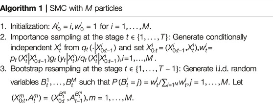
Algorithm 1. SMC with M particles

Chan and Lai [17, Lemmas 1 and 4] use the following representation of ${\tilde{\psi }}_T-{\psi }_T$ to derive Theorem 1. Let $w_t\left(x_{0:t}\right)=p_t\left(x_t|x_{t-1}\right)g_t\left(Y_t|x_t\right)/q_t\left(x_t|x_{0:t-1}\right)$, in which that $Y_t$ can be treated as constants since the particle filter is the conditional distribution of $X_{0:t}$ given the observations $Y_1,\dots ,Y_T$. Let $H_t^m=\left({\overline{w}}_1,\dots ,{\overline{w}}_t\right)/{{{\displaystyle \prod }}^{\text{}}}_{j1}^t{w}_j^m,{\eta }_t={\mathcal{E}}_q\left[{{{\displaystyle \prod }}^{\text{}}}_{i=1}^t{w}_i\left(X_{0:t}\right)\right]$, where ${\mathcal{E}}_q$ denotes expectation under which $X_t|X_{0:t-1}$ has the conditional density function $q_t(\cdot |X_{0:t-1})$ for $1\mathrm{⩽}t\mathrm{⩽}T$. Letting ${\text{Ψ}}_0={\psi }_T$ and ${\text{Ψ}}_t\left(X_{0:t}\right)={\mathcal{E}}_q\left\{\psi \left(X_{0:T}\right){{{\displaystyle \prod }}^{\text{}}}_{i=1}^T{w}_i\left(X_{0:i}\right)|X_{0:t}\right\}$ for $1\mathrm{⩽}t\mathrm{⩽}T$, define

$\begin{array}{l}{\mathit{ϵ}}_{2t-1}^m={\displaystyle \sum }_{i:A_{t-1}^m=m}\left\{\psi \left(X_{0:t}^i\right)-{\text{Ψ}}_{t-1}\left(x_{0:t-1}^i\right)\right\}{H}_{t-1}^i,\\ {\mathit{ϵ}}_{2t}^m={\displaystyle \sum }_{i:A_{t-1}^m=m}\left({\#}_t^m-m{W}_t^i\right)\left\{{\text{Ψ}}_t\left(X_{0:t}^i\right)H_t^{B_t^i}-{\text{Ψ}}_0\right\},\end{array}$

in which $W_t^i=w_t^i/{{{\displaystyle \sum }}^{\text{}}}_{j=1}^M{w}_t^j$, ${\#}_t^i$ is the number of copies of $X_{0:t}^i$ generated by bootstrap resampling from $\left\{X_{0:t}^1,\dots ,X_{0:t}^M\right\}$ in Algorithm 1 (where the $B_t^i$ is also defined). Then $\left({\#}_t^1,\dots ,{\#}_t^M\right)\sim \text{Multinomial}\left(M;W_t^1,\dots ,W_t^M\right)$ and

${\tilde{\psi }}_T-{\psi }_T=\left\{{\left({\overline{w}}_1\cdots {\overline{w}}_T\right)}^{-1}{\eta }_T\right\}{M}^{-1}{\displaystyle \sum }_{m=1}^M\left({\mathit{ϵ}}_1^m+\cdots +{\mathit{ϵ}}_{2T-1}^m\right);$

see Eqs. (3.3) and (3.36) of the study by authors of reference [15] which show that $\left\{{\mathit{ϵ}}_t^m,1\mathrm{⩽}t\mathrm{⩽}2T-1\right\}$ is a martingale difference sequence and that ${\left({\overline{w}}_1\cdots {\overline{w}}_T\right)}^{-1}{\eta }_T=1+o_p\left(1\right)$ under the integrability assumptions ${\eta }_T<\infty$ and ${\mathcal{E}}_q\left[{{{\displaystyle \prod }}^{\text{}}}_{i=1}^T{w}_i^2\left(X_{0:t}\right)\right]<\infty$.

ALGORITHM 2

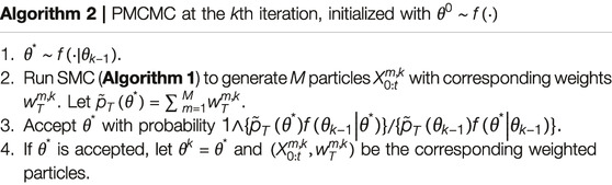
Algorithm 2. PMCMC at the kth iteration, initialized with ${\theta }^0\sim f(\cdot )$

 The assumption of a single fully specified HMM in particle filter is often too restrictive in applications since the model parameters are usually unknown and also need to be estimated sequentially from the observed data. A standard method to estimate unknown parameters is to assume a prior distribution for the unknown parameter vector and to use the Markov chain Monte Carlo (MCMC) to estimate the posterior distribution. Authors of reference [15] carried out this method for time-homogeneous Markov chains $X_t\sim p_{\theta }(\cdot |X_{t-1})$ for $t\mathrm{⩾}1$ and $X_0\sim p_{\theta }(\cdot )$, with latent states $X_t$ and observations $Y_t\sim g_{\theta }(\cdot |X_t)$, in which θ is an unknown parameter with a prior density function $\pi (\cdot )$ with respect to some measure ${\nu }_{\mathit{\theta }}$ on the parameter space $\text{Θ}$. The posterior density of $\left(\theta ,X_{0:T}\right)$ given $Y_{1:T}$ is proportional to

$p_T\left(\vartheta ,x_{0:T}\right)=\pi \left(\vartheta \right)p_{\vartheta }\left(x_0\right){\displaystyle \prod }_{t=1}^T\left\{p_{\vartheta }\left(x_t|x_{t-1}\right)g_{\vartheta }\left(Y_t|x_t\right)\right\}.$

PMCMC uses SMC involving M particles (each of which consists of a sampled parameter and state trajectory) at every iteration k to construct an approximation ${\tilde{p}}_T$ to $p_T$ in a Metropolis–Hastings (MH) MCMC scheme that uses a proposal density $f(\cdot |{\theta }_{k-1})$ with respect to the measure $v_{\theta }$ to the sample ${\theta }_k$ at the kth iteration, as summarized in Algorithm 2. Chopin et al. (2013, Section 1.2) point out the difficulties in the asymptotic analysis of PMCMC as k becomes infinite. In particular, although the authors of reference [15] have shown that under some strong assumptions, PMCMC converges to a measure in total variation norm as $k\to \infty$, for fixed value of M, the limiting measure is not the target posterior distribution of $\left(\theta ,X_{0:t}\right)$. On the other hand, allowing M to approach $\infty$ with k would lead to an analytically intracAlgorithm scheme involving state spaces whose dimensions change with k. Authors of reference [16] propose the SMC² scheme to target heuristically the posterior distribution of $\left(\theta ,X_{0:t}\right)$ given $Y_{1:t}$$\left(1\mathrm{⩽}t\mathrm{⩽}T\right)$ as follows. It involves N θ-particles, which we will call “atoms,” and attaches to each atom θ a particle filter that propagates and resamples M particles (state trajectories $X_{0:t}^m$) generated by SMC (as in Algorithm 1 with the given θ). It carries out the MH iterations to determine if a candidate atom is accepted (as in Step (c) of Algorithm 2). For the N atoms ${\theta }_t^1,\dots ,{\theta }_t^N$ and their corresponding importance weights at time t generated in this way, if the degeneracy criterion in the study by the author of reference [17] is satisfied, carry out bootstrap resampling of the weighted parameter-particle set to replace it by an unweighted set, but no convergence theory as $k\to \infty$ is provided. Although MCMC methods with MH iterations are widely used computational tools in Bayesian inference on $\theta \in \text{Θ}$ that has prior density function with respect to some measure ${\nu }_{\theta }$, they do not have convergence rate guarantees in terms of the number of iterations to automate termination of the iterations. On the other hand, if the target density p, which is the posterior density of θ given $Y_{1:t}$, was known and easy to sample from, then the standard Monte Carlo approximation of $\mu :=E_p\left(\psi \left(\theta \right)\right)$ could be carried out by generating i.i.d. ${\theta }_1,\dots ,{\theta }_N$ from $p(\cdot )\text{d}m$ and using the sample average $\tilde{\mu }=N^{-1}{{{\displaystyle \sum }}^{\text{}}}_{n=1}^N\psi \left({\theta }_n\right)$ to estimate μ. Under the assumption $E_p\left({\psi }^2\left(\theta \right)\right)<\mathrm{\infty }$, the estimated standard error is ${\tilde{\sigma }}_N/\sqrt{N}$, and $\tilde{\mu }\pm N^{-1/2}{\tilde{\sigma }}_N{\zeta }_{1-\alpha /2}$ is an approximate $\left(1-\alpha \right)$-level confidence interval for μ, where ${\tilde{\sigma }}_N^2={\left(N-1\right)}^{-1}{{{\displaystyle \sum }}^{\text{}}}_{n=1}^N{\left(\psi \left({\theta }_n\right)-\tilde{\mu }\right)}^2$ and ${\zeta }_q$ is the qth quantile of the standard normal distribution. This follows from the classical central limit theorem and is very useful for determining N to ensure $\tilde{\mu }$ to be within some prescribed tolerance limit ϵ of μ: $N^{-1/2}{\tilde{\sigma }}_N{\zeta }_{1-\alpha /2}\mathrm{⩽}\mathit{ϵ}$ and has inspired Lai to develop, with his current Ph.D. students Huanzhong Xu, Michael Hongyu Zhu, and former Ph.D. student Hock Peng Chan, the following novel MCMC algorithm which is asymptotically equivalent to the oracle procedure that assumes known target density p and which they call MCMC with sequential state substitutions (MCMC-SS). As in MH, let f be a given function that is proportional to the target density. Let $\{q(\cdot |\gamma ):\gamma \in \text{Γ}\}$ be a family of positive proposal densities with respect to some measure m, where $\text{Γ}$ is a convex subset of ${\mathrm{ℝ}}^d$. MCMC-SS initializes by choosing ${\gamma }_0\in {\text{Γ}}^o$ and generating $\nu B$ i.i.d. ${\theta }_{\mathrm{1,0}}^1,\dots ,{\theta }_{\mathrm{1,0}}^{\nu };\dots ;{\theta }_{B,0}^1,\dots ,{\theta }_{B,0}^{\nu }$ from the proposal distribution $q(\cdot |{\gamma }_0)\text{d}m$, thereby forming the B disjoint sets ${\text{Θ}}_{b,0}=\left\{{\theta }_{b,0}^1,\dots ,{\theta }_{b,0}^{\nu }\right\}$. At the stage k, it uses the sequential substitution procedure SS$\left({\text{Θ}}_{b,k},{\mathit{w}}_k^b\right)$ in Algorithm 3 to update the atom set in the bth block and to assign the weight $w_{i,k}^b$ to the ith atom in ${\text{Θ}}_{b,k}$, $b=1,\dots ,B$. MCMC-SS estimates $\mu ={\mathcal{E}}_p\psi \left(\theta \right)$ by the following equation:

$\widehat{\psi }=\frac{1}{B\left(K-\kappa \right)}{\displaystyle \sum }_{b=1}^B{\displaystyle \sum }_{k=\kappa +1}^K{\widehat{\psi }}_{b,k},\text{ with }{\widehat{\psi }}_{b,k}=\frac{{{{\displaystyle \sum }}^{\text{}}}_{i=1}^{\nu }{w}_{i,k}^b\psi \left({\theta }_{i,k}^b\right)}{{{{\displaystyle \sum }}^{\text{}}}_{i=1}^{\nu }{w}_{i,k}^b},$

in which κ represents an initial burn-in period that is asymptotically negligible as $\kappa =o\left(K\right)$. In many applications, the parameter γ of the family of proposal densities is a function $\gamma :\mathcal{P}\to \text{Γ}$, where $\mathcal{P}$ is the space of probability measures on $\text{Θ}$. Assuming this framework, we now describe the choice of ${\gamma }_{b,k-1}$ in Algorithm 3. For $k\mathrm{⩽}\kappa$, let ${\gamma }_{b,k-1}={\nu }^{-1}{\displaystyle {\sum }_{\theta \in {\text{Θ}}_{b,k-1}}\gamma \left(\theta \right)}$, which is the mean of the empirical measure of the atoms in the bth block at the end of stage $k-1$. On the other hand, for $k>\kappa$, we pool across blocks by letting ${\gamma }_{k-1}=B^{-1}{{{\displaystyle \sum }}^{\text{}}}_{b=1}^B{\gamma }_{b,k-1}$, which we use as the modified ${\gamma }_{b,k-1}$ for all blocks. Therefore, after the burn-in period, we can carry out the update $\text{SS}\left({\text{Θ}}_{b,k}\right)$ in the order $b=1,\dots ,B$, so that if the candidate atom in SS(${\text{Θ}}_{b,k}$) is not used for block b, it can serve as candidate atom for the block $b+1$ ($\mathrm{⩽}B$), which then does not need to generate another random variable from $q(\cdot |{\gamma }_{k-1})$, an obvious advantage for high-dimensional and complicated states. Lai, Xu, Zhu, and Chan have developed a comprehensive asymptotic theory of MCMC-SS showing its asymptotic optimality with respect to computational and statistical criteria and have also derived consistent estimators of the standard errors for the Monte Carlo state/parameter estimates; see reference [18] for which the main results are summarized in the following that includes Algorithm 3. Moreover, Algorithm 3 that can be vectorized and parallelized and illustrate its applications to latent variable analysis with uncertainty quantification in image reconstruction and brain network development.

ALGORITHM 3

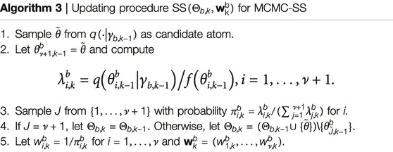
Algorithm 3. Updating procedure $\text{SS}\left({\text{Θ}}_{b,k},{\mathbf{w}}_{\text{k}}^{\text{b}}\right)$ for MCMC-SS

Theorem 2. Suppose${\mathcal{E}}_p{\psi }^2\left(\theta \right)$and there exist$\beta >\alpha >0$and$V:{\text{Θ}}^{\nu }\to [1,\infty )$such that for$\gamma :\mathcal{P}\to \text{Γ}$,

$\begin{array}{l}\underset{{\text{Θ}}^{\nu }}{{\displaystyle \int }}V\left(\mathit{\theta }\right)q\left({\theta }^1|{\gamma }_0\right)\dots q\left({\theta }^{\nu }|{\gamma }_0\right)\text{d}{m}^{\nu }\left(\mathit{\theta }\right)<\infty with \mathit{\theta }=\left({\theta }^1,\dots ,{\theta }^{\nu }\right),\text{ and}\\ \alpha V\left(\mathit{\theta }\right)\mathrm{⩽}\lambda \left(\tilde{\theta }|\gamma \left(\mathit{\theta }\right)\right)\mathrm{⩽}\beta V\left(\mathit{\theta }\right)\text{ for all }\mathit{\theta }\in {\text{Θ}}^{\nu }\text{ and }\tilde{\theta }\in \text{Θ},\end{array}$

where $\lambda \left(\tilde{\theta }|\gamma \right)=f\left(\tilde{\theta }|\gamma \right)/p\left(\tilde{\theta }\right)$.

(i) Let $G_{b,k}$ be the joint distribution of $\left({\theta }_{1,k}^b,\dots ,{\theta }_{\nu ,k}^b\right)$ and let $Q^{\nu }$ be the probability measure on ${\text{Θ}}^{\nu }$ that has the density of ν independent components each of which has density $q(\cdot |{\gamma }_f)$ with respect to m, where ${\gamma }_f=argmi{n}_{\gamma \in \text{Γ}}I(q_{\gamma }\parallel f)$ and $I(q\parallel f)={\mathcal{E}}_f\left\{\text{log}(q\left(\theta \right)/f\left(\theta \right))\right\}$ is the Kullback–Leibler divergence (or relative entropy) of q from the target density f in Algorithm 3 Then there exist positive constants a and c such that ${\Vert G_{b,k}-Q^{\nu }\Vert }_V\mathrm{⩽}c{e}^{-ak}$ for $1\mathrm{⩽}k\mathrm{⩽}K$, where $\parallel \cdot {\parallel }_V$ denotes the weighted total variation norm associated with the weight function V. Hence, after $k\succ \log B$ iterations, ${\displaystyle {\sum }_{b\mathrm{⩽}B}{\Vert G_{b,k}-Q^{\nu }\Vert }_V\to 0}$.

(ii) Let $N=B\left(K-\kappa \right)$ be the total number of atoms used to define the MCMC-SS estimate of $\tilde{\psi }$ of $\mu ={\mathcal{E}}_p\left(\psi \left(\theta \right)\right)$. Then as $K\to \infty$ and $B\to \infty$ such that $B=\mathcal{O}\left(K\right)$,

$\sqrt{N\nu }\left(\widehat{\psi }-\mu \right)\Rightarrow N\left(0,{\sigma }^2\right),$

where ${\sigma }^2=Va{r}_p\left(\psi \left(\theta \right)\right)$ and can be consistently estimated by:

${\widehat{\sigma }}^2=\frac{1}{B\left(K-\kappa \right)}{\displaystyle \sum }_{b=1}^B{\displaystyle \sum }_{k=\kappa +1}^K\frac{1}{\nu -1}{\displaystyle \sum }_{\theta \in {\text{Θ}}_{b,k}}{\left(\psi \left(\theta \right)-{\widehat{\psi }}_{b,k}\right)}^2.$

 As shown in reference [21], with probability approaching 1 by large k, the candidate atom $\tilde{\theta }$ in Algorithm 3 substitutes some existing atom in ${\text{Θ}}_{b,k-1}$. Hence, similar to the case of known target density p from which $\tilde{\theta }$ is sampled, the newly sampled atom features in the weighted average ${\widehat{\psi }}_{b,k}$. The reason we need the weighted average, with “importance sampling weights” $w_{i,k}^b$, is that for large k, the conditional distribution of ${\text{Θ}}_{b,k}$ given ${\text{Θ}}_{b,k-1}$ behaves like the ν-fold product measure $Q^{\nu }$ on ${\text{Θ}}^{\nu }$. This shows that importance sampling (likelihood ratio) weights $w_{i,k}^b$ are needed to convert Q to P and suggests the asymptotic optimality of $\widehat{\psi }$, which is the overall average of the $B\left(K-\kappa \right)$ estimates ${\widehat{\psi }}_{b,k}$, similar to $\widehat{\mu }$ that is described for the case of known p. Each random variable generated in the MCMC-SS scheme asymptotically contributes weight ${\left(N\nu \right)}^{-1}$ to (a) the estimate $\widehat{\psi }$ of μ and (b) the asymptotic variance of $\widehat{\psi }$. Theorem 2 shows that there is in fact considerable flexibility in the choice of the factors K (the number of iterations) and B (the number of blocks) in $N=B\left(K-\kappa \right)$ that determines the scaling factor in the central limit theorem, although the theorem highlights the case $B=\mathcal{O}\left(K\right)$ to emphasize that K should not be chosen too small relative to B. Reference [21] gives an application to uncertainty quantification in the following image reconstruction problem. Reference [22] propose to use MCMC methods “whenever the target measure has density with respect to a Gaussian process or Gaussian random field reference measure.” A wide range of applications involving such a framework considers Bayesian inference on a latent random field $\left\{u\left(x\right):x\in D\right\}\subset {\mathrm{ℝ}}^d$ generated by some stochastic partial differential equation (SPDE) in which D is a connected subset of ${\mathrm{ℝ}}^{d\text{'}}$, based on data generated by some nonlinear function of the random field. It is shown that after discretization and truncation to fit into this framework, the Radon–Nikodym derivative of the target measure P with respect to the reference measure Q has the following form:

$\left(dQ/dP\right)\left(u\right)\propto \text{exp}\left(-l\left(u\right)\right),$

for some real-valued function l, which [19] call “potential” in their substantive applications. The advantage of using a zero-mean Gaussian random field reference measure Q is that it is specified by the covariance operator $\mathcal{C}$ whose eigenvalues ${\lambda }_i$ and orthonormal eigenfunctions ${\varphi }_i$ yield the Karhunen–Loève expansion $u\left(x\right)={{{\displaystyle \sum }}^{\text{}}}_{i=1}^{\infty }{\xi }_i{\varphi }_i\left(x\right)$, with i.i.d. ${\xi }_i$ that are $N\left(0,{\lambda }_i^2\right)$ and ${{{\displaystyle \sum }}^{\text{}}}_{i=1}^{\infty }{\lambda }_i^2<\infty$. Reference [22] uses a random truncation τ with a sieve prior to convert the infinite-dimensional expansion to a finite sum $u\left(x\right)={{{\displaystyle \sum }}^{\text{}}}_{i=1}^{\tau }{\xi }_i{\varphi }_i\left(x\right)$. In addition, a discrete approximation of the random field $u\left(x\right)$ is used, with x taken over a mesh of width δ in each coordinate. MCMC-SS uses a parametric family of Gaussian proposal measures $Q\left(\gamma \right)$ instead of a single one by [22]. Putting $1/L\left(\theta \right)=\text{exp}\left(-l\left(u\left(x\right)\right)\right)$, we can also incorporate the random truncation τ and possibly also other random effects ρ into the state $\theta =\left(\tau ,{\zeta }_1,\dots ,{\zeta }_{\tau },\rho \right)$, where ${\zeta }_j=\mathcal{G}\left(u\left(x_j\right)\right)$, $j=1,\dots ,\tau$, and $\mathcal{G}$ is an operator associated with the SPDE and the discretization scheme for which $x_j$ belongs to a discrete subset of D. With this definition of θ, MCMC-SS uses the updating procedure described in Algorithm 3. Section 4.2 of [22] argues that simply applying MCMC to a discretized random field leads to a singular reference measure with respect to the target measure. However, the MCMC procedure used in [22] is the random walk Metropolis algorithm that involves the acceptance probability $a\left(u,v\right)=\text{min}\left\{1,\left(d{\eta }^{\text{*}}/d\eta \right)\left(u,v\right)\right\}$, where η is the measure defined by the transition kernel $q\left(u,v\right)$ of the MCMC algorithm (i.e., $v|u\sim q\left(u\right)$) and ${\eta }^{\text{*}}$ is the measure obtained by reversing the roles of u and v in the definition of η. Theorem 6.3 of [22] shows that after discretization, ${\eta }^{\text{*}}$ is singular with respect to η and therefore “all proposal moves are rejected with probability 1” for the random walk Metropolis algorithm, which proposes $v^{\left(k\right)}=u^{\left(k\right)}+\beta {\xi }^{\left(k\right)}$, with ${\xi }^{\left(k\right)}\sim N\left(0,C\right)$, and chooses $u^{\left(k+1\right)}=v^{\left(k\right)}$ with probability $a\left(u^{\left(k\right)},v^{\left(k\right)}\right)$, setting $u^{\left(k+1\right)}=u^{\left(k\right)}$ if $v^{\left(k\right)}$ is rejected. To get around this difficulty, [22] introduces a preconditioned Crank–Nicolson (pCN) adjustment, which proposes $v^{\left(k\right)}=\sqrt{1-{\beta }^2}{u}^{\left(k\right)}+\beta {\xi }^{\left(k\right)}$. Here, ${\beta }^2=8\delta /{\left(2+\delta \right)}^2$ and C is the covariance matrix (after truncation and discretization) of the covariance operator $\mathcal{C}$ for the Gaussian proposal measure. Because MCMC-SS does not involve η and ${\eta }^{\text{*}}$, it does not require the pCN adjustments; see reference [20] for details and further discussion. Making use of bounds on a weighted total variation norm of the difference between the target distribution and the empirical measure defined by the sample paths of the MCMC procedure, reference [21] has developed an asymptotic theory of the MCMC-SS estimates, as both K and N approach $\infty$, of functionals of the target distribution. This asymptotic theory includes asymptotic normality of the MCMC-SS estimates, provides consistent estimators of their standard errors, and establishes their asymptotic optimality by deriving certain oracle properties. Implementation via sequential Monte Carlo schemes called “particle filters” and parallelization is also given. In his Ph.D. thesis, Zhu who is a coauthor of [21] describes a numerically stable implementation of MCMC-SS that can be vectorized and parallelized, using Julia v0.62 [23] and the ArrayFire GPU library [24]. He also develops scalable implementations for high-dimensional states/parameters using differentiation through mixture distributions for stochastic gradient descent; see [25]. In the context of cortical organoids described in the first paragraph of Section 2, the target distribution is the posterior distribution of a precomputed feature of the organoid as a scaled-down model of the preterm human brain, conditional on the observations which are the 101 serial EEG recordings from 39 preterm infants. The uncertainty quantification [21] of the posterior distribution of a precomputed feature of cortical organoids provides a principled and systematic approach to the comparison of the feature between cortical organoids and the observations from the preterm infants, in contrast to the lack of uncertainty quantification for the approach and results of [1, pp. 8–9 and Fig. 4A, B, C, and D on p. 31] mentioned in the first paragraph of Section 2. Moreover, the methods of time–frequency analysis in the preceding subsection can be used to compute the predictive distribution of the feature of the cortical organoids given the observations, which is the same as the target distribution. The predictive distribution typically also involves an unspecified hyperparameter vector $\mathit{\theta }$, as in manifold learning of [14]. This corresponds to a Bayesian approach with prior densities belonging to a family of proposal densities $q\left(\mathit{\theta }|\gamma \right)$, in which $\gamma \in \text{Γ}$ indexes the family and $\text{Γ}$ is a convex subset of ${\mathrm{ℛ}}^d$. Reference [21] has shown that MCMC-SS eventually samples from $q(\cdot |{\gamma }_p)$ that has the smallest Kullback–Leibler divergence from $p(\cdot )$, and therefore from the target density if it belongs to $\{q(\cdot |\gamma ):\gamma \in \text{Γ}\}$.

3 Discussion and Concluding Remarks

Haddad and Lai actually initiated similar research forty years ago when they worked on cardiorespiratory patterns during sleep in a SIDS (Sudden Infant Death Syndrome) project at Columbia University’s Pediatrics Department; see reference [26] which describes the study population consisting of 12 infants “with one or more episodes of aborted SIDS” (four of whom had siblings who died of SIDS), and 19 normal infants, all born full-term except for one aborted SIDS infant born at 37 weeks of gestation. After describing the study design and methods of statistical analysis, the authors of reference [26] presented results on total tidal volume (Vt), respiratory cycle time (Ttot), and increase in Vt/Ttot resulting from 2% increase in CO₂ concentration in the sleeping chamber, comparing aborted SIDS to normal infants in both REM (rapid eye movement) and quiet sleep. Because of the inability to induce stress such as loaded breathing as in reference [27, 28], animal models involving sheep, puppies, and dogs were used; see also [29]. In particular, the authors of reference [24] “studied diaphragmatic muscle function during inspiratory flow resistive loaded breathing” in 6 unanesthetized sheep over periods of 6–8 months. Data were collected (baseline) and after application of the loads that were sustained for up to 90 min. Loads were divided into mild (<50 cm H₂O$\cdot$${\mathrm{l}}^{-1}$s), moderate (50–150 cm H₂O$\cdot$${\mathrm{l}}^{-1}$s), and severe (>150 cm H₂O$\cdot$${\mathrm{l}}^{-1}$s). They found that “1) the diaphragm is capable of generating large pressure for prolonged periods with no evidence of fatigue, 2) with very high inspiratory resistive loads mechanical failure of the diaphragm can occur, 3) diaphragmatic fatigue is associated with acute hypercania and therefore failure of the entire respiratory pump, and 4) a decrease in integrated EMG (iEMG) and a concomitant shift in the EMG power spectral density toward lower frequencies precede the mechanical failure of the diaphragm.” Thus, similar to the power spectral density of the EEG signal in the first paragraph of Section 2, [27] uses a shift of the power spectrum of the EMG toward lower frequencies to identify the onset of diaphragmatic muscle fatigue in adult sheep. The frontier methods of time–frequency analysis in Section 2.1 are therefore also relevant to the problem of diaphragmatic muscle fatigue and rhythmic variations in cardiorespiratory signals studied by Haddad and Lai forty years ago. Pointing out that in the 1980s “investigators from various disciplines focused their efforts on finding out whether SIDS is related to hypoxia or anoxia (acute or chronic) before death and whether this relation is responsible for events leading to death”, Haddad [30], reviewed “studies in the recent past” from various fields—epidemiology, physiology of infant death and SIDS, pathology of the airway, and animal studies. Although “most of the evidence accumulated so far, including that obtained in the past two years, is circumstantial,” he concluded that “SIDS was little understood for many years until, over the past few years, its basic underlying genetic defect was better characterized (from recent animals and human studies), and light could finally be seen at the end of the tunnel,” again linking genetics and feedback mechanisms to see this light, as in the exemplary work of Hall, Rosbach, and Young on the circadian rhythm. Combining various clues and insights from different areas/studies via an empirical Bayes model is the capability of the frontier approach described in Section 2.2; see Sections 3.6.3, 5.4, 6.2.3 and 7.4 of reference [31] on postmarketing monitoring of medical product safety.

A related direction of our ongoing research is to combine several biomedical signals, which form a multivariate time series, thereby providing a more holographic view of a human subject. For example, in an intensive care unit, PPG can be combined with EEG, EMG, respiratory, and other signals to evaluate a patient’s health status. Wu and his collaborators have applied in [32,33] a combination of ST and EEG channels to study sleep dynamics and an “interpretable machine learning algorithm” to assess consistency of sleep-stage scoring rules across multiple sleep centers. How to utilize available information from multiple centers is a sensor fusion problem. We are currently combining recent advances in sensor fusion with those in TFA to develop integrated statistical analysis of the multivariate time series of multiple biomedical signals.

Data Availability Statement

The original contributions presented in the study are included in the article/Supplementary Material, and further inquiries can be directed to the corresponding author.

Author Contributions

All authors listed have made a substantial, direct, and intellectual contribution to the work, and approved it for publication.

Funding

TL’s research was supported by the National Science Foundation under DMS-1811818. GH’s research was supported by the National Institutes of Health under 1R01HL146530 and 1R21NS111270. AM’s research was supported by the National Institutes of Health under DP2-OD006495.

Conflict of Interest

The authors declare that the research was conducted in the absence of any commercial or financial relationships that could be construed as a potential conflict of interest.

Acknowledgments

We thank TL’s research assistant Chenru Liu at Stanford University for her valuable contributions to the preparation, timely submission, and revision of the paper. We also thank the reviewers whose innovative comments and suggestions have resulted in substantial improvement of the presentation.

References

1. Trujillo, CA, Gao, R, Negraes, PD, Gu, J, Buchanan, J, Preissl, S, et al. Complex Oscillatory Waves Emerging from Cortical Organoids Model Early Human Brain Network Development. Cell Stem Cell (2019). 25(4):558–69. doi:10.1016/j.stem.2019.08.002

PubMed Abstract | CrossRef Full Text | Google Scholar

2. Wu, H-T. Current State of Nonlinear-type Time-Frequency Analysis and Applications to High-Frequency Biomedical Signals. Curr Opin Syst Biol (2020). 23:8–21. doi:10.1016/j.coisb.2020.07.013

CrossRef Full Text | Google Scholar

3. Shelley, KH. Photoplethysmography: beyond the Calculation of Arterial Oxygen Saturation and Heart Rate. Anesth Analg (2007). 105:531–6. doi:10.1213/01.ane.0000269512.82836.c9

PubMed Abstract | CrossRef Full Text | Google Scholar

4. Cicone, A, and Wu, HT. How nonlinear-type time-frequency analysis can help in sensing instantaneous heart rate and instantaneous respiratory rate from photoplethysmography in a reliable way. Front Phy (2017). 8:701.

CrossRef Full Text | Google Scholar

5. Wardhan, R, and Shelley, K. Peripheral venous pressure waveform. Curr Opin Anesthesiol (2009). 22:814–821.

PubMed Abstract | CrossRef Full Text | Google Scholar

6. Wu, HT, Alian, A, and Shelley, KH. A new approach to complicated and noisy physiological waveforms analysis: peripheral venous pressure waveform as an example. J Clin Monit Comput (2020). 1–17.

PubMed Abstract | CrossRef Full Text | Google Scholar

7. Flandrin, P. Wavelet Analysis and its Applications (1999). p. 10.Time-frequency/time-scale Analysis

Google Scholar

8. Huang, NE, Shen, Z, Long, RS, Wu, HH, Zheng, Q, et al. The Empirical Mode Decomposition and the hilbert Spectrum for Nonlinear and Non-stationary Time Series Analysis. Proc R Soc Lond A (1998). 454:903–95. doi:10.1098/rspa.1998.0193

CrossRef Full Text | Google Scholar

9. Nahon, M. Phase Evaluation and segmentationPhD Thesis. New Haven: Yale University (2000).

10. Daubechies, I, Lu, J, and Wu, H-T. Synchrosqueezed Wavelet Transforms: an Empirical Mode Decomposition-like Tool. Appl Comput Harmonic Anal (2011). 30:243–61. doi:10.1016/j.acha.2010.08.002

CrossRef Full Text | Google Scholar

11. Daubechies, I, Wang, Y, and Wu, H-t. ConceFT: Concentration of Frequency and Time via a Multitapered Synchrosqueezed Transform. Phil Trans R Soc A (2016). 374:20150193. doi:10.1098/rsta.2015.0193

PubMed Abstract | CrossRef Full Text | Google Scholar

12. Mallat, S. Group Invariant Scattering. Comm Pure Appl Math (2012). 65:1331–98. doi:10.1002/cpa.21413

CrossRef Full Text | Google Scholar

13. Lin, C-Y, Su, L, and Wu, H-T. Wave-Shape Function Analysis. J Fourier Anal Appl (2018). 24:451–505. doi:10.1007/s00041-017-9523-0

CrossRef Full Text | Google Scholar

14. Wang, S-C, Wu, H-T, Huang, P-H, Chang, C-H, Ting, C-K, and Lin, Y-T. Novel Imaging Revealing Inner Dynamics for Cardiovascular Waveform Analysis via Unsupervised Manifold Learning. Anesth Analgesia (2020). 130:1244–54. doi:10.1213/ane.0000000000004738

PubMed Abstract | CrossRef Full Text | Google Scholar

15. Gordon, NJ, Salmond, DJ, and Smith, AFM. Novel Approach to Nonlinear/non-Gaussian Bayesian State Estimation. IEE Proc F Radar Signal Process UK (1993). 140:107–13. doi:10.1049/ip-f-2.1993.0015

CrossRef Full Text | Google Scholar

16. Liu, JS. Monte Carlo Strategies in Scientific Computing. 2nd ed. New York: Springer (2008).

17. Chan, HP, and Lai, TL. A General Theory of Particle Filters in Hidden Markov Models and Some Applications. Ann Stat (2013). 41(6):2877–904. doi:10.1214/13-aos1172

CrossRef Full Text | Google Scholar

18. Lai, TL Recursive Particle Filters for Joint State and Parameter Estimation in Hidden Markov Models with Multifaceted Applications. In: Proceedings of the 8th ICCM. Boston: International of Press; (2021) in press

Google Scholar

19. Chopin, N. A Sequential Particle Filter Method for Static Models. Biometrika (2002). 89(3):539–52. doi:10.1093/biomet/89.3.539

CrossRef Full Text | Google Scholar

20. Cotter, SL, Roberts, GO, Stuart, AM, and White, D. MCMC Methods for Functions: Modifying Old Algorithms to Make Them Faster. Stat Sci (2013). 28:424–46. doi:10.1214/13-sts421

CrossRef Full Text | Google Scholar

21. Andrieu, C, Doucet, A, and Holenstein, R. Particle Markov Chain Monte Carlo Methods. J R Stat Soc Ser B (2010). 72(3):269–342. doi:10.1111/j.1467-9868.2009.00736.x

CrossRef Full Text | Google Scholar

22. Chopin, N, Jacob, PE, and Papaspiliopoulos, O. SMC2: an Efficient Algorithm for Sequential Analysis of State Space Models. J R Stat Soc Ser B (2013). 75(3): 397–426. doi:10.1111/j.1467-9868.2012.01046.x

CrossRef Full Text | Google Scholar

23. Bezanson, J, Edelman, A, Karpinski, S, and Shah, VB. Julia: A Fresh Approach to Numerical Computing. SIAM Rev (2017). 59(1):65–98. doi:10.1137/141000671

CrossRef Full Text | Google Scholar

24. Yalamanchili, P, Arshad, U, Mohammed, Z, Garigipati, P, Entschev, P, Kloppenborg, B, et al. ArrayFire - A High Performance Software Library for Parallel Computing with an Easy-To-Use API (2015).

25. Zhu, M. Ph.D. Dissertation in Computer Science. Stanford University (2021). doi:10.1145/3450439.3451855Improving and Accelerating Particle-Based Probabilistic Inference

CrossRef Full Text | Google Scholar

26. Haddad, GG, Leistner, HL, Lai, TL, and Mellins, RB. Ventilation and Ventilatory Pattern during Sleep in Aborted Sudden Infant Death Syndrome. Pediatr Res (1981). 15(5):879–83. doi:10.1203/00006450-198105000-00011

PubMed Abstract | CrossRef Full Text | Google Scholar

27. Bazzy, AR, and Haddad, GG. Diaphragmatic Fatigue in Unanesthetized Adult Sheep. J Appl Physiol (1984). 57(1):182–90. doi:10.1152/jappl.1984.57.1.182

CrossRef Full Text | Google Scholar

28. Haddad, GG, Jeng, HJ, Bazzy, AR, and Lai, TL. Within-breath Electromyographic Changes during Loaded Breathing in Adult Sheep. J Appl Physiol (1986). 61(4):1316–21. doi:10.1152/jappl.1986.61.4.1316

CrossRef Full Text | Google Scholar

29. Haddad, GG, Jeng, HJ, Lee, SH, and Lai, TL. Rhythmic Variations in R-R Interval during Sleep and Wakefulness in Puppies and Dogs. Am J Physiology-Heart Circulatory Physiol (1984). 247(1):H67–H73. doi:10.1152/ajpheart.1984.247.1.h67

CrossRef Full Text | Google Scholar

30. Haddad, GG. The Multifaceted Sudden Infant Death Syndrome. Curr Opin Pediatr (1992). 4(3):426–30. doi:10.1097/00008480-199206000-00006

CrossRef Full Text | Google Scholar

31. Chen, J, Heyse, JF, and Lai, TL. Medical Product Safety Evaluation: Biological Models and Statistical Methods. Boca Raton FL: Chapman & Hall/CRC (2018). doi:10.1201/9781351021982

CrossRef Full Text

32. Liu, GR, Lo, YL, Malik, J, Sheu, YC, and Wu, HT. Diffuse to Fuse EEG Spectra–Intrinsic Geometry of Sleep Dynamics for Classification. Biomed Signal Process Control (2019). 55(5):101576.

Google Scholar

33. Liu, G-R, Lin, T-Y, Wu, H-T, Sheu, Y-C, Liu, C-L, Liu, W-T, et al. Large-scale Assessment of Consistency in Sleep Stage Scoring Rules Among Multiple Sleep Centers Using an Interpretable Machine Learning Algorithm. J Clin Sleep Med (2021). 17(2):159–66. doi:10.5664/jcsm.8820

CrossRef Full Text | Google Scholar