Entrainment Dynamics Organised by Global Manifolds in a Circadian Pacemaker Model

1 Introduction

The function of the circadian timekeeping system is to align an organism’s physiology and behaviour with the daily environmental cycles conferred by Earth’s rotation. Alignment is achieved by endogenous circadian oscillators with periods close to, but not exactly, 24 h synchronising to external 24 h periodic signals, such as the light/dark cycle, in a process called entrainment. Properties of both the internal oscillator and the external forcing signal, such as intrinsic period and light intensity, combine to determine the stable phase of entrainment. For example, circadian clocks with long intrinsic periods can lead to delayed sleep phase syndrome (DSPS), a disorder where patients tend to be unable to fall asleep until late at night and have difficulty waking up in the morning. Bright light therapy can help to advance the entrained phase of DSPS patients so that their hormonal rhythms, sleep-wake patterns, and peak performance times are more in line with societal norms [1].

Failure to achieve entrainment can occur if the mismatch between the periods of the intrinsic oscillator and the external forcing is sufficiently large and the forcing signal is sufficiently weak. In non-24 h sleep-wake disorder (non-24), patients are unable to establish a stable 24 h sleep-wake rhythm [2–5]. Non-24 is common in blind people that do not have any light perception, leading to sleep-wake rhythms with the period of their intrinsic circadian clock. Since the intrinsic period of most people is greater than 24 h, this results in sleep-wake patterns where the phase of sleep onset progressively drifts later in the day from one day to the next. Non-24 is also experienced by sighted individuals where the combination of a short or long intrinsic period and a reduced sensitivity to light renders them unable to entrain to 24 h cycles.

Transient misalignment of circadian rhythms occurs when there is an abrupt shift in the phase of environmental cycles. After rapid travel across time zones, it can take several days for the circadian clock to establish a stable phase relationship with the light/dark cycle in the new time zone. During the re-entrainment process, travelers may experience insomnia, daytime sleepiness, gastrointestinal issues, and other symptoms collectively known as jet lag. Circadian misalignment and associated health problems can also be caused by a change in work patterns, for example, when a worker transitions from day shift to night shift or vice versa. In particular, rotating or permanent night-shift workers have increased incidence of cardiovascular disease and cancer compared to permanent day shift workers [6]. Furthermore, night shift workers that are not entrained to a permanent night shift work schedule exhibit decreased alertness and performance levels relative to entrained night shift workers [7].

Mathematical modeling and tools from dynamical systems theory can be used to gain insight into circadian rhythm sleep disorders and the re-entrainment process following shifts in the light/dark cycle [8, 9]. The circadian clock is a complex system consisting of cellular oscillators and network interactions within and across brain regions and tissues throughout the body. Mathematical models have been developed to describe the circadian system at various levels, including detailed models of the transcription/translation feedback loops underlying intracellular molecular clocks and models of the electrical activity of the suprachiasmatic nucleus—a network of ∼20,000 neurons in the hypothalamus that serves as the brain’s master circadian timekeeper. We refer the reader to [10, 11] for reviews of biochemical and electrophysiological circadian models. Other modelers have focused less on the cellular details and instead have tried to capture the behavior of the circadian system at the level of the whole organism (see [12] for a review). One such effort is the Forger–Jewett–Kronauer (FJK) model, a low-dimensional model of the human circadian system consisting of a central limit cycle oscillator that responds to light via processing by the retina [13]. This model is based on experiments measuring how the amplitude and phase of circadian rhythms in human subjects respond to light pulses. It has been extensively validated in laboratory and field conditions, making it an attractive choice for simulating jet lag and other perturbations to the circadian system [14]. Here, we use dynamical systems tools to analyse the entrainment dynamics of a reduction to the original FJK model.

The remainder of the manuscript is organised as follows. In Section 2, we consider the FJK model equations and then introduce the two-dimensional version of the model that we use in the present study. In Section 3, we characterise the bifurcations that lead to loss of entrainment when key parameters are varied and discuss these results in the context of non-24. In Section 4, we compute invariant manifolds of fixed points for a 24 h stroboscopic map constructed from the model. We show that these manifolds are able to explain the dynamics of a rapid re-entrainment phenomenon that has been previously observed under certain conditions in simulations and experiments. In Section 5, we illustrate how the manifolds organise the dynamics of re-entrainment following transitions between day and night shift work schedules. Finally, in Section 6, we discuss how our results relate to previous studies on the dynamics of circadian entrainment.

2 The Forger–Jewett–Kronauer Model

In 1990, Kronauer introduced a mathematical model of the human circadian pacemaker that reproduces many general features of how the circadian clock responds to light exposure in laboratory experiments [15]. Kronauer’s original model has subsequently been revised and extended to account for additional data on the effects of light observed in phase resetting experiments [16–18]. These models consist of a limit cycle oscillator, based on the Van der Pol equations, combined with a model of retinal light processing. Although these models are simplified descriptions of the human circadian system, they have become a widely-used tool for predicting circadian phase and have been carefully validated under a range of conditions [19–21]. Here we utilise the Forger–Jewett–Kronauer (FJK) version of the model [13]. This three-dimensional system of ordinary differential equations with external periodic forcing takes the following form:

$\dot{A}=\frac{\pi }{12}\left(\mu \left(A-q{A}^3\right)-C\left[{\left(\frac{24}{\rho {\tau }_c}\right)}^2+kB\right]\right),(1)$

$\dot{C}=\frac{\pi }{12}\left(A+B\right),(2)$

$\dot{n}=\alpha \left[I\right]f\left(t\right)\left(1-n\right)-\beta n(3)$

$B=G\alpha \left[I\right]f\left(t\right)\left(1-n\right)\left(1-KC\right)\left(1-KA\right),(4)$

$\alpha \left[I\right]={\alpha }_0{\left[\frac{I}{I_0}\right]}^p,(5)$

where the dots indicate derivatives with respect to time. The variable C captures daily fluctuations in core body temperature, A is a phenomenological auxiliary variable, and $n\in \left[\mathrm{0,1}\right]$ describes the activity of the phototransduction pathway that drives the circadian system in response to light input of intensity I with activation rate α and decay rate β. Equations 1,2 include modifications to the Van der Pol oscillator that scale the amplitude and adjust the period. The parameter ${\tau }_c$ represents an individual’s intrinsic circadian period; the correction factor ρ ensures that the model oscillation period equals ${\tau }_c$ for simulations in the absence of light $(I=0)$. The amplitude recovery term $\left(A-q{A}^3\right)$ yields a limit cycle amplitude of 1.0 in the absence of light. The parameter μ describes the rate of growth and decay of perturbations away from the limit cycle representing an entrained (24 h) circadian rhythm. The variable B, which is scaled by the gain parameter G, modulates the oscillator’s sensitivity to light in accordance with known circadian rhythms in human visual sensitivity [17]. The function α scales the light intensity with respect to a basal value $I_0$, a sensitivity exponent p, and a gain parameter ${\alpha }_0$ that was fitted to data on experiments with light stimuli over the photopic range [18]. The parameter K determines the shape of the phase response curve (PRC) to light, with positive values biasing the PRC to phase delays as observed in experiments [22]. Note that the impact of B on the auxiliary variable is scaled by a parameter $k<1$. Finally, $f\left(t\right)$ is a periodic function with a period of 24 h that, when combined with α, represents the light/dark cycle. In this paper, we assume that f is a square-wave with duty cycle $N\in \left[\mathrm{0,24}\right]$, shifted by an amount $t_{\text{s}}\in \left[\mathrm{0,24}\right]$:

$f\left(t\right)=\{\begin{array}{cc}1,& \left(t-t_{\text{s}}\right)\text{mod}24<N,\\ 0,& \text{otherwise},\end{array}(6)$

where N represents the number of hours of light in a 24 h interval.

In the absence of light (i.e., with $N=0$ or $I=0$), the system Eqs. 1–5 supports a stable limit cycle solution with period ${\tau }_c$. For appropriate choices of system and forcing parameters, the system can be entrained to a 24 h period orbit; example simulations using the default parameter values given in Table 1 are shown in Figures 1A–C. Throughout the paper, we will explore the ability of the system to entrain to such a 24 h cycle, and the consequences of perturbing trajectories away from the limit cycle representing this entrained solution, for example, in response to shift work.

TABLE 1

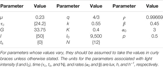
TABLE 1. Default parameter values used in analysis and model simulations.

FIGURE 1

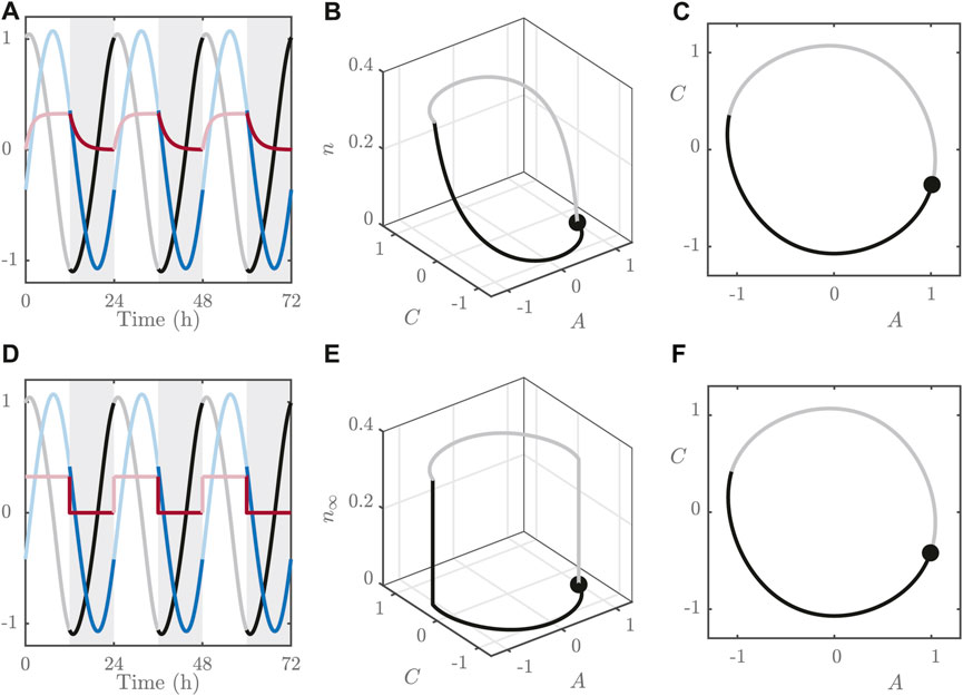
FIGURE 1. (A–C): Simulations of the FJK model Eqs 1–5 for $N=12$, ${\tau }_c=24.2$ with $I=50$. (D–F): Simulations of the 2D version of the FJK model using (Eq. 8) in place of (Eq. 4). (A) + (D): Time series of A (black), C (blue), and n (red). The shaded regions indicate where $f\left(t\right)=0$, whereas $f\left(t\right)=1$ in the unshaded regions. (B) + (E): Stable entrained limit cycle. The dark portion of the orbit corresponds to the interval in which $f\left(t\right)$ = 0. The marker shows the point along the orbit where f changes from 0 to 1. (C) + (F): Projection of panels (B, E), respectively, into the $\left(A,C\right)$ plane.

The dynamics for n are significantly faster than those for A and C, as can be seen in the time series in Figure 1. This means that n rapidly adopts its steady state value:

$n_{\infty }\left(I\right)=\frac{f\left(t\right)\alpha \left(I\right)}{\beta +\alpha \left(I\right)}.(7)$

This observation allows us to approximate the full, three variable system with a 2-dimensional version by replacing Eq. 4 with

$B=G\alpha \left[I\right]f\left(t\right)\left(1-n_{\infty }\left[I\right]\right)\left(1-\mathrm{K}C\right)\left(1-\mathrm{K}A\right),(8)$

where $n_{\infty }$ has been substituted for n. To demonstrate the validity of this reduced model, we plot in Figures 1D–F a comparison of the full system with the one obtained by replacing n by $n_{\infty }\left(I\right)$. Reduction of the system to a two variable approximation facilitates analysis of the underlying dynamics, as we shall later elucidate.

The effect of changing shift work patterns, or of the jet lag induced by travelling across time zones (assuming variation in longitude only), can be modelled by changing $t_{\text{s}}$ and observing how trajectories return to the stable limit cycle. The severity of the effect of such perturbations can be measured by the entrainment time, that is, the duration required for trajectories starting from arbitrary initial points to converge to the stable orbit (we provide a more precise definition in Section 4) as the phase of the circadian oscillator with respect to the external forcing is varied. In Figures 2A,B, we plot re-entrainment times obtained by choosing initial conditions at regular phase shifts along the entrained limit cycle. For each point we change $t_{\text{s}}$ instantaneously from its reference value by the amount indicated on the x-axis, $\text{Δ}{t}_{\text{s}}$, and compute the time taken for the resulting trajectory to converge back to the limit cycle.

FIGURE 2

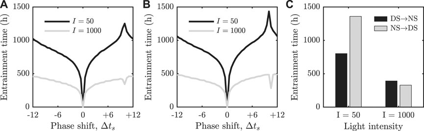
FIGURE 2. (A) + (B): Re-entrainment times as a function of the shift in the phase of the external forcing. The FJK model is shown in panel (A) and our two dimensional reduction is shown in panel (B). For $I=50$, we observe a peak in the re-entrainment time at around a +10.5 h shift. For $I=1000$, we now observe a local minimum, rather than a global maximum, in re-entrainment time for a +10.5 h shift in both models. (C): Re-entrainment times following transitions from day shift to night shift (DS$\to$NS) and from night shift to day shift (NS$\to$DS) in the 2D model.

Similarly to results reported in [23–26], we observe that there is a pronounced peak in the re-entrainment for $I=50$ for $\text{Δ}{t}_{\text{s}}\approx +10.5$, which suggests the existence of a “worst” shift in circadian phases. Interestingly, for higher light intensities, this global maximum in re-entrainment time is replaced by a local minimum, suggesting a change in dynamics near this value of $\text{Δ}{t}_{\text{s}}$. We remark here, that whilst we demonstrate this transition (from global maximum to local minimum) under variation of I, similar observations can be made for other system parameters, such as G or ${\alpha }_0$. This phenomenon has implications for jet lag (where $\text{Δ}{t}_{\text{s}}=+10$ corresponds to traveling 10 time zones in the eastward direction) and also for workers rotating between day and night shifts. We demonstrate in Figure 2C that at low light intensity, rotating from nights to days is more difficult than rotating from days to nights, whereas at high light intensity days to nights is more difficult than nights to days. The primary goals of this paper are to understand this transition and to establish where and how entrainment to a stable 24 h rhythm is lost.

3 Bifurcation Analysis

The behaviour of dynamical systems in general is organised by invariant sets in phase space and their associated manifolds. For periodically forced systems, these invariant sets typically take the form of periodic orbits, where we note that there may be many such objects in the full phase space. With this in mind, we aim to find periodic orbits of the two variable FJK model (hereby referred to as the 2D model) for the default parameter values; see Table 1. In particular, we seek to identify bifurcations in the number of periodic orbits since these transitions are relevant to understanding the dynamics of the entrainment process. Hence, we proceed to probe the bifurcation structure of the 2D model, using the methodology detailed in the Supplementary Material S1.

3.1 Variation of Light Intensity

We first perform bifurcation analysis in the light intensity parameter I and display the results in Figure 3. The bifurcation diagram in Figure 3A shows the branches of solutions under variation of I and we identify two fold bifurcations (around $I\approx 2.1$ and $I\approx 118.6$), which we label $I_{{\text{F}}_1}$ and $I_{{\text{F}}_2}$, respectively. For $I>I_{\text{F}2}$, we find that the only invariant set in the forced system is a stable limit cycle, the time series of which is shown in Figure 3B, and so all trajectories will converge to this orbit. For $I<I_{\text{F}1}$, there are no stable periodic orbits, and trajectories undergo quasiperiodic motion, highlighting the difficulty to entrain to a 24 h rhythm under extremely low light intensities. For intermediate values of $I_{\text{F}1}<I<I_{\text{F}2}$, the system exhibits three periodic orbits, one of which is stable and one of which is fully unstable, with the remaining orbit being of saddle type. These orbits are shown as time series in Figure 3C, in the full $\left(A,C,t\right)$ space in Figure 3D, and projected onto the plane of zero phase (of the light/dark cycle, i.e., the time at which f switches from 0 to 1) in Figure 3E. In this case, trajectories will ultimately converge to the stable periodic orbit, but the unstable limit cycles and their manifolds play an important role in organising how this occurs, as we shall discuss in Section 4.

FIGURE 3

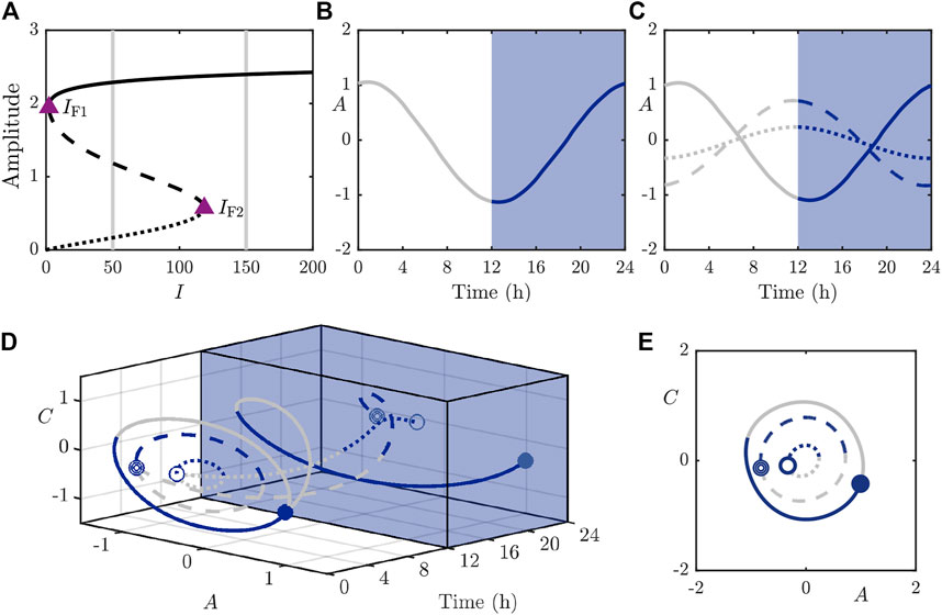
FIGURE 3. The stable (solid), saddle (dashed), and fully unstable (dotted) periodic orbits in the 2D model. (A): Bifurcation diagram of the periodic orbits under variation of I with other parameters as in Table 1. Purple triangles mark folds of periodic orbits at approximately $I_{\text{F}1}\approx 2.1$ and $I_{\text{F}2}\approx 118.6$. The vertical grey lines show the values of I used in panels (B) and (C). (B–C): Time series plots of the orbits over a 24 h period for $I=150$ [panel (B)], and $I=50$ [panel (C)]. Grey portions of the orbits correspond to $f\left(t\right)=1$, and navy portions correspond to $f\left(t\right)=0$ (shaded). (D–E): Orbits for $I=50$, as shown in panel (C), plotted over a 24 h period. The projection of these orbits onto a plane at zero phase of the forcing cycle [i.e., where $f\left(t\right)$ switches from 0 to 1] is shown on the front-facing surface [Time = 0 h] of panel (D) and in this $\left(A,C\right)$-plane alone in panel (E). The markers show the location of the periodic orbits at the zero phase of the forcing cycle.

3.2 Variation of Day Length

In addition to light intensity, the day length, expressed by the parameter N, also influences the number and type of periodic orbits supported by the system, as illustrated in Figures 4A–C. For $I=50$, the fully unstable limit cycle is disconnected from the branch of saddle and stable orbits; see Figure 4A. The isola formed by these latter branches is bounded by two fold bifurcations around $N_{\text{F}1}\approx 2.4$ and $N_{\text{F}4}\approx 23.5$, using similar notation as before. Thus, if the day length becomes too long or too short (as would be expected in polar regions), the circadian rhythm cannot be entrained to a 24 h rhythm. For higher values of I, the branch of fully unstable orbits merges with the branch of saddle orbits via a cusp bifurcation, leading to the formation of two more fold bifurcations. This scenario is highlighted in Figure 4B for $I=150$, where the additional folds occur at $N_{\text{F}2}\approx 9.3$ and $N_{\text{F}3}\approx 16.1$. For $N_{\text{F}2}<N<N_{\text{F}3}$, the stable periodic orbit is the only solution to the system. As I is increased further, the interval over N for which this is true grows (as shown in Figure 4C for $I=1000$), highlighting that higher light intensities facilitate entrainment to a 24 h rhythm.

FIGURE 4

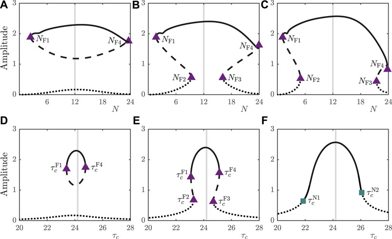
FIGURE 4. (A–C): Bifurcation diagrams of the 2D model under variation in N for $I=50$ [panel (A)], $I=150$ [panel (B)], and $I=1000$ [panel (C)]. Depicted are the amplitudes ($L^2$-norm) of the stable (solid), saddle (dashed), and fully unstable (dotted) periodic orbits. The vertical grey lines mark the default parameter value of $N=12$. (D–F): Bifurcation diagrams of the 2D model under variation in ${\tau }_c$ for $I=50$ [panel (D)], $I=150$ [panel (E)] and $I=1000$ [panel (F)]. The vertical lines mark ${\tau }_c=24.2$ in each panel. Fold bifurcations are indicated by purple triangles. Neimark–Sacker bifurcations are indicated by teal squares.

3.3 Variation of Natural Period

As well as considering properties of the external environment such as light intensity and day length, it is pertinent to consider the influence of intrinsic properties of the circadian oscillator on entrainment. The natural period, ${\tau }_c$, is of particular note since it can be directly measured and has been shown to affect individual’s entrainment properties and daily cycle habits, such as their chronotype [27]. To this end, we show in Figures 4D–F the branches of solutions under variation of ${\tau }_c$ for the same I values as in Figures 4A–C. We observe a similar structure between the two bifurcation diagrams, namely, that for low I values, as in Figure 4D, there is an isola structure similar to that in Figure 4A, but over a much smaller range of ${\tau }_c$. For higher I values, as seen by comparing Figure 4E with Figure 4B, there is a range over ${\tau }_c$ for which the system possesses only the stable periodic orbit, whilst for ${\tau }_c$ values either side of this region, all three aforementioned solutions are present. For the highest value of $I=1000$, as in Figure 4F, the stable periodic orbits destabilise via Neimark–Sacker bifurcations, rather than folds. This distinction in bifurcation type, whilst subtle, can have a significant effect on entrainment beyond the bifurcation point, as we shall discuss in Section 3.4.

3.4 Behaviour Near the Bifurcations

In Figures 4D–F, we observe that the type of bifurcation leading to loss of stability of the entrained orbit under variation of ${\tau }_c$ changes as I increases, switching from a fold to a Neimark–Sacker bifurcation. Following both of these bifurcation types, the system no longer possesses a stable period 1 orbit. In both scenarios, trajectories undergo torus-like behaviour, however, the manner in which they do so differs. This observation has particular significance for people with non-24 h sleep/wake cycles, which can be observed by analysing the phase dynamics of the quasiperiodic motion. In Figure 5, we show the dynamics of the system just past the fold bifurcations shown in Figure 4D (the top row shows dynamics for ${\tau }_c<{\tau }_c^{\text{F}1}$, where ${\tau }_c^{\text{F}1}$ corresponds to the left-most fold, whilst the bottom row displays dynamics for ${\tau }_c>{\tau }_c^{\text{F}4}$, where ${\tau }_c^{\text{F}4}$ corresponds to the right-most fold). The torus-like behaviour in both cases is evident from the modulation of the amplitude of the oscillations in C in Figures 5A,D.

FIGURE 5

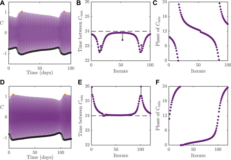
FIGURE 5. Dynamics of the 2D model with $I=50$ at ${\tau }_c$ values just beyond the fold bifurcation points with ${\tau }_c=23.3<{\tau }_c^{\text{F}1}$ [panels (A–C)] and ${\tau }_c=24.8>{\tau }_c^{\text{F}4}$ [panels (D–F)]. (A) + (D): Trajectories of C highlighting modulation in the amplitude of the circadian oscillations. Open black circles indicate the daily $C_{\text{min}}$ values, and solid orange circles indicate the peak values of C for the longer time scale amplitude modulation, which has a period of $\sim$68 days in panel (A) and $\sim$100 days in panel (D). (B) + (E): Evolution of the interval between successive $C_{\text{min}}$ values. Dashed lines indicate entrainment to a 24 h rhythm. (C) + (F): Evolution of the phase of the $C_{\text{min}}$ values relative to the forcing phase.

To demonstrate the effect that the loss of entrainment has on the circadian rhythm, we plot in Figures 5B,E, the cycle-to-cycle variation of the period, as measured by the interval between successive nadirs in C; denoted $C_{\text{min}}$. Where ${\tau }_c<{\tau }_c^{F1}$ (${\tau }_c>{\tau }_c^{\text{F}4}$), we see that the period of the circadian cycles is always smaller (greater) than 24 h, highlighting the failure to entrain to a 24 h period rhythm. The consequence of this can be seen by examining the evolution of the phase of the $C_{\text{min}}$ values relative to the forcing cycle, as shown in Figures 5C,F. Here we see that relative phase of the circadian oscillator constantly slips with respect to the forcing cycle, completing successive rotations around the full circle of possible phase differences. A person with a circadian oscillator following such dynamics will rarely phase-match to the external forcing, and as such, is likely to experience significant circadian rhythm disorders.

To compare the differences between dynamic behaviour associated with the different bifurcation types, we plot in Figure 6 the system behaviour following Neimark–Sacker instabilities. The panels in the figure follow the same layout as in Figure 5. Whilst we would conclude mathematically that the circadian oscillator is no longer entrained following such a bifurcation as in the case for dynamics near a fold, from a physiological perspective, the oscillator may still be regarded as entrained if the oscillatory dynamics around the now unstable periodic solution are small in amplitude (relative to the original limit cycle). In a similar vein to Figure 5, the top row in Figure 6 displays dynamics for $\tau <{\tau }_c^{\text{N}1}$, where ${\tau }_c^{\text{N}1}$ is the left-most Neimark–Sacker bifurcation, whilst the bottom row shows trajectories for ${\tau }_c>{\tau }_c^{\text{N}2}$, where ${\tau }_c^{\text{N}2}$ is the right-most Neimark–Sacker bifurcation. Close to each Neimark–Sacker bifurcation, we expect the period of the modulation of the original limit cycle (that which undergoes the instability) to be approximated by the imaginary part of the linearised system around this limit cycle. In particular, if the eigenvalues of this linearisation at the bifurcation point are given by ${\lambda }_{\pm }=\mu \pm i\omega$ with $\left|{\lambda }_{\pm }\right|=1$, then the expected period of the modulation will be $T=2\pi /\omega$. In our case, we find that for Figure 6A, $\omega \approx 0.56$, leading to $T\approx 11.20$, whilst for Figure 6D, $\omega \approx 0.35$ so that $T\approx 17.79$. In both cases, we find excellent agreement between the numerical simulations and the predictions from the bifurcation analysis.

FIGURE 6

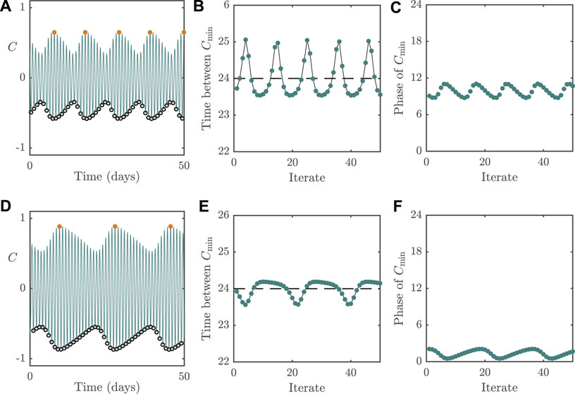
FIGURE 6. Dynamics of the 2D model with $I=1000$ at ${\tau }_c$ values just beyond the Neimark–Sacker bifurcation points with ${\tau }_c=21.8$$<{\tau }_c^{\text{N}1}$ [panels (A–C)] and ${\tau }_c=26.1$$>{\tau }_c^{\text{N}2}$ [panels (D–F)]. (A) + (D): Trajectories of C highlighting modulation in the amplitude of the circadian oscillations. Open black circles indicate the daily $C_{\text{min}}$ values, and solid orange circles indicate the peak values of C for the longer time scale amplitude modulation which has a period of $\sim$11 days in panel (A) and $\sim$18 days in panel (D). The remaining panels are organised in the same manner as in Figure 5.

For parameter values near the Neimark–Sacker instabilities, we see that the cycle-to-cycle period of C now varies around 24 h, as can be seen in Figures 6B,E. The consequence of this is that the phase of C relative to the external forcing, although varying from cycle-to-cycle, is constrained to an interval around the correct phase (i.e., the phase of the underlying limit cycle), as shown in Figures 6C,F. This means that even though people with such dynamics will not be entrained to a 24 h period, their phase variation relative to the external forcing will be of small amplitude, meaning that they may not experience significant circadian rhythm disorders. Overall, this highlights the importance of high light intensities (or, equivalently, in boosting sensitivity to light) for combating non-24 h sleep/wake disorders.

3.5 Summary of Bifurcation Analysis

The observations of the one-parameter continuations may be summarised via the three-parameter bifurcation diagram as shown in Figure 7A, with two-dimensional slices of the full diagram shown in Figures 7B–D. Figure 7A shows the surfaces of fold bifurcations (purple) together with the surfaces of Neimark–Sacker bifurcations (teal) that bound parameter regimes (indicated in Figures 7B–D) with different entrainment behavior. Figure 7B and Figure 7C showcase the so-called Arnol’d tongues that are commonly observed in forced oscillator systems. In the central, light orange shaded, region in Figure 7B, bounded by the Neimark–Sacker (teal) and fold (purple) bifurcation lines, only the stable periodic orbit exists and so the system entrains easily. In the lower, darker orange shaded part of the central region, the stable, unstable and saddle periodic orbits coexist. In this region, the system ultimately converges to the stable periodic orbit, since it is the only attracting set, but the pathway involved in this convergence may be heavily shaped by the other orbits, as will be investigated in Section 4. In the white region to the left and right of the shaded regions, no stable 24 h period orbit exists and so we conclude that the circadian oscillator does not entrain to a 24 h rhythm. Similarly, the light orange shaded region in Figure 7C supports only a single, stable periodic orbit, whilst the region bounded between the two fold curves possesses all three types of periodic orbit. To the left and right of the outer fold curve, only the unstable orbit exists, and hence there is no possibility to entrain to a 24 h rhythm. Figure 7D shows the so-called Arnol’d onion [25, 28], where we now identify a central portion in which only the stable periodic orbit exists. This is surrounded by a region supporting all three orbit types, which itself is surrounded by the white region with only the unstable orbit.

FIGURE 7

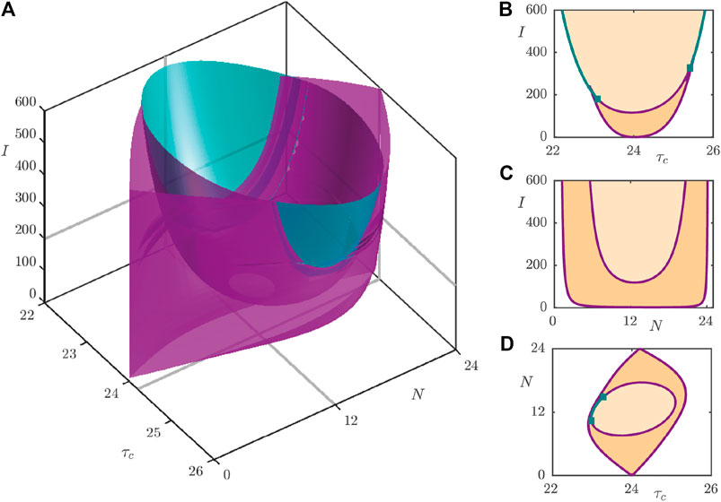
FIGURE 7. (A): Three-parameter bifurcation diagram of the 2D model under variation of $\left(I,N,{\tau }_c\right)$. (B–D): Two-parameter bifurcation diagrams under variation of ($I,{\tau }_c$) for $N=12$ [panel (B)]; ($I,N$) for ${\tau }_c=24.2$ [panel (C)]; and ($N,{\tau }_c$) for $I=200$ [panel (D)]. In all panels, purple lines/surfaces correspond to fold bifurcations, whereas teal lines/surfaces show Neimark–Sacker bifurcations. The square markers in panels (B) and (D) indicate the points at which the Neimark–Sacker and fold curves meet. In the orange shaded regions of panels (B–D) the stable, unstable and saddle periodic orbits exist; in the light orange shaded region only the stable periodic orbit exists. In the surrounding area (white), only the unstable periodic orbit exists and there is no entrainment to a 24 h cycle.

4 Entrainment Times

The bifurcation diagrams in Section 3 indicate where in parameter space the circadian oscillator can be entrained to a 24 h cycle under our choice of forcing. Even in these regions of parameter space, however, the dynamics involved with the entrainment can be markedly different depending on initial conditions. To demonstrate this point, we compute the time taken for a trajectory starting from an arbitrary initial condition to converge to the stable limit cycle; we refer to such times as entrainment times. Formally, we define the entrainment time, $\mathcal{T}\left(X\right)\in {\mathrm{ℝ}}_{\ge 0}$, of an initial condition $X=\left(A,C\right)$ to be

$\mathcal{T}\left(X\right)=\min \left\{t\ge 0|{\Vert {\Phi }_t\left(X\right)-{\Gamma }^s\left(t\right)\Vert }^2\le \epsilon \right\},(9)$

where ε is a tolerance which we hereon set to $\epsilon =0.001$, and ${\text{Γ}}^s$ is the stable limit cycle, defined by

${\text{Γ}}^s\left(t\right)={\text{Φ}}_t\left(X_{\text{L}}^s\right),0\le t<24,(10)$

where $X_{\text{L}}^s$ is the point along the stable limit cycle when $f\left(t\right)$ switches from 0 to 1 (dawn), we refer to this point as the point of zero phase. We denote phase differences along the limit cycle with respect to the point of zero phase by Z, which is defined modulo 24 h.

In Figures 2A,B, we recapitulated results from [25] by plotting the entrainment times for initial conditions along the stable limit cycle at different relative phases (note that the definition of entrainment times between the two studies are different). This section is dedicated to understanding this phenomenon. To this end, we consider a stroboscopic map $P:{\mathrm{ℝ}}^2\to {\mathrm{ℝ}}^2$ defined by

$X_{n+1}=P\left(X_n\right)={\text{Φ}}_{24}\left(X_n\right)={\text{Φ}}_{24-N}^{\text{D}}\circ {\text{Φ}}_N^{\text{L}}\left(X_n\right).(11)$

The above may equivalently be thought of as a Poincaré return map, with a section chosen at the zero phase of the forcing cycle. In Figure 8, we show sequences of map iterates of Eq. 11 for $I=50$ (Figure 8A and Figure 8C) and $I=1000$ (Figure 8E) following an abrupt phase advance of the light/dark cycle, such as that which occurs for positive phase shifts $+\text{Δ}{t}_{\text{s}}$. Figures 8B,D,F show the evolution of the phase of the $C_{\text{min}}$ values relative to the forcing phase. The initial conditions on ${\text{Γ}}^s$ for the Figure 8A and Figure 8C are slightly phase-shifted with respect to each other. The effect of this small difference is evident from the resulting dynamics. In Figure 8A, the iterates move around the orbit in an anti-clockwise fashion, whilst in Figure 8C the iterates follow a clockwise motion. Anti-clockwise iterates correspond to re-entrainment in an orthodromic fashion (i.e., in the same direction as the phase shift of the light/dark cycle) through repetitive phase advancements, as shown in Figure 8B. Conversely, clockwise iterates reflect antidromic re-entrainment (i.e., in the opposite direction as the phase shift of the light/dark cycle) via successive phase delays, as shown in Figure 8D. The sensitivity around the initial conditions in Figure 8A and Figure 8C suggests the presence of a “neutral point” at which the behaviour switches from anti- to orthodromic re-entrainment.

FIGURE 8

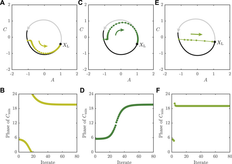
FIGURE 8. Long re-entrainment times for $I=50$ through phase-advancement [panels (A) + (B)] or phase-delay [panels (C) + (D)]. (E) + (F): Fast re-entrainment for $I=1000$, whereby a trajectory takes a “shortcut” instead of advancing or delaying. Note the panel labelling is now column-wise. Panels (A, C, E) show the stable limit cycle for the relevant value of I, the grey arrow indicates the direction of the phase shift of the light/dark cycle. The point of zero phase $X_{\text{L}}$ along the orbits is marked by a black circle. The coloured arrows indicated the direction the iterates move around the orbit. Panels (B, D, F) show the evolution of the phase of the $C_{\text{min}}$ values relative to the forcing phase.

In Figure 8E, we plot iterates for the map with $I=1000$ with an initial condition close to the neutral point. Rather than displaying anti- or orthodromic behaviour, the sequence of iterates cuts directly across the phase space, appearing to take a “shortcut”, rather than re-entraining via gradual phase advancement or delay. This shortcut-type behaviour is reflected by the decrease in entrainment time observed at a phase shift of $\text{Δ}{t}_{\text{s}}\approx +10$ as shown in Figure 2. In [25], the neutral point appears as an unstable fixed point of a one-dimensional entrainment map whose section was chosen to be transverse to the stable limit cycle at the point of zero phase. Here, we will show that the neutral point can be understood by examining (strong) stable manifolds of the stable and saddle fixed points of the stroboscopic map.

4.1 Manifolds as Organisers of Entrainment Times

We compute manifolds following the steps outlined in Supplementary Material S2. Figure 9 shows the projection of the periodic orbits in the $\left(A,C\right)$-plane with the fixed points of Eq. 11 indicated with a marker, and the corresponding stable and unstable manifolds of the points for $I=50$ and $I=1000$. In Figure 9A, we plot the manifolds of the three fixed points (corresponding to stable, saddle, and unstable limit cycles of the 2D model) for $I=50$. The stable manifolds (blue lines) of the stable and saddle fixed points are approximately linear for this parameter set, whilst the unstable manifolds (red lines) of the saddle and unstable fixed points curve away from the fixed points, following the periodic orbits more closely. If we focus specifically on the manifolds associated with the saddle orbit, we can clearly see how the manifolds organise the behaviour observed in Figures 8A–D. In particular, the orthodromic and antidromic re-entrainment behaviour closely follow the trajectory charted by the unstable manifold of the saddle point. The separatrix is given by the stable manifold of the saddle point $X_{\text{L}}^{\text{saddle}}$, and the neutral point is the intersection of the same stable manifold with the projection of the periodic orbit onto the plane of zero phase. Importantly, we have that $\left|{\lambda }_{\text{saddle}}^{\text{s}}-1\right|>\left|{\lambda }_{\text{saddle}}^{\text{u}}-1\right|$ so that contraction toward $X_{\text{L}}^{\text{saddle}}$ along the stable manifold is stronger than repulsion away from the same point along its unstable manifold. This means that trajectories near $X_{\text{L}}^{\text{saddle}}$ get pulled toward the saddle limit cycle before slowing moving away, explaining the long entrainment times near this point in the simulations shown in Figure 2. This observation is confirmed by examining entrainment times for initial conditions across a range of $\left(A,C\right)$ values, as shown in Figure 9B, which we compute according to Eq. 9via simulation over a GPU architecture. Superimposed on these entrainment time heat maps are the stable manifold of the saddle limit cycle and strong stable manifold of the stable limit cycle. In this figure, we see that peaks in the entrainment times occur exactly along the stable manifold of the saddle. If we examine the unstable manifolds of the saddle point in Figure 9A, we see that they organise the orthodromic and antidromic return to the stable fixed point shown in Figures 8A,C. As such, the stable manifold of the saddle point serves as a separatrix between trajectories exhibiting these two kinds of behaviour.

FIGURE 9

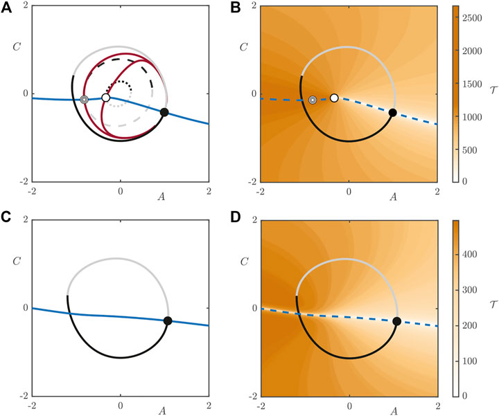
FIGURE 9. Intersections of the manifolds of the periodic orbits of the 2D model with the plane of zero phase for $I=50$ [panels (A) + (B)] and $I=1000$ [panels (C) + (D)]. (A) + (C): Manifolds of the stable and saddle periodic orbits [panel (A)] and of the stable periodic orbit [panel (C)]. Stable and strong stable manifolds are depicted in blue, whilst unstable manifolds are red. Also plotted are the projections onto the plane of zero phase of the stable (solid lines), saddle (dashed lines), and unstable (dotted lines) periodic orbits in black and grey. The markers denote the points of zero phase along the respective periodic orbits. (B) + (D): Heat maps of entrainment times, $\mathcal{T}$, of trajectories with initial conditions distributed across the $\left(A,C\right)$ plane. The dashed blue lines are the strong stable manifolds of the stable periodic orbit [panels (B) + (D)] and the stable manifold of the saddle periodic orbit [panel (B)].

If we increase the light intensity to $I=1000$, the saddle and unstable orbits are no longer present, having disappeared via a fold bifurcation. In this case, we observe that the stable manifolds of the stable limit cycle are responsible for organising behaviour near the neutral point as shown in Figure 9C. Now we can see that the shortcut shown in Figure 8E corresponds to trajectories that follow this stable manifold, which is confirmed in the heat map in Figure 9D.

This plot highlights the existence of a “river” of points in the $\left(A,C\right)$ plane centred on the strong stable manifold of the stable limit cycle that possess significantly lower entrainment times than points around them. We are now in a position to demonstrate how the global maximum at $\text{Δ}{t}_{\text{s}}\approx 10.5$ for $I=50$ becomes a local minimum for $I=1000$. As the fixed points of Eq. 11 corresponding to the fully unstable and saddle fixed points approach each other and coalesce at fold point $I_{\text{F}2}$, the stable manifolds of the saddle and stable limit cycles also approach one other. Since the manifolds vary smoothly with respect to the system parameters, the stable manifold of the saddle limit cycle is effectively replaced by the strong stable manifold of the stable limit cycle as the system moves through the bifurcation. For $I>I_{\text{F}2}$, trajectories close enough to the strong stable manifold of the stable limit cycle can now follow the shortcut, though most trajectories still follow the typical orthodromic and antidromic re-entrainment routes. As I increases, the width of the river increases, so that more trajectories entrain to the limit cycle quickly, though we remark that this width ultimately saturates as I continues to increase.

Thus far, we have set $t_{\text{s}}=0$, setting the point of zero phase to occur exactly at dawn [when $f\left(t\right)$ switches from 0 to 1]. As time zones change, or as a result of changing shift work patterns, the phase of the intrinsic circadian clock will become shifted with respect to the external forcing, causing a shift in $t_{\text{s}}$. Note that variations in $t_{\text{s}}$ do not change the location of limit cycles in the system, rather, they cause the point of zero phase to rotate around the orbit. A similar observation holds for the manifolds. This is demonstrated in Figure 10A, where we plot the stable manifold of the saddle limit cycle and strong stable manifold of the stable limit cycle for $I=50$, shown in Figure 9B, for a sequence of values of $t_{\text{s}}$. In fact, if we denote the set of points comprising a particular manifold in the system with an arbitrary value for $t_{\text{s}}$ at a general forcing phase, θ, by $W_{t_{\text{s}}}^{\theta }$, we have that $W_{t_{\text{s}}}^{\theta }$ is equal to the image under the flow of the system of $W_0^0$ for duration $\theta -t_{\text{s}}$ that is:

$W_{t_{\text{s}}}^{\theta }=\{\begin{array}{cc}{\text{Φ}}_{\theta -t_{\text{s}}}^{\text{L}}\left(W_0^0\right),& 0\le \theta -t_{\text{s}}\le N\\ {\text{Φ}}_{\theta -t_{\text{s}}-N}^{\text{D}}\circ {\text{Φ}}_N^{\text{L}}\left(W_0^0\right),& N<\theta -t_{\text{s}}<24\end{array},(12)$

noting that $\theta -t_{\text{s}}$ should be treated modulo a 24 h period. The natural rotation induced by the flow gives rise to the rotated position of the manifolds as $t_{\text{s}}$ and θ vary. This relationship allows us to trace out the manifolds over the entire forcing cycle, which we display in Figure 10B for the default parameters as listed in Table 1; compare to Figure 3D. The integrated manifolds can then be used to separate trajectories that follow orthodromic vs antidromic re-entrainment for arbitrary phase shifts and at arbitrary phases of the forcing cycle.

FIGURE 10

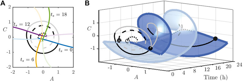
FIGURE 10. (A): Intersection of the strong stable manifolds (dark coloured) of the stable periodic orbit and stable manifolds (light coloured) of the saddle periodic orbit for the indicated values of $t_{\text{s}}$. The projection of each periodic orbit (black and grey) onto this plane of zero phase is also shown. We see that the manifolds rotate around each orbit as $t_{\text{s}}$ is varied, as evidenced by comparing the manifolds with $t_{\text{s}}=0$ and $t_{\text{s}}=12$. (B): Strong stable manifolds of the stable limit cycle (dark blue) and stable manifolds of the saddle limit cycle (light blue) along the entire 24 h forcing cycle.

5 Application to Shift Work

In developed economies, millions of people either permanently work the night shift or rotate in and out of night shift work. When a worker rotates from day shift to night shift, or vice versa, the abrupt change in the pattern of their exposure to light can cause circadian misalignment and jet lag-like symptoms until they entrain to the light/dark cycle of the new shift. Here we study the dynamics of re-entrainment following shift work rotations and use the manifolds of the stable and saddle limit cycles discussed in Section 4.1 to explain the simulation results shown in Figure 2. In particular, we focus on the following two questions. Firstly, at low light intensity ($I=50$), why does it take longer to re-entrain after rotating from night shift to day shift (NS→DS: 1,360 h) than it does after rotating from day shift to night shift (DS→NS: 802 h)? Secondly, why is this asymmetry reversed at higher light intensity ($I=1000$), with a shorter re-entrainment time after rotating from night shift to day shift (NS→DS: 329 h) than after rotating from day shift to night shift (DS→NS: 392 h)?

We assume that a worker on the day shift works from 7 AM to 3 PM and sleeps from 11 PM to 6 AM, whereas someone on the night shift works from 11 PM to 7 AM and sleeps from 8 AM to 3 PM. In either case, they are exposed to $N=17$ hours of light. For both DS and NS workers, “dawn” (i.e., when their light exposure begins) occurs at the $Z=0$ location on the stable limit cycle. Similarly, “dusk” (when their light exposure ends) occurs at the $Z=17$ location for both DS and NS workers. However, DS and NS workers are at these locations on the limit cycle at different wall-clock times: $Z=0$ corresponds to 6 AM for DS workers and 3 PM for NS workers; $Z=17$ corresponds to 11 PM for DS workers and 8 AM for NS workers. With regards to our previous notation, the switch from DS→NS corresponds to $\text{Δ}{t}_s=16$ and the switch from NS→DS represents a value of $\text{Δ}{t}_s=22$.

5.1 Rotating From Day Shift to Night Shift at Low Light Intensity

To simulate a worker rotating from day shift to night shift, we assume that they remain entrained to the DS light/dark cycle until 11 PM, which is the $Z=17$ location indicated by the solid teal dot in Figure 11A. If they were staying on DS, this would be dusk. However, since they are rotating to NS, instead of going to bed they go to work and receive additional light exposure which perturbs them away from the stable limit cycle. More specifically, the DS worker rotating to NS will receive nine extra hours of light before going to bed at 8 AM. This can be thought of as equivalent to traveling nine time zones in the westward direction. By contrast, a worker that is already entrained to the NS light/dark cycle will not be at the $Z=17$ location on the stable limit cycle at 11 PM. Rather, they will be at the $Z=8$ location indicated by the solid orange dot in Figure 11A. The orange periodic orbit shown in Figure 11B represents the entrained NS worker, and the teal trajectory represents the DS worker switching to NS. Re-entrainment is considered complete when the Euclidean norm of the difference between the teal and orange trajectories first falls below the tolerance ε. To help visualise the re-entrainment process, we strobe the system every 24 h and plot the location of the re-entraining trajectory in the $\left(A,C\right)$ plane as open teal dots in Figure 11A and as filled teal dots in the time course shown in Figure 11B. For reference, the strobed iterates of the entrained NS worker are shown as filled orange dots. From Figure 11A, we see that the iterates of the stroboscopic map move along the unstable manifold of the saddle limit cycle until they converge to the location of the entrained NS worker.

FIGURE 11

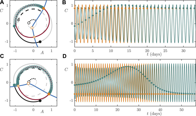
FIGURE 11. Low lux ($I=50$) entrainment dynamics for ${\tau }_c=24.2$ and $N=17$. (A) + (B): Dynamics following transition from day shift to night shift (DS→NS). (A): Projections of the periodic orbits, and their points of zero phase, for the day shift are shown in black (and grey). The points of zero phase corresponding to the periodic orbits for the night shift (which has a different phase of entrainment than the day shift) are shown in orange. The unstable and (strong) stable manifolds of the periodic orbits at the phases indicated by the orange markers are shown in red and blue, respectively. The worker transitions from DS→NS when $f\left(t\right)=1\to f\left(t\right)=0$, with their instantaneous $\left(A,C\right)$ values at this time indicated by the solid teal dot (to the left of the panel). The open teal markers indicate the $\left(A,C\right)$ values of the trajectory starting from this point evaluated at successive 24 h intervals. The trajectory ultimately converges to the entrained phase indicated by the solid orange marker. (B): Time course of C of the entraining trajectory (teal) as it converges to the stable entrained periodic orbit of the night shift (orange). Solid markers on each trajectory indicate the C value of the trajectory evaluated at successive 24 h intervals [corresponding to the open teal markers in panel (A)]. (C) + (D): Dynamics following transition from night shift to day shift (NS→DS), following the same format as panels (A, B). See the Supplementary Material for movies of the entraining trajectories.

5.2 Rotating From Night Shift to Day Shift at Low Light Intensity

Next we consider a worker rotating from night shift to day shift. We assume that they remain entrained to the NS light/dark cycle until 8 AM, which is at the $Z=17$ location on the stable limit cycle indicated by the solid teal dot in Figure 11C. If they were staying on NS, this would be “dusk”. However, since they are rotating to DS, instead of going to bed they remain at work, and receive additional light exposure which perturbs them away from the stable limit cycle. More specifically, the NS worker rotating to DS will receive 15 extra hours of light before going to bed at 11 PM. This can be thought of as equivalent to traveling 9 time zones in the eastward direction. In contrast, a worker that is already entrained to the DS light/dark cycle will not be at the $Z=17$ location on the stable limit cycle at 8 AM. Rather, they will be at the $Z=2$ location indicated by the solid orange dot in Figure 11C. The orange periodic orbit shown in Figure 11D represents the entrained DS worker, and the teal trajectory represents the NS worker rotating to DS. Similarly to the NS→DS scenario described in Section 5.1, in the $\left(A,C\right)$ plane, we see that the iterates of the stroboscopic map move along the unstable manifold of the saddle limit cycle (red curve) until they converge to the location of the entrained DS worker (Figure 11B). However, a key difference between the two scenarios is the location of the stable manifold of the saddle limit cycle. The stable manifold of the saddle limit cycle (blue curve) passes through the projection of the stable limit cycle onto the plane of zero phase (black/grey orbit) near the $Z=17$ location for the NS→DS case, but does not do so for the DS→NS case. In the NS→DS case, the first few iterates move along the stable manifold, passing close to the saddle point of the Poincaré map Eq. 11 before starting to slowly move away from this point along its unstable manifold, leading to the very long re-entrainment time of 57 days shown in Figure 11D. In the DS→NS case, the first few iterates do not move along the stable manifold and thus do not pass as close to the saddle point and therefore move away from the point along its unstable manifold more quickly, leading to the relatively shorter re-entrainment time of 33 days shown in Figure 11B.

5.3 Rotating Between Shifts at High Light Intensity

We assume the same shift work schedules and rotation protocols as in Section 5.1 and 5.2. With $I=1000$, the saddle limit cycle that played such a key role in the behavior for $I=50$ no longer exists. The strong stable manifold of the stable limit cycle passes through the projection of the stable limit cycle onto the plane of zero phase near the $Z=17$ location for NS→DS scenario (Figure 12A), but not for DS→NS scenario (Figure 12C), similarly to the situation with the stable manifold of the saddle limit cycle at low light intensity. In the NS→DS scenario with $I=1000$, the stroboscopic map iterates move along the strong stable manifold, taking the shortcut through phase space and re-entraining in 13.7 days (Figure 12D). In the DS→NS scenario with $I=1000$, the map iterates are not near the strong stable manifold and thus do not have access to the shortcut, leading to a relatively longer re-entrainment time of 16.3 days (Figure 12B). This example highlights the importance of the strong stable manifold of the stable limit cycle in organising re-entrainment dynamics under changes in shift work patterns.

FIGURE 12

FIGURE 12. High lux ($I=1000$) entrainment dynamics for ${\tau }_c=24.2$ and $N=17$. Panel order and format are the same as in Figure 11. (A) + (C): Note here that only the stable periodic orbit exists, and the starting point for the re-entraining trajectory (solid teal dot) in panel (C) is close to the stable manifold (blue curve) that constitutes the “shortcut” to entrainment. See the Supplementary Material for movies of the entraining trajectories.

6 Discussion

The first key result of our paper is the identification of the boundaries of the parameter regimes in which the circadian oscillator can entrain to external forcing. To this end, we perform one-parameter continuation of the periodic orbits in each of light intensity I, day length N and natural period ${\tau }_c$, to identify their codimension-one bifurcations. We then continue these fold and Neimark–Sacker bifurcations in each pair of parameters. This approach leads us to identify Arnol’d tongue structures in the $\left({\tau }_c,I\right)$ and $\left(N,I\right)$ parameter planes. Arnol’d tongues demarcate the region of stability of entrained solutions of systems of forced oscillators, tracing out bifurcations to instability of such solutions [29]. In our study, we not only compute the outer tongue structure of the entrained 24 h solution, but also show how other bifurcations within the tongue change the transient dynamics of trajectories converging to this solution. In the $\left({\tau }_c,N\right)$-plane, we instead find the so called “Arnol’d Onion” shown in Figure 7D in which the widest parameter window for entrainment occurs at $N=12$. The Arnol’d Onion entrainment region was first identified in a generic amplitude-phase-oscillator model of a circadian clock [28]. It has also been found in the $\left(I,{\tau }_c\right)$ and $\left(N,{\tau }_c\right)$-planes via computation of entrainment times in the reduction of the FJK model to a one-dimensional iterative entrainment map [25]. In this paper, using numerical continuation and bifurcation analysis, we identify not only the boundaries of the entrainment region, but also the structure within the area of entrainment. This allows us to distinguish two distinct parameter regimes for entrainment, one where the stable periodic orbit is the only asymptotic solution, and one that contains a saddle periodic orbit, the existence of which leads to longer entrainment times. Via concatenation of two-parameter bifurcation diagrams, we extend the boundaries of all parameter regimes into the full $\left(I,N,{\tau }_c\right)$-space.

Interestingly, Schmal et al. [28] identify higher order “strings” of onions for lower ${\tau }_c$ values, specifically ${\tau }_c=24/K$ where K takes the value of any of the factors of 24, and gives the number of onions (entrainment regions) in the string. In our model, we too identify regions of entrainment for fractional values of the natural period near ${\tau }_c\approx 3.4,4.8$, and 8 which appear as additional branches of solutions that are terminated and initiated via fold bifurcations. These regions are shown in Figure S13 in Supplementary Material S3 for $N=12$ and I = 150, thereby extending Figure 4, along with the associated “strings of onions” in the $\left({\tau }_c,N\right)$-plane. The majority of people have a natural period between 23.5 and 24.7 h so it is unlikely that these branches play a significant role in entrainment dynamics [22]. However, for individuals that do exhibit extremely low ${\tau }_c$ values, these results suggest that entrainment to a 24 h cycle is possible, in spite of the wide discrepancy between the forcing period and their natural period.

The second key result of our paper is the computation of the geometric structures in phase space that organise previously observed re-entrainment dynamics; namely, the invariant manifolds of fixed points for a 24 h stroboscopic map constructed from the model. Computation of these manifolds allows us to find and fully characterise a separatrix between phase advancing and phase delaying re-entrainment trajectories. This phase space separatrix was conjectured to exist following studies of the one-dimensional iterative map reduction of the FJK model [25]. The separatrix is also responsible for the rapid re-entrainment phenomenon that has been observed under certain conditions in simulations and experiments [24, 25, 30–32]. If we interpret Figure 2B as representing entrainment times following international travel, we see that for low light intensity, the longest entrainment times occur for journeys approximately 10 h East ($+10\text{Δ}{t}_{\text{s}}$). This is the East-West jet lag asymmetry phenomenon whereby travelling East results in longer entrainment times and worse reported jet lag [25, 33]. By contrast, for high light intensity, this same figure indicates that this global maximum over entrainment times becomes a local minimum leading to a so-called “shortcut” to entrainment. Diekman and Bose identified this change from a maximum to a minimum in their 1D map and hypothesised that the shortcut corresponds to a phaseless set where isochrons of the periodic orbit converge [25]. Here we show that it is the composition of the separatrix that organises this behaviour. For low light intensity, when the separatrix consists of the strong stable manifold of the stable fixed point and the stable manifold of the saddle point of the stroboscopic map there is a local (in phase space) increase in entrainment times. For high light intensity, the saddle point no longer exists and the separatrix consists of only the strong stable manifold of the stable point enabeling entrainment trajectories that start close to the manifold to exhibit a local decrease in entrainment times.

Invariant manifolds of saddle orbits as organizing centres of entrainment times have recently been identified in a forced Kuramoto model of pacemaker cell dynamics [24] and a hierarchical system of planar Novak–Tyson models [26]. Moreover, the shortcut traced out by the strong stable manifold has recently been experimentally identified from wearable device data and exploited to develop jet lag strategies that align with it [32]. Here, jet lag is measured by self-reported mood scores that show that people who appear to hit the shortcut feel “better” according to a simple positive-negative scale. The authors propose an algorithm based on simulations of the FJK model [13, 17] to create a schedule for optimum re-entrainment that consists of varying periods of light and dark each day. Their strategies rely on knowing the location in phase space of the “optimal solution”, i.e., the strong stable manifold of the entrainment orbit. Their first approach is to identify the optimal solution for phase space corresponding to the situation immediately after arrival. They propose a light/dark schedule to move initial conditions to this optimal solution, but find that the trajectories never reach the optimum and, for some initial conditions, re-entrainment is not achieved. With respect to our formulation, changing the light/dark schedule corresponds to varying the parameter N, which leads to a shift in the position of relevant manifold(s). The authors’ second approach is to update the schedule to fit the optimum for the system at the next step (N value). They show this is a superior strategy in that it leads to faster re-entrainment for all initial conditions. In both cases, the approach to finding the “optimal solution” is a brute force simulation method over the phase space. Here, we directly compute the optimal solution for high light intensity values as the strong stable manifold of the stable fixed point of the stroboscopic map defined by Eq. 11.

Our bifurcation analysis, as presented in Figure 7, shows the boundaries of the entrainment region in the three-parameter space consist of both fold and Neimark–Sacker bifurcations. In particular, Figure 7B suggest that loss of entrainment due to a Neimark–Sacker bifurcation in the $(I,{\tau }_c$)-plane occurs when the light intensity value is high and ${\tau }_c$ is far from 24.2. In Figures 5, 6, we show that the type of bifurcation associated with lack of entrainment has important implications for the resulting dynamics. A ${\tau }_c$ value close to the Neimark–Sacker bifurcation leads to toroidal dynamics in which the phase difference between the circadian oscillator and the external forcing is bounded, whereas a ${\tau }_c$ value close to a fold leads to quasiperiodic dynamics in which this phase discrepancy is constantly slipping. We hypothesise that being close to a fold bifurcation would cause significantly different circadian rhythm disorders compared to being close to a Neimark–Sacker bifurcation. In particular, close to the Neimark–Sacker bifurcation, whilst the circadian rhythm is not entrained to the external environment, the phase difference between the two over successive days is constrained to be within a finite interval. Thus, we expect circadian disorders to be less severe than in the case of the fold bifurcation in which sequential phase differences between the circadian rhythm and the external environment span the entire circle.

Examining the relationships between parameters for light sensitivity G, light intensity scaling factor ${\alpha }_0$ and I in Eq. 4, we observe that a low light intensity is equivalent to when individuals have a low sensitivity to light. We remark here that our BVP set up allows parameters in the model, other than the three presented, to be varied. We would expect that the results when varying G or ${\alpha }_0$ would be similar to those we present for I. It is important to note that the jet lag strategies identified by [32] account for differences in an individual’s intrinsic period (${\tau }_c$). Importantly, they show that personalisation to an individual’s circadian clock improves the effectiveness of the scheduled recovery. Taken together, this suggests that taking into account the interplay between light intensity value (or light sensitivity) and intrinsic rhythm could further improve jet lag strategy development and develop personalised treatment plans for individuals with non-24 h sleep/wake disorder.

Our approach to the set-up of the continuation problem is to establish a multi-segment two-point boundary value problem in Auto [34, 35] to find and follow the periodic orbits of the two-dimensional FJK system. This approach was facilitated by our choice, for simplicity, of a square wave function Eq. 6 for the light/dark forcing giving instantaneous transitions at dawn/dusk. This multi-segment approach is similar in spirit to that taken in [36, 37]. This approach can be readily modified to include, for example, more realistic light protocols, such as variations in the quality and intensity of light similar to those studies in the green unicellular alga Ostreococcus tauri [38, 39]. Here we choose a two-state model that switches from complete darkness to full light, this could readily be extended in future studies to incorporate multiple light levels such as indoor and outdoor light regimes as well as darkness, as used in [40]. Including additional light levels as different “steps” would correspond to having additional segments in our multi-segment BVP with similar matching conditions at the transition times. This multi-segment approach has limitations and an alternative approach would be to convert the 2D autonomous system into a 3D non-autonomous one for implementation in Auto. This alternative approach would allow us to relax the condition on the light/dark forcing and use, for example, a sinusoidal signal reflecting a more gradual change, closer to the real light/dark cycle. Moreover, our choice of multi-segment encoding of the model means that the time shift parameter $t_{\text{s}}$ is not explicitly defined in the BVP, whereas the alternative approach allow $t_{\text{s}}$ to be explicitly specified during continuation runs. We note that to compute the manifolds for specific values of $t_{\text{s}}$ as displayed in Figures 10–12, we make use of the relationship defined in Eq. 12.

The framework we propose here can in principle be extended to the analysis of arbitrary perturbations by computing the invariant manifolds and periodic orbits that constitute organising structures of the system. In Figures 11, 12 we compare two such example perturbations in the context of shift work, the change from night to day shift and vice versa. This approach could be used to identify non-pharmacological strategies for shift workers thereby minimising the risk factors for a range of chronic diseases including cancer, metabolic syndrome and stroke [41]. Another interesting problem to consider is to use our approach to design “compromise” schedules for permanent night shift workers that avoid circadian misalignment during the work week yet also enable them to be awake during daylight hours on weekends thereby improving quality of life [42, 43].

Our study centres around a two dimensional reduction of the FJK model. The reduction of the original system to a planar one facilitates the construction of the full invariant manifolds of the system, as depicted in Figure 10B. Such construction was achieved by first computing one dimensional manifolds of an appropriately chosen stroboscopic map and then by taking integrating these manifolds around the entire forcing cycle. Advances in numerical continuation algorithms, such as those included in the recent Matlab-based CoCo package [44], provide functionality to compute two-dimensional manifolds directly, so that our approach could then be used to compute manifolds for the original three-variable FJK model (though we remark that visualising manifolds of systems with more than two dimensions is difficult). Given the significant similarity between the original FJK model and our 2D variant, we expect that similar conclusions about the role of invariant manifolds in organising re-entrainment dynamics would be observed in the full FJK model.

In addition to the FJK model, there exist a number of other models that describe different aspects of circadian rhythms, such as variability in the expression of clock proteins [45–47], or describe the dynamics of the suprachiasmatic nucleus in a more physiological manner [48]. It remains an open question as to how our results might relate to such models. In this regard, it is worth noting that dynamics in general systems can be at least partially understood via analysis of their invariant sets and associated manifolds. As such, whilst the specific observations we make may not directly carry over to these different models, the general approach is likely to still be valid. Regarding our specific choice of system, we remark the original FJK model was constructed using empirical data from human participants [13, 17]. We believe that this fact coupled with the focus on simple descriptions of core macroscopic variables makes it the ideal model for our study. One important macroscopic variable not included in the FJK model is that of sleep duration. Even in the absence of variation in circadian phase, the dynamics of the sleep/wake cycle are intricate [49]. Given the tight bidirectional coupling between circadian rhythms and sleep/wake cycles, incorporation of sleep as a macroscopic variable promises to be an interesting direction for future investigation [50, 51].

It is well known that seasonality of day length affects the circadian rhythms of humans, animals, and plants [28, 52–54]. More recently, switching between different seasonal day lengths (such as travelling from winter to summer) has been studied by considering the phase response curves of a heuristic phase-amplitude model [55]. Our modelling framework presented here could readily be adapted to identify the organising structures, in particular, the invariant manifolds that organise re-entrainment after sudden seasonal switches. A further model extension, that to our knowledge has not been modelled before, is to incorporate forcing at multiple time scales the encompass both day length and seasonality. Additionally, on even longer timescales, there is evidence from evolutionary biology that human core body temperature is decreasing [56] and it is not clear what effect this will have on circadian rhythms.

7 Conclusion

In this paper, we study the loss of entrainment in a two-dimensional reduction of the forced FJK model for human circadian rhythms. We use bifurcation theory to identify parameter regimes in which the circadian oscillator is unable to entrain to a 24 h cycle and identify the instabilities leading to this phenomenon under variation of key system parameters. For parameter regimes where entrainment is attainable, we show how re-entrainment times are organised by the invariant manifolds of the periodic orbits of the system. Finally, we study re-entrainment following phase shifts of the light/dark cycle and discuss these results in the context of shift work transitions.

Code Availability

AUTO, Python, CUDA, and Matlab code needed to reproduce all results in this manuscript may be downloaded via Git from https://github.com/kyle-wedgwood/EntrainmentTimesManifolds. For help with installing software or running code, please contact k.c.a.wedgwood@exeter.ac.uk.

Data Availability Statement

Publicly available datasets were analyzed in this study. This data can be found here: https://github.com/kyle-wedgwood/EntrainmentTimesManifolds.

Author Contributions

JC, CD, and KW contributed to conception and design of the study. JC performed the continuation in AUTO. CD and KW performed simulations of entrainment times. JC, CD, and KW wrote sections of the manuscript. All authors contributed to manuscript revision, read, and approved the submitted version.

Funding Statement

JC gratefully acknowledges funding from MRC Skills Development Fellowship MR/S019499/1. CD gratefully acknowledges the financial support of the US-UK Fulbright Commission, the EPSRC via grant EP/N014391/1, and the National Science Foundation via grant DMS 1555237. KW gratefully acknowledges the financial support of the EPSRC via grant EP/T017856/1 and from MRC via the Skills Development Fellowship MR/P01478X/1.

Conflict of Interest

The authors declare that the research was conducted in the absence of any commercial or financial relationships that could be construed as a potential conflict of interest.

Publisher’s Note

All claims expressed in this article are solely those of the authors and do not necessarily represent those of their affiliated organizations, or those of the publisher, the editors and the reviewers. Any product that may be evaluated in this article, or claim that may be made by its manufacturer, is not guaranteed or endorsed by the publisher.

Acknowledgments

We would like to thank Peter Ashwin and Amitabha Bose for insightful comments and discussions regarding this project.

Supplementary Material

The Supplementary Material for this article can be found online at: https://www.frontiersin.org/articles/10.3389/fams.2021.703359/full#supplementary-material

Supplementary Video 1 | Movie of the entraining trajectories following rotation from day shift to night shift at (DS→NS) low light intensity I = 50; accompanies Figure 11 A,B. Left panel shows the projections of the periodic orbits, and their points of zero phase, for the day shift in black and grey. The points of zero phase corresponding to the periodic orbits for the night shift (which has a different phase of entrainment than the day shift) are shown in orange. The unstable and (strong) stable manifolds of the periodic orbits at the phases indicated by the orange markers are shown in red and blue, respectively. The worker transitions from day shift to night shift when f(t) = 1 → f(t) = 0, with their instantaneous f(t) = 1 → f(t) = 0, values at this time indicated by the first solid teal dot (to the left of the panel). Subsequent teal markers indicate the f(t) = 1 → f(t) = 0, values of the trajectory starting from this point evaluated at successive 24 h intervals. The trajectory ultimately converges to the entrained phase indicated by the solid orange marker. The right panel shows the C coordinate of the time course of the entraining trajectory (teal) as it converges to the stable entrained periodic orbit of the night shift (orange). Solid markers on each trajectory indicate the C value of the trajectory evaluated at successive 24 h intervals (corresponding to the teal markers in the projection on the left).

Supplementary Video 2 | Movie of the entraining trajectories following rotation from night shift to day shift (NS→DS) at low light intensity I=50; accompanies Figure 11 C,D. Left panel shows the projections of the periodic orbits, and their points of zero phase, for the night shift in black and grey. The points of zero phase corresponding to the periodic orbits for the day shift (which has a different phase of entrainment than the night shift) are shown in orange. The unstable and (strong) stable manifolds of the periodic orbits at the phases indicated by the orange markers are shown in red and blue, respectively. The worker transitions from night shift to day shift when f(t) = 1 → f(t) = 0, with their instantaneous (A,C) values at this time indicated by the first solid teal dot (to the left of the panel). Subsequent teal markers indicate the (A,C) values of the trajectory starting from this point evaluated at successive 24 h intervals. The trajectory ultimately converges to the entrained phase indicated by the solid orange marker. The right panel shows the C coordinate of the time course of the entraining trajectory (teal) as it converges to the stable entrained periodic orbit of the day shift (orange). Solid markers on each trajectory indicate the C value of the trajectory evaluated at successive 24 h intervals (corresponding to the teal markers in the projection on the left).

Supplementary Video 3 | Movie of the entraining trajectories following rotation from day shift to night shift (DS→NS) at high light intensity I=1000; accompanies Figure 12 A,B. Left panel shows the projections of the periodic orbits, and their points of zero phase, for the day shift in black and grey. The points of zero phase corresponding to the periodic orbits for the night shift (which has a different phase of entrainment than the day shift) are shown in orange. The stable manifold of the periodic orbit at the phase indicated by the orange marker is shown in blue. The worker transitions from day shift to night shift when f(t) = 1 → f(t) = 0, with their instantaneous (A,C) values at this time indicated by the first solid teal dot (to the left of the panel). Subsequent teal markers indicate the (A,C) values of the trajectory starting from this point evaluated at successive 24 h intervals. The trajectory ultimately converges to the entrained phase indicated by the solid orange marker. The right panel shows the C coordinate of the time course of the entraining trajectory (teal) as it converges to the stable entrained periodic orbit of the night shift (orange). Solid markers on each trajectory indicate the C value of the trajectory evaluated at successive 24 h intervals (corresponding to the teal markers in the projection on the left).

Supplementary Video 4 | Movie of the entraining trajectories following rotation from night shift to day shift (NS→DS) at high light intensity I=1000; accompanies Figure 12 C,D. Left panel shows the projections of the periodic orbits, and their points of zero phase, for the night shift in black and grey. The points of zero phase corresponding to the periodic orbits for the day shift (which has a different phase of entrainment than the night shift) are shown in orange. The stable manifold of the periodic orbit at the phase indicated by the orange marker is shown in blue, respectively. The worker transitions from night shift to day shift when f(t) = 1 → f(t) = 0, with their instantaneous (A,C) values at this time indicated by the first solid teal dot (to the left of the panel). Subsequent teal markers indicate the (A,C) values of the trajectory starting from this point evaluated at successive 24 h intervals. The trajectory ultimately converges to the entrained phase indicated by the solid orange marker. The right panel shows the C coordinate of the time course of the entraining trajectory (teal) as it converges to the stable entrained periodic orbit of the day shift (orange). Solid markers on each trajectory indicate the C value of the trajectory evaluated at successive 24 h intervals (corresponding to the teal markers in the projection on the left).

References

1. Figueiro, M. Delayed Sleep Phase Disorder: Clinical Perspective with a Focus on Light Therapy. Nat Sci Sleep (2016) 8:91–106. doi:10.2147/nss.s85849

PubMed Abstract | CrossRef Full Text | Google Scholar

2. Emens, JS, and Eastman, CI. Diagnosis and Treatment of Non-24-h Sleep-Wake Disorder in the Blind. Drugs (2017) 77(6):637–50. doi:10.1007/s40265-017-0707-3

PubMed Abstract | CrossRef Full Text | Google Scholar

3. McArthur, AJ, Lewy, AJ, and Sack, RL. Non-24-hour Sleep-Wake Syndrome in a Sighted Man: Circadian Rhythm Studies and Efficacy of Melatonin Treatment. Sleep (1996) 19(7):544–53. doi:10.1093/sleep/19.7.544

PubMed Abstract | CrossRef Full Text | Google Scholar

4. Watanabe, T, Kajimura, N, Kato, M, Sekimoto, M, Hori, T, and Takahashi, K. Case of a Non‐24 H Sleep-Wake Syndrome Patient Improved by Phototherapy. Psychiatry Clin Neurosciences (2000) 54(3):369–70. doi:10.1046/j.1440-1819.2000.00719.x

CrossRef Full Text | Google Scholar

5. Burgess, HJ, and Emens, JS. Circadian-Based Therapies for Circadian Rhythm Sleep-Wake Disorders. Curr Sleep Med Rep (2016) 2(3):158–65. doi:10.1007/s40675-016-0052-1

PubMed Abstract | CrossRef Full Text | Google Scholar

6. Smith, MR, and Eastman, CI. Shift Work: Health, Performance and Safety Problems, Traditional Countermeasures, and Innovative Management Strategies to Reduce Circadian Misalignment. Nat Sci Sleep (2012) 4:111–32. doi:10.2147/NSS.S10372

PubMed Abstract | CrossRef Full Text | Google Scholar

7. Smith, MR, Fogg, LF, and Eastman, CI. A Compromise Circadian Phase Position for Permanent Night Work Improves Mood, Fatigue, and Performance. Sleep (2009) 32(11):1481–9. doi:10.1093/sleep/32.11.1481

PubMed Abstract | CrossRef Full Text | Google Scholar

8. Gonze, D. Modeling Circadian Clocks: From Equations to Oscillations. Cent Eur J Biol (2011) 6(5):699–711. doi:10.2478/s11535-011-0061-5

CrossRef Full Text | Google Scholar

9. Goldbeter, A, and Leloup, J-C. From Circadian Clock Mechanism to Sleep Disorders and Jet Lag: Insights from a Computational Approach. Biochem Pharmacol (2021)(December 2020) 114482. doi:10.1016/j.bcp.2021.114482

PubMed Abstract | CrossRef Full Text | Google Scholar

10. Henson, MA. Multicellular Models of Intercellular Synchronization in Circadian Neural Networks. Chaos, Solitons & Fractals (2013) 50:48–64. doi:10.1016/j.chaos.2012.11.008

CrossRef Full Text | Google Scholar

11. Belle, MDC, and Diekman, CO. Neuronal Oscillations on an Ultra‐slow Timescale: Daily Rhythms in Electrical Activity and Gene Expression in the Mammalian Master Circadian Clockwork. Eur J Neurosci (2018) 48:2696–717. doi:10.1111/ejn.13856

PubMed Abstract | CrossRef Full Text | Google Scholar

12. Asgari-Targhi, A, and Klerman, EB. Mathematical Modeling of Circadian Rhythms. Wiley Interdiscip Rev Syst Biol Med (2019) 11(2):e1439–34. doi:10.1002/wsbm.1439

PubMed Abstract | CrossRef Full Text | Google Scholar

13. Forger, DB, Jewett, ME, and Kronauer, RE. A Simpler Model of the Human Circadian Pacemaker. J Biol Rhythms (1999) 14(6):533–8. doi:10.1177/074873099129000867

CrossRef Full Text | Google Scholar

14. Stone, JE, Postnova, S, Sletten, TL, Rajaratnam, SMW, and Phillips, AJK. Computational Approaches for Individual Circadian Phase Prediction in Field Settings. Curr Opin Syst Biol (2020) 22(August):39–51. doi:10.1016/j.coisb.2020.07.011

CrossRef Full Text | Google Scholar

15. Kronauer, RE. A Quantitative Model for the Effects of Light on the Amplitude and Phase of the Deep Circadian Pacemaker, Based on Human Data. In: J Horne, editor. Sleep ’90, Proceedings of the Tenth European Congress on Sleep Research. Bochum: Pontenagel Press (1990). p. 306–9.

Google Scholar

16. Jewett, ME, and Kronauer, RE. Refinement of Limit Cycle Oscillator Model of the Effects of Light on the Human Circadian Pacemaker. J Theor Biol (1998) 192(4):455–65. doi:10.1006/jtbi.1998.0667

PubMed Abstract | CrossRef Full Text | Google Scholar

17. Jewett, ME, Forger, DB, and Kronauer, RE. Revised Limit Cycle Oscillator Model of Human Circadian Pacemaker. J Biol Rhythms (1999) 14(6):493–500. doi:10.1177/074873049901400608

PubMed Abstract | CrossRef Full Text | Google Scholar

18. Kronauer, RE, Forger, DB, and Jewett, ME. Quantifying Human Circadian Pacemaker Response to Brief, Extended, and Repeated Light Stimuli over the Phototopic Range. J Biol Rhythms (1999) 14(6):500–15. doi:10.1177/074873099129001073

PubMed Abstract | CrossRef Full Text | Google Scholar

19. Indic, P, Forger, DB, Hilaire, MAS, Dean, DA, Brown, EN, Kronauer, RE, et al. Comparison of Amplitude Recovery Dynamics of Two Limit Cycle Oscillator Models of the Human Circadian Pacemaker. Chronobiology Int (2005) 22(4):613–29. doi:10.1080/07420520500180371 Available from: http://www.pubmedcentral.nih.gov/articlerender.fcgi?artid=3797655{\&}tool=pmcentrez{\&}rendertype=abstract.

CrossRef Full Text | Google Scholar

20. St. Hilaire, MA, Klerman, EB, Khalsa, SBS, Wright, KP, Czeisler, CA, and Kronauer, RE. Addition of a Non-photic Component to a Light-Based Mathematical Model of the Human Circadian Pacemaker. J Theor Biol (2007) 247(4):583–99. doi:10.1016/j.jtbi.2007.04.001

PubMed Abstract | CrossRef Full Text | Google Scholar

21. Klerman, EB, and Hilaire, MS. Review: On Mathematical Modeling of Circadian Rhythms, Performance, and Alertness. J Biol Rhythms (2007) 22(2):91–102. doi:10.1177/0748730407299200

PubMed Abstract | CrossRef Full Text | Google Scholar

22. Stone, JE, McGlashan, EM, Quin, N, Skinner, K, Stephenson, JJ, Cain, SW, et al. The Role of Light Sensitivity and Intrinsic Circadian Period in Predicting Individual Circadian Timing. J Biol Rhythms (2020) 35(6):628–40. doi:10.1177/0748730420962598

PubMed Abstract | CrossRef Full Text | Google Scholar

23. Leloup, J-C, and Goldbeter, A. Critical Phase Shifts Slow Down Circadian Clock Recovery: Implications for Jet Lag. J Theor Biol (2013) 333:47–57. doi:10.1016/j.jtbi.2013.04.039

PubMed Abstract | CrossRef Full Text | Google Scholar

24. Lu, Z, Klein-Cardeña, K, Lee, S, Antonsen, TM, Girvan, M, and Ott, E. Resynchronization of Circadian Oscillators and the East-West Asymmetry of Jet-Lag. Chaos (2016) 26(9):094811. doi:10.1063/1.4954275

PubMed Abstract | CrossRef Full Text | Google Scholar

25. Diekman, CO, and Bose, A. Reentrainment of the Circadian Pacemaker during Jet Lag: East-West Asymmetry and the Effects of north-south Travel. J Theor Biol (2018) 437:261–85. doi:10.1016/j.jtbi.2017.10.002

PubMed Abstract | CrossRef Full Text | Google Scholar

26. Liao, G, Diekman, C, and Bose, A. Entrainment Dynamics of Forced Hierarchical Circadian Systems Revealed by 2-dimensional Maps. SIAM J Appl Dyn Syst (2020) 19(3):2135–61. doi:10.1137/19m1307676

CrossRef Full Text | Google Scholar

27. Bordyugov, G, Abraham, U, Granada, A, Rose, P, Imkeller, K, Kramer, A, et al. Tuning the Phase of Circadian Entrainment. J R Soc Interf (2015) 12(108):20150282. doi:10.1098/rsif.2015.0282

PubMed Abstract | CrossRef Full Text | Google Scholar

28. Schmal, C, Myung, J, Herzel, H, and Bordyugov, G. A Theoretical Study on Seasonality. Front Neurol (2015) 6(MAY):94–11. doi:10.3389/fneur.2015.00094

PubMed Abstract | CrossRef Full Text | Google Scholar

29. Glass, L, Guevara, MR, Shrier, A, and Perez, R. Bifurcation and Chaos in a Periodically Stimulated Cardiac Oscillator. Physica D: Nonlinear Phenomena (1983) 7:89–101. doi:10.1016/0167-2789(83)90119-7

CrossRef Full Text | Google Scholar

30. Win free, AT. Resetting the Human Clock. Nature (1991) 350(6313):18. doi:10.1038/350018a0

PubMed Abstract | CrossRef Full Text | Google Scholar

31. Serkh, K, and Forger, DB. Optimal Schedules of Light Exposure for Rapidly Correcting Circadian Misalignment. Plos Comput Biol (2014) 10(4):e1003523. doi:10.1371/journal.pcbi.1003523

PubMed Abstract | CrossRef Full Text | Google Scholar

32. Christensen, S, Huang, Y, Walch, OJ, and Forger, DB. Optimal Adjustment of the Human Circadian Clock in the Real World. Plos Comput Biol (2020) 16(12):e1008445. doi:10.1371/journal.pcbi.1008445

PubMed Abstract | CrossRef Full Text | Google Scholar

33. Taylor, SR. Delays Are Self-Enhancing: An Explanation of the East-West Asymmetry in Recovery from Jetlag. J Biol Rhythms (2021) 36:127–36. doi:10.1177/0748730421990482

PubMed Abstract | CrossRef Full Text | Google Scholar

34. Doedel, EJ. AUTO: A Program for the Automatic Bifurcation Analysis of Autonomous Systems. Congr Numer (1981) 30(265-284):25–93.

Google Scholar

35. Doedel, EJ, Champneys, AR, Dercole, F, Fairgrieve, TF, Kuznetsov, YA, Oldeman, B, et al. AUTO-07P: Continuation and Bifurcation Software for Ordinary Differential Equations (2007). Available from: http://cmvl.cs.concordia.␣ca/auto/.

36. Creaser, Jennifer L., Krauskopf, B, and Osinga, HM. Finding First Foliation Tangencies in the Lorenz System. SIAM J Appl Dyn Syst (2017) 16(4):2127–64. doi:10.1137/17m1112716

CrossRef Full Text | Google Scholar

37. Langfield, P, Krauskopf, B, and Osinga, HM. Solving Winfree's Puzzle: The Isochrons in the FitzHugh-Nagumo Model. Chaos (2014) 24(1):013131. doi:10.1063/1.4867877

PubMed Abstract | CrossRef Full Text | Google Scholar

38. Thommen, Q, Pfeuty, B, Morant, PE, Corellou, F, Bouget, FY, and Lefranc, M. Robustness of Circadian Clocks to Daylight Fluctuations: Hints from the Picoeucaryote Ostreococcus Tauri. Plos Comput Biol (2010) 6(11):e1000990. doi:10.1371/journal.pcbi.1000990

PubMed Abstract | CrossRef Full Text | Google Scholar

39. Thommen, Q, Pfeuty, B, Schatt, P, Bijoux, A, Bouget, FY, and Lefranc, M. Probing Entrainment of Ostreococcus Tauri Circadian Clock by Blue and green Light through a Mathematical Modeling Approach. Front Genet (2015) 5(FEB):1–13. doi:10.3389/fgene.2015.00065

Google Scholar

40. Skeldon, AC, Phillips, AJ, and Dijk, DJ. The Effects of Self-Selected Light-Dark Cycles and Social Constraints on Human Sleep and Circadian Timing: a Modeling Approach. Sci Rep (2017) 7(February):45158. doi:10.1038/srep45158 Available from: http://www.nature.com/articles/srep45158.

PubMed Abstract | CrossRef Full Text | Google Scholar

41. Crowther, ME, Ferguson, SA, Vincent, GE, and Reynolds, AC. Non-Pharmacological Interventions to Improve Chronic Disease Risk Factors and Sleep in Shift Workers: A Systematic Review and Meta-Analysis. Clocks & Sleep (2021) 3(1):132–78. doi:10.3390/clockssleep3010009

CrossRef Full Text | Google Scholar

42. Lee, C, Smith, MR, and Eastman, CI. A Compromise Phase Position for Permanent Night Shift Workers: Circadian Phase after Two Night Shifts with Scheduled Sleep and Light/dark Exposure. Chronobiology Int (2006) 23(4):859–75. doi:10.1080/07420520600827160

CrossRef Full Text | Google Scholar

43. Brum, MCB, Dantas Filho, FF, Schnorr, CC, Bertoletti, OA, Bottega, GB, and da Costa Rodrigues, T. Night Shift Work, Short Sleep and Obesity. Diabetol Metab Syndr (2020) 12(1):13. doi:10.1186/s13098-020-0524-9

PubMed Abstract | CrossRef Full Text | Google Scholar

44. Dankowicz, H, and Schilder, F. Recipes for Continuation. Philadelphia: SIAM (2013).

45. Ruoff, P, Vinsjevik, M, Monnerjahn, C, and Rensing, L. The Goodwin Oscillator: On the Importance of Degradation Reactions in the Circadian Clock. J Biol Rhythms (1999) 14(6):469–79. doi:10.1177/074873099129001037

PubMed Abstract | CrossRef Full Text | Google Scholar

46. Vasalou, C, Herzog, ED, and Henson, MA. Small-World Network Models of Intercellular Coupling Predict Enhanced Synchronization in the Suprachiasmatic Nucleus. J Biol Rhythms (2009) 24(1):243–54. doi:10.1177/0748730409333220 Available from: https://www.ncbi.nlm.nih.gov/pmc/articles/PMC3624763/pdf/nihms412728.pdf.

PubMed Abstract | CrossRef Full Text | Google Scholar

47. François, P, Despierre, N, and Siggia, ED. Adaptive Temperature Compensation in Circadian Oscillations. Plos Comput Biol (2012) 8(7):e1002585–12. doi:10.1371/journal.pcbi.1002585

PubMed Abstract | CrossRef Full Text | Google Scholar

48. Diekman, CO, and Forger, DB. Clustering Predicted by an Electrophysiological Model of the Suprachiasmatic Nucleus. J Biol Rhythms (2009) 24(4):322–33. doi:10.1177/0748730409337601

PubMed Abstract | CrossRef Full Text | Google Scholar

49. Skeldon, AC, Dijk, DJ, and Derks, G. Mathematical Models for Sleep-Wake Dynamics: Comparison of the Two-Process Model and a Mutual Inhibition Neuronal Model. PLoS ONE (2014) 9(8):e103877. doi:10.1371/journal.pone.0103877

PubMed Abstract | CrossRef Full Text | Google Scholar

50. Watson, LA, McGlashan, EM, Hosken, IT, Anderson, C, Phillips, AJK, and Cain, SW. Sleep and Circadian Instability in Delayed Sleep-Wake Phase Disorder. J Clin Sleep Med (2020) 16(9):1431–6. doi:10.5664/jcsm.8516

PubMed Abstract | CrossRef Full Text | Google Scholar

51. Murray, JM, Magee, M, Sletten, TL, Gordon, C, Lovato, N, Ambani, K, et al. Light-based Methods for Predicting Circadian Phase in Delayed Sleep-Wake Phase Disorder. Sci Rep (2021) 11(1):1–12. doi:10.1038/s41598-021-89924-8

PubMed Abstract | CrossRef Full Text | Google Scholar

52. Pittendrigh, CS, and Daan, S. A Functional Analysis of Circadian Pacemakers in Nocturnal Rodents. J Comp Physiol (1976) 106(3):291–331. doi:10.1007/bf01417859

CrossRef Full Text | Google Scholar

53. Hazlerigg, DG, and Wagner, GC. Seasonal Photoperiodism in Vertebrates: from Coincidence to Amplitude. Trends Endocrinol Metab (2006) 17(3):83–91. doi:10.1016/j.tem.2006.02.004

PubMed Abstract | CrossRef Full Text | Google Scholar

54. De Caluwé, J, de Melo, JRF, Tosenberger, A, Hermans, C, Verbruggen, N, Leloup, J-C, et al. Modeling the Photoperiodic Entrainment of the Plant Circadian Clock. J Theor Biol (2017) 420(January):220–31. doi:10.1016/j.jtbi.2017.03.005

PubMed Abstract | CrossRef Full Text | Google Scholar

55. Tokuda, IT, Schmal, C, Ananthasubramaniam, B, and Herzel, H. Conceptual Models of Entrainment, Jet Lag, and Seasonality. Front Physiol (2020) 11:334. doi:10.3389/fphys.2020.00334

PubMed Abstract | CrossRef Full Text | Google Scholar

56. Protsiv, M, Ley, C, Lankester, J, Hastie, T, and Parsonnet, J. Decreasing Human Body Temperature in the United States since the Industrial Revolution. eLife (2020) 9:e49555. doi:10.7554/eLife.49555

PubMed Abstract | CrossRef Full Text | Google Scholar

57. Krauskopf, B, and Osinga, HM. Computing Invariant Manifolds via the Continuation of Orbit Segments. In: Numerical Continuation Methods for Dynamical Systems. Springer (2007). p. 117–54. doi:10.1007/978-1-4020-6356-5_4

CrossRef Full Text | Google Scholar

58. Kuznetsov, YA. Elements of Applied Bifurcation Theory. 2nd ed. Springer-Verlag (1998).

59. England, JP, Krauskopf, B, and Osinga, HM. Computing One-Dimensional Global Manifolds of Poincaré Maps by Continuation. SIAM J Appl Dyn Syst (2005) 4(4):1008–41. doi:10.1137/05062408x

CrossRef Full Text | Google Scholar