Effect of Dichotomization on the Latent Structure of Data

Introduction

Data investigated in empirical research are the outcome of measuring attributes. We follow [1] in perceiving measurement as the mapping of an attribute to a numeric scale. Various tools are used for accomplishing the mapping, as for example observers, questionnaires, tests and apparatuses providing reaction times, EEG recordings and more. The tools differ according to the information that is made available. Because of differences regarding the quality of the provided information, it has become customary to distinguish between different levels of measurement: the nominal, ordinal, interval and ratio levels [2]. Furthermore, there are special levels like the level characterizing dichotomous data. Dichotomous data can be thought of as derived from interval-level data by dichotomization. But interval-level data are continuous and normally distributed [N (μ,σ)] whereas dichotomous data are binary and following a binomial distribution [B (1, p)]. In this paper the following question is addressed: Do dichotomous data show the latent structure of the interval-level data from which they are assumed to originate? This question is of importance because one aim in investigating binary data is achieving information on attributes that are considered as continuous variables following a normal distribution. Furthermore, it is of importance for evaluating the consequences of dichotomization for overcoming distributional problems. This question is addressed in the framework of confirmatory factor analysis.

To illustrate the addressed question we selected four items of a scale measuring personal optimism. These items showed a response format including four ordered categories. We transformed the coded four types of responses of data collected by means of these items into two types by dichotomization. Next, we investigated the structure of the data (N = 209). Fit statistics provided by confirmatory factor analysis signified good model fit (χ² = 2.1, df = 5, RMSEA = 0.0, SRMR = 0.03, CFI = 1.0, NNFI = 1.1). But the factor loadings were only 0.20, 0.19, 0.22 and 0.18 suggesting that the contribution of optimism to responding may be minor. We also investigated the original data. The factor loadings obtained in this investigation (0.64, 0.68, 0.66 and 0.68) suggested a much larger contribution of optimism to responding. It is tempting to blame dichotomization for the apparent change of the latent structure of data.

The Latent Structure

The latent structure of data extends to the dimensionality and amount of systematic variation characterizing data. Regarding the investigation of the effect of dichotomization, the focus is on the amount of systematic variation since a change of dimensionality is unlikely to occur and beyond that can be controlled by investigating model fit.

The amount of systematic variation is reflected by the factor loadings of the model used in data analysis [3]. Factor loadings are constituents of the measurement model of confirmatory factor analysis (CFA) and also of the corresponding covariance matrix (CM) model. The CM model is expected to reproduce the to-be-investigated empirical covariance matrix. The customary versions of CFA and CM models include one latent variable and decomposes manifest variance into systematic and error components [4, 5].

Let ξ be the latent variable with E(ξ) = 0 and Var(ξ) = σ, ξ ∼ N (0, σ), and X₁, … , X_p a set of random variables following a normal distribution. CFA models with one latent variable include ξ for capturing the systematic variation characterizing the set of random variables. In order to assure that systematic variation is represented by σ, some transformations of the CM model are necessary that are described in the following paragraphs.

The CM model of the p × p covariance matrix, ${\displaystyle \sum \left({\displaystyle \sum \in {\Re }^{p\times p}}\right)}$, is defined as

$\Sigma =\lambda \phi \lambda \prime +\theta (1)$

where λ represents the p × 1 vector of factor loadings, ϕ the variance parameter and θ the p × p diagonal matrix of error variables. In the case of one factor ϕ is a scalar. It is not necessarily equivalent to σ. Instead, systematic variation of data is represented by the product of ϕ and λ (and its transpose) whereas θ represents variation due to random influences.

A more concise representation of the systematic variation of data characterizes explorative factor analysis. In this case systematic variation of data is represented by the variance of the factor (= latent variable), $v\left(v\in \Re \right)$, that is defined as sum of squared factor loadings λ_i (i = 1, … , p):

$v={\displaystyle \sum _{i=1}^p{\lambda }_i^2}(2)$

Given the same estimation method and underlying structure, the variances of factor (v) and latent variable (σ) can be expected to correspond. The representation of systematic variation according to Eq. 2 can be also realized within Eq. 1 by scaling.

Scaling of the variance parameter of Eq. 1 according to the reference-group method [6, 7] that means setting the variance parameter equal to one (ϕ = 1), assures that only the factor loadings represent the captured systematic variation. In this case the squared factor loadings sum up to provide the variance of the latent variable (= factor) in the following way:

${\displaystyle \sum _{i=1}^p{\lambda }_i^2}=\text{trace}\left(\lambda \lambda \prime \right)=\text{trace}\left(\lambda \varphi \lambda \prime \right).(3)$

There is also the possibility to (re-)scale variance parameter ϕ so that it represents the variance of the latent variable [8]. This is achieved by transforming the originally estimated factor loadings ${\lambda }_i\left(i=1,\dots p\right)$ into adjusted factor loadings ${\lambda }_i^{\ast }\left(i=1,\dots p\right)$ such that

$1={\displaystyle \sum _{i=1}^p{\lambda }_i^{\ast 2}}(4)$

with ${\lambda }_i^{\ast }=c{\lambda }_i\left(c\in {\Re }^{+}\right)$ in the first step. In the second step the free factor loadings of the model are replaced by the estimated factor loadings as fixed values $\left({\lambda }_i^{\ast }\right)$ whereas the otherwise fixed variance parameter is set free for estimation. Finally, ϕ ^∗ is estimated (that replaces ϕ as variance parameter of the model).

For demonstrating that ϕ ^∗ represents the variance of the latent variable, it is assumed that λ^∗ includes all ${\lambda }_i^{\ast }\left(i=1,\dots ,p\right)$ as fixed entries (i.e., λ^∗ = cλ). Starting from Eq. 3, the following sequence of transformations (from the right-hand side to the left-hand side)

$\begin{array}{l}\varphi \ast \times \text{trace}\left({\lambda }^{\ast }{\lambda }^{\ast }\prime \right)=\varphi \times \frac{1}{c^2}\text{trace}\left(c\lambda c\lambda \prime \right)=\varphi \times \text{trace}\left(\lambda \lambda \prime \right)=\text{trace}\left(\lambda \varphi \lambda \prime \right)={\displaystyle \sum _{i=1}^p{\lambda }_i^2}\end{array}(5)$

suggests that

$\varphi \ast ={\displaystyle \sum _{i=1}^p{\lambda }_i^2}(6)$

since according to Eqs. 3, 4 the trace of λ^∗λ^∗′ must be one. Given the described conditions, the systematic variation of data captured by the latent variable of the CFA model is estimated by ϕ ^∗.

The Input to Confirmatory Factor Analysis

The CM model also gives rise to the expectation of specific input to CFA. The input is either an empirical covariance or correlation matrix that is to be reproduced by the model [9]. The more general event is the covariance matrix. In the case of interval-level data the covariance based on product-moments, cov_PM(X,Y), is computed and integrated in the covariance matrix to serves as input:

${\mathrm{cov}}_{\text{PM}}\left(X,Y\right)=\frac{1}{n}{\displaystyle \sum _{i=1}^n\left(x_i-\overline{x}\right)\times \left(y_i-\overline{y}\right)}(7)$

where $X\left(X\in \Re \right)$ and $Y\left(Y\in \Re \right)$ are the normally distributed random variables, x_i and y_i are the x-score and y-score of the ith participant, $\overline{x}\text{and}\overline{y}$ the corresponding means and n the sample size.

Although dichotomous data can be thought of as derived from interval-level data [N (μ,σ)], they are mostly available as binary data [B (1, p)]. For example, the responses to the items of a scale measuring arithmetic reasoning are usually available as correct and incorrect responses although such a complex ability can be assumed to be measurable with interval-level quality. The typical way of assigning numbers to responses (e.g., 0 = incorrect, 1 = correct) does not reflect the interval level. Furthermore, the coding of the responses does neither create the interval-level quality nor justifies mathematical operations like subtraction and multiplication.

In the case of such data the probability-based covariance coefficient, cov_Pb(X, Y), may provide the entries of the covariance matrix that serves as input to factor analysis. This coefficient includes probabilities (Pr). For binary variables $X\left(X\in \left\{\mathrm{0,1}\right\}\right)$ and $Y\left(Y\in \left\{\mathrm{0,1}\right\}\right)$ it is defined as

${\mathrm{cov}}_{\text{Pb}}\left(X,Y\right)=\mathrm{Pr}\left(X=1\wedge Y=1\right)-\mathrm{Pr}\left(X=1\right)\mathrm{Pr}\left(Y=1\right)(8)$

where 1 serves as the code for the target response that may be the correct response [10]. The computing of the probability-based covariance starts with counting followed by the transformation of the counts into probabilities that show interval-level quality. Therefore, there is justification for subsequent subtraction and multiplication in the following steps; i.e., mathematical operations like subtraction and multiplication are correct.

Different methods for preparing the input to factor analysis when investigating interval-level and dichotomous data, as outlined in the previous paragraphs (see also Eqs. 7, 8), are possible sources of differing results. In order to demonstrate that there is no such method effect [11], we provide two examples. These examples show that the probability-based covariance coefficient and the (mathematically inacceptable) covariance coefficient based on product-moments lead to the exactly same results in binary data (see Table 1).

TABLE 1

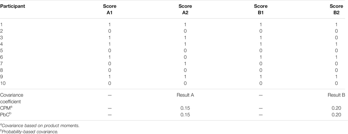
TABLE 1. Example Data Together With the Covariances Computed Using Product-moments (CPM) and Probabilities (PbC).

Table 1 lists the binary responses of ten fictitious participants who completed four items (A1, A2, B1, B2). The lower part provides the results of computing the covariances based on product-moments and probability-based covariances of A1 and A2 and also of B1 and B2. The covariance of A1 and A2 is 0.15, irrespective of the computation method. The covariance of B1 and B2 is 0.20 when computed by each one of the two computation methods.

The Skewness Problem

Skewness is a characteristic of dichotomous data if the probability of falling into one of the two possible groups of observations in dichotomization deviates from 0.5. Skewness of data is a problem since skewed data are likely to lead to incorrect results in CFA [12, 13]. Skewness means a distortion of the variances and covariances serving as input in the sense of shrinkage. Starting from a normally or binomially distributed random variable, generation of skewness implies a shift of the peak of the distribution in the direction of one of the two tails. This shift is usually associated with a decrease of the variance.

The reversal of the effect of skewness on variances and covariances can prevent the distorting influence of skewness on the outcome of confirmatory factor analysis. There are variance-stabilizing transformations that can be selected for this purpose [14–16]. Such transformations are expected to yield constancy of the variance despite deviations of the probability from 0.5. Furthermore, there is the possibility to employ a link function to overcome the difference between the distribution of data and the distribution that is expected by the statistical procedure [17–19]. CFA, which is mostly conducted according to the maximum likelihood estimation method, expects normally distributed data (or at least symmetrically distributed data). Link transformations for achieving normality focus the mean of a data distribution and are expected to transform the distribution accordingly.

Furthermore, there is also the possibility to retain the original (unchanged) variances and covariances as input to factor analysis and to adapt the statistical model to the skewness of the data. This can be achieved via the predictor-focused way of adapting the model to the probability selected for splitting data in dichotomization [20]. Adaptation of the model to theory-based expectations is also a characteristic of growth-curve modeling [21, 22]. This way of adaptation can be realized by introducing an item-specific weight w_i (i = 1, … , p) defined as function of the probability (Pr) of the response X to item i (i = 1, … , p), $X_i\left(X_i\in \left\{\mathrm{0,1}\right\}\right)$), such that

$w_i=\sqrt{\mathrm{Pr}\left(X_i=1\right)\times \left[1-\mathrm{Pr}\left(X_i=1\right)\right]}(9)$

[23]. The weight is at its maximum value for the probability of 0.5 and approaches zero for probabilities of 0 and 1.

Such weights need to be integrated into the CM model Eq. 1. Since errors are assumed to follow the normal distribution, the assignment of weights is restricted to the systematic component of the model. At first, the weights are inserted in the p×p diagonal matrix W. Afterwards, W is integrated into the CM model such that

$\Sigma =\left(W\lambda \right)\varphi \left(W\lambda \right)\prime +\theta .(10)$

The CM model specified this way expects probability-based covariances Eq. 8 as input.

The Hypotheses

In this section hypotheses suggesting constancy of the latent structure despite dichotomization are specified. We consider two types of constancy: exact constancy and relative constancy. As already pointed out, the focus is on the amount of systematic variation that is captured by the factor loadings [3] and summarized by the variance of the latent variable [8]. In CFA the variance of the latent variable can be estimated by variance parameter $\phi \ast$ if it is scaled to represent the sum of squared factor loadings (see Eqs. 2, 4, 6). Exact constancy of the scaled estimates of the variance parameter despite dichotomization means that corresponding values are achieved in investigating normally distributed data [N (0, 1)] and dichotomous data [B (1, p)]. This hypothesis is formalized by the following equation:

${\varphi }_{N\left(\mathrm{0,1}\right)}\ast ={\varphi }_{B\left(1,p\right)}\ast .(11)$

Failure to demonstrate exact constancy Eq. 11 does not necessarily mean that dichotomous data originating from interval-level data show a structure that completely differs from the structure characterizing interval-level data. Dichotomization could cause a systematic modification of structure. In such a case it should be possible to identify function g ( ) that describes the relationship between the factor loadings contributing to the variance estimates for interval-level and dichotomous data. We formalize this hypothesis suggesting relative constancy as

${\varphi }_{N\left(\mathrm{0,1}\right)}\ast ={\varphi }_{g\left(X\right)\sim N\left(\mathrm{0,1}\right),X\sim B\left(1,p\right)}\ast .(12)$

An Empirical Study Using Simulated Data

To investigate the influence of dichotomization on the latent structure of data, an empirical study was conducted. One aim of this study was to provide evidence either in favor or against the hypothesis of exact constancy of the latent structure despite dichotomization. There was also a complementary aim for the case of failure to provide confirming evidence. This aim required the recovery of the original latent structure on the basis of the information on the latent structure characterizing the dichotomous data.

Interval-level data were transformed into dichotomous data by dichotomization for the purpose of this study. To control possible error influence, two important sources of disturbance were varied. First, since dichotomization can be realized by applying various splits leading to different probabilities of the target response, several different splits were included in the design of the study. Second, since there might be different degrees of efficiency in capturing systematic variation depending on the expected amount of systematic variation, the amount of such variation was varied. Both the interval-level data and the dichotomous data were investigated by the same one-factor confirmatory factor model.

Method

Continuous and normally distributed random data [N (0,1)] were generated using PRELIS [24]. Dichotomous data showing a binomial distribution [B (1, p)] were realized by dichotomizing the continuous data using different splits so that five different probabilities of the target response (that was 1; using 0 and 1 as codes) were obtained (p = 0.2, 0.35, 0.5, 0.65, 0.8). Subsequently, the continuous and normally distributed random data [N (0,1)] were scaled down to N (0.0.25) to show a size of variance corresponding to the size of the variance of X ∼ B (1, 0.5).

The latent structure was created by means of three 20 × 20 and three 10 × 10 relational patterns. The off-diagonal entries of these patterns corresponded to the squared factor loadings. In one relational pattern the size of the factor loadings was 0.35 and in the other patterns 0.5 and 0.65. The entries of the main diagonal were ones. Since the three sizes of factor loadings could be perceived as due to latent sources with different impacts on responding, we addressed them as weak, medium and strong sources.

The data generated according to the design of the study included 400 × 3 (relational patterns) × 2 (numbers of columns) data matrices of continuous and normally distributed data and 400 × 3 (relational patterns) × 2 (numbers of columns) × 5 (probability levels) data matrices of dichotomous and binomially distributed data. A data matrix included 500 rows and either 10 or 20 columns.

The CFA model for investigating the data included one latent variable (= factor) and either 10 or 20 manifest variables. Because of the off-diagonal entries of the relational patterns showing equal sizes, the underlying structure of the data could be expected to be reproducible by factor loadings constrained to equal sizes. This expectation justified the assignment of numbers of equal size to the entries of the vector of the factor loadings in the first step. In the second step, there was scaling by transforming the factor loadings according to Eq. 4 so that the variance parameter could be expected to provide an estimate of the variance of the latent variable. Covariances based on product-moments in the case of interval-level data and probability-based covariances in the case of dichotomous data served as input to confirmatory factor analysis (see Eqs. 7, 8). There was no correction for random deviations from exact normality of generated data.

We used the maximum likelihood estimation method via LISREL [25] for investigating the data. It required continuous data, invertibility and positive definiteness; the data could be expected to be in line with these requirements. Furthermore, there is the difference between the binomial distribution of the data and the normal distribution of the latent variables of the models that is likely to lead to model misfit. It was overcome by the transformation of factor loadings that means by adaptation of model to data. This transformation was realized using the item-specific weights w_i (see Eqs. 9, 10). Since the major characteristics of the model were in line with the major properties of the generated data, good model fit could be expected. Therefore, the results section does not include a report of the fit results. Instead, the focus of the investigation is on the size of the variance parameter regarding the exact constancy hypothesis and on the size of factor loadings regarding the relative constancy hypothesis. Variance estimates and factor loadings are reported.

Results

Results for continuous and normally distributed data. The variance estimates and standard deviations of latent variables observed in investigating continuous data showing the normal distribution are reported in Table 2.

TABLE 2

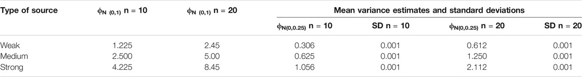
TABLE 2. Mean Variance Estimates and Standard Deviations of Latent Variable Observed in Investigating Interval-level Data with Variances of 0.25 for Datasets with 10 and 20 Columns (400 Datasets).

The first column of this table lists the sources and the second and third columns the sizes of factor loadings for standard normal data [N (0.1)]. The fourth and fifth columns provide the mean variance estimates and corresponding standard deviations observed in investigating data matrices of datasets with 10 columns showing a variance of 0.25 [N (0.0.25)]. The sixth and seventh columns comprise the corresponding means and standard deviations observed in investigating matrices of datasets with 20 columns.

The mean variance estimates varied between 0.306 and 2.112. There was a linear increase from weak to strong. Furthermore, the means observed in investigating matrices of datasets with 10 and 20 columns differed systematically, as is suggested by Eq. 2 (2 × ϕ∗_n=10 = ϕ∗_n=20). Moreover, the comparison of the variance estimates obtained for data with distributions N (0,1) and N (0.0.25) revealed a decrease from 100 to 25 percent. All standard deviations were very small. Apparently, a reduction of the variance of normally distributed data for 100 to 25 percent was associated with a corresponding reduction of the variance of the latent variable.

Results for binary and binomially distributed data. Table 3 provides the results observed in investigating dichotomous data.

TABLE 3

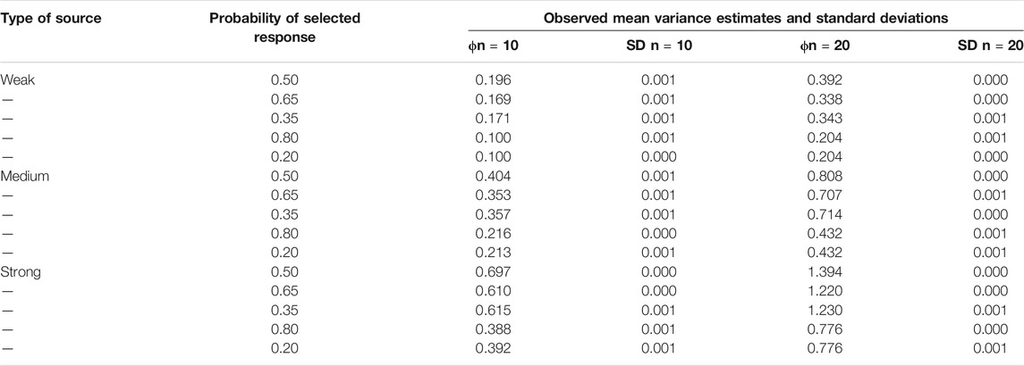
TABLE 3. Mean Variance Estimates and Standard Deviations of Latent Variables Observed in Investigating Dichotomous Data for Datasets with 10 and 20 Columns (400 Datasets).

The first column of this table gives the type of source and the second column the probability level. The mean variance estimates are provided in the third and fifth columns. The results for datasets with 20 columns virtually always showed double the size of the results for datasets with 10 columns. Since no difference between the double of an estimate reported in column 3 and the corresponding estimate reported in column 5 was larger than 0.008, in the following the discussion of the results does not specify the number of columns of the datasets that were investigated.

The variance estimates varied between 0.100 and 1.394. For each type of source (weak, medium, strong) there was a decrease in the size of the variance from the first to fifth rows (i.e., from p = 0.5 to p = 0.2/0.8). The decrease occurred stepwise from the variance estimate for the probability level of 0.5 to the variance estimates of the levels of 0.35 and 0.65 in the first step down and to the variance estimates of the levels of 0.2 and 0.8 in the second step down. Furthermore, the variance estimates for the probability levels 0.35 and 0.65 and also for the probability levels 0.2 and 0.8 differed by a very small amount only. Regarding the influence of the type of source, there was an increase in the size of the variance of the latent variable from the weak to strong sources. All standard deviations were very small.

Comparison of the results for normally and binomially distributed data. Table 4 relates the variance estimates obtained for continuous and normally distributed data [N (0.0.25)] (see Table 2) to the variance estimates obtained for dichotomous and binomially [B (1.0.5)] distributed data (see Table 3). This comparison was restricted to variance estimates obtained from data with variances of 0.25 to make the effect of dichotomization especially obvious.

TABLE 4

TABLE 4. Ratios of Variance Estimates for Interval-level Data and Dichotomous Data Showing the Variance of 0.25 for Datasets with 10 and 20 Columns (400 Datasets).

The first and second columns of this Table provide the variance estimates for interval-level data showing the normal distribution [N (0.0.25)]. The means of the variance estimates for dichotomous and binomially distributed data originating from dichotomization with the probability level of 0.5 are included in the fourth and sixth columns. Furthermore, ratios of the values included in the first and fourth respectively the second and sixth columns are reported in the fifth and seventh columns.

The ratios varied between 1.51 and 1.56. The differences between the ratios were small, suggesting a small effect of the strength of source. The ratios suggested that there was an increase in the retained systematic variation.

In sum, the results did not confirm the hypothesized constancy of the latent structure of data despite dichotomization in the sense of exact constancy (see Eq. 11). However, the deviation from exact constancy appeared to occur in a systematic way that suggested the possibility of relative constancy (see Eq. 12). The deviation appeared to be associated with the probability of splitting the data in dichotomization, and the strength of the source also appeared to influence the results.

The Shrinkage Correction

This section describes easy ways of recovering the latent structure of interval-level data on the basis of dichotomous data and provides an evaluation of these ways. The investigation is conducted at the level of factor loadings since the effect of dichotomization characterized the columns of the dataset that were split in dichotomization in the first place. Furthermore, the transformations leading to the recovery of the original factor loadings occurred at this level.

In order to eliminate probability level-related deviations (the differences between factor loadings based on the same source but differing according to the probability of the target response), a ratio of products of variances for p_o = 0.5 and other ps is computed and used as multiplier of the factor loadings:

${\lambda }_{\text{D}.\text{PC}}=\frac{p_o\left(1-p_o\right)\times \left[1-p_o\left(1-p_o\right)\right]}{p\left(1-p\right)\times \left[1-p\left(1-p\right)\right]}\times {\lambda }_D(13)$

where λ_D represents the observed factor loading for dichotomous data and λ_D.PC the factor loading corrected for the probability-based deviation from p = 0.5.

For compensating the shrinkage from interval-level data to dichotomous data, two types of shrinkage correction were worked out. First, we considered the correction by shrinkage coefficient c_S. For the purpose of relating factor loadings computed from dichotomous data [B (1,p)] to factor loadings computed from standard normal data [N (0.1)], we also computed the ratios that were 2.50 for the weak type of source, 2.485 for the medium type of source and 2.46 for the strong type of source. These ratios surmounted the ratios reported in Table 4 because of the switch from [N (0.0.25)] to [N (0.1)]. The simplicity principle led us to select 2.5 as shrinkage coefficient (c_S = 2.5) so that

${\lambda }_{\text{D}.\text{PC}.\text{SC}}=c_{\text{S}}\times {\lambda }_{\text{D}.\text{PC}}(14)$

where λ_D.PC represented the factor loading corrected for the probability-based deviation (see Eq. 13) and λ_D.PC.SC the factor loading additionally corrected by the effect of the type of source. This correction coefficient could be perceived as the square root of the ratio of squares of factor loadings for interval-level and dichotomous data [λ_N(0,1) and λ_B(1,0.5)] of the weak source:

$c_{\text{S}}=\sqrt{\frac{{\lambda }_{N\left(\mathrm{0,1}\right)}^2}{{\lambda }_{B\left(\mathrm{1,0.5}\right)}^2}}(15)$

Second, a simple function was also considered for accomplishing the shrinkage correction. It included weights of 2.54 and -0.32 assigned to the linear and quadratic terms of a quadratic polynomial for correcting the shrinkage:

${\lambda }_{\text{D}.\text{PC}.\text{SF}}=2.54\times {\lambda }_{\text{D}.\text{PC}}-0.32\times {\lambda }_{\text{D}.\text{PC}}^2(16)$

where λ_D.PC represented the factor loading corrected for the probability-based deviation and λ_D.PC.SF the factor loading with the additional shrinkage correction. It needs to be added that using the results of the simulation study for working out the correction methods implicitly restricted their applicability to the investigated ranges of factor loadings and probability levels.

We evaluated the two ways of recovering the latent structure by attempts to reproduce the factor loadings for interval-level data following the standard normal distribution. In these attempts we started from the factor loadings reported in Table 3 for dichotomous data. The calculated shrinkage-corrected factor loadings rounded to the two positions following the comma are reported in Table 5.

TABLE 5

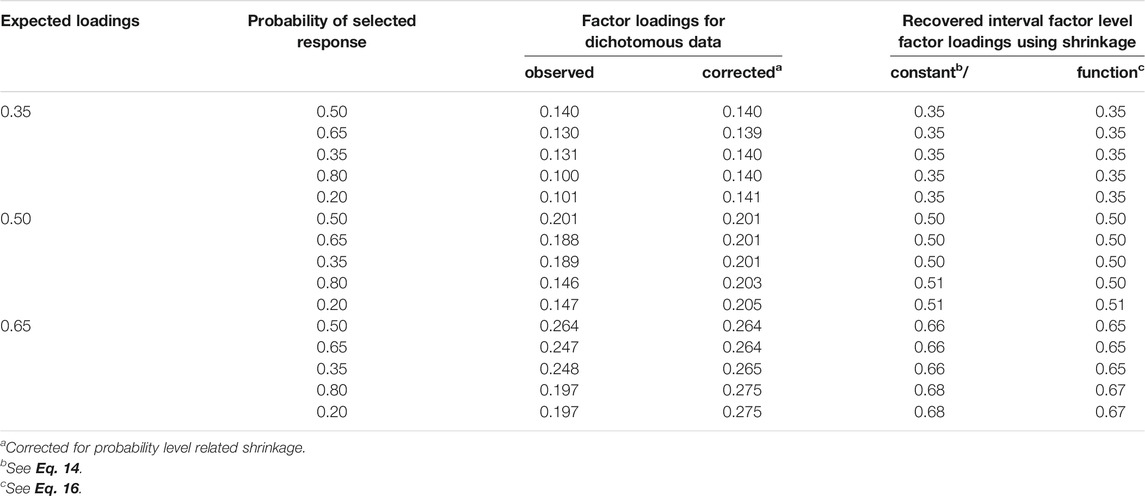
TABLE 5. Observed and Probability-corrected Factor Loadings for Dichotomous Data as Well as Recovered Factor Loadings for Interval-level Data (400 Datasets).

The first column provides the expected factor loadings, the second column the probabilities of the target response and the third column the factor loadings observed in investigating dichotomous data (the means of estimates reported for 10 and 20 manifest variables in Table 3). The results of transformations according to Eq. 13 are included in the fourth column, according to Eq. 14 in the fifth column and according to Eq. 16 in the sixth column, respectively.

The correction for probability-related deviations Eq. 13 led to factor loadings that showed similar sizes for the same source but were not exactly equivalent (eliminating the third digit would only reveal equivalence for the weak and medium sources). Using the shrinkage coefficient described by Eq. 14 provided factor loadings according to expectation for the weak source. For the medium and strong sources there were deviations up to 0.01 and 0.03, respectively. Using the shrinkage correction described by Eq. 16 reduced the number of deviations from expectations. There were only three instead of seven deviations and the largest deviation was 0.02.

It remains to report the effect of shrinkage correction on the factor loadings reported in the introduction. The shrinkage correction transformed the values of 0.20, 0.19, 0.22 and 0.18 into values of 0.58, 0.60, 0.55 and 0.61.

Discussion

The information on the latent structure of data collected by a measurement scale is used for evaluating its quality. The procurement of such information is considered as an essential part of test construction [26, 27]. Therefore, it is of great importance that the information on the latent structure is free of any bias and method effect [11]. This argument also extends to shrinkage due to dichotomization that either occurs during measurement or as a post-hoc transformation. Therefore, it is worthwhile to investigate the effect of dichotomization and to engage into the search for a way of reversing it.

An investigation of the latent structure yields information on the dimensionality and systematic variation characterizing data. The reported study concentrates on the investigation of the effect of dichotomization on the amount of systematic variation. This research strategy deviates from typical data analysis by a CFA model that seeks to provide confirmation of the appropriateness of the pre-specified model of measurement [28]. This deviation is justified by the high degree of correspondence of the models employed for data generation and for data analysis. In addition, there were occasional checks regarding model fit during the simulation study that would reveal deviations from the expected dimensionality.

The comparison of factor loadings for interval-level and dichotomous data suggested shrinkage of the systematic variation due to dichotomization. This result is no surprise since in dichotomization exact information on the (fictitious) participants is replaced by information on the category to which the (fictitious) participants are assigned. The information is inexact in that it is an inexact characterization of the (fictitious) participants. But, this does not mean that the information is wrong or represents random influences only.

Inexact information on individual participants does not preclude the achievement of exact information on the sample. Counting the target responses in the sample and turning them into probabilities provides information that is considered interval-level information. It is used for computing probability-based covariances [29]. The probabilities achieved this way still reflect the influence of the probability levels used in splitting the original interval-level data so that it is necessary to take care of the associated skewness, as is outlined in previous sections. Furthermore, the accuracy of the information depends on sample size. Increasing the sample size increases the degree of accuracy, as is suggested by the central limit theorem [30].

The simulation study includes attempts to recover the values for factor loadings of interval-level data according to Eqs. 13–16 using the readily available information. The results are generally good but also show small deviations from what is expected. The recovery was very accurate if the data were constructed to reflect a weak latent source. If the latent source was simulated to show medium strength, it was also very accurate with one exception. Small overestimation characterizes the recovery in the case of the strong simulated source. So, it turns out that the information on the systematic variation can largely be recovered despite the loss of information on the (fictitious) participants. This suggests that dichotomization is a systematic transformation of data that retains general characteristics.

Further studies may show whether the deviations are simply inaccuracies or an indication of another influence that has not been considered so far. Moreover, although broad ranges of probabilities and sizes of factor loadings of relevance have been considered, generalization to the full ranges should be based on the results of a more complete investigation. Further investigations may confirm and extend the results of the reported study.

Conclusion

Dichotomization of data causes shrinkage of the latent variance of data that means an impairment of the latent structure of data. The shrinkage occurs in a systematic way so that recovery of the original latent variance is possible.

Data Availability Statement

The datasets presented in this article are not readily available because only the starting numbers were saved, not the generated data. The starting numbers of the generated data sets can be made available to fully reproduce the data. Requests to access the datasets should be directed to KS, k.schweizer@psych.uni-frankfurt.de.

Author Contributions

KS conceptualized the study and contributed to the writing. AG and DK contributed substantially to the writing. All authors contributed to the article and approved the submitted version.

Conflict of Interest

The authors declare that the research was conducted in the absence of any commercial or financial relationships that could be construed as a potential conflict of interest.

Publisher’s Note

All claims expressed in this article are solely those of the authors and do not necessarily represent those of their affiliated organizations, or those of the publisher, the editors and the reviewers. Any product that may be evaluated in this article, orclaim that may be made by its manufacturer, is not guaranteed or endorsed by the publisher.

References

1. Suppes, P, and Zinnes, JL. Basic Measurement Theory. In: R Luce RD, RR Bush, and EH Galanter, editors. Handbook of Mathematical Psychology. Hoboken, NJ: Wiley (1963). p. 1–76.

Google Scholar

2. Vogt, WP, and Johnson, RB. The SAGE Dictionary of Statistics & Methodology: A Nontechnical Guide for the Social Sciences. 5th ed.. Thousand Oaks, CA: Sage (2015). p. 522.

Google Scholar

3. Widaman, KF. On Common Factor and Principal Component Representations of Data: Implications for Theory and for Confirmatory Replications. Struct Equation Model A Multidisciplinary J (2018) 25:829–47. doi:10.1080/10705511.2018.1478730

CrossRef Full Text | Google Scholar

4. Brown, TA. Confirmatory Factor Analysis for Applied Research. 2n ed.. New York: The Guilford Press (2015). p. 437.

Google Scholar

5. Jöreskog, KG. A General Method for Analysis of Covariance Structures. Biometrika (1970) 57:239–57. doi:10.2307/2334833

CrossRef Full Text | Google Scholar

6. Little, TD, Slegers, DW, and Card, NA. A Non-arbitrary Method of Identifying and Scaling Latent Variables in SEM and MACS Models. Struct Equation Model A Multidisciplinary J (2006) 13:59–72. doi:10.1207/s15328007sem1301_3

CrossRef Full Text | Google Scholar

7. Schweizer, K, Troche, SJ, and DiStefano, C. Scaling the Variance of a Latent Variable while Assuring Constancy of the Model. Front Psychol (2019) 10:887. doi:10.3389/fpsyg.2019.00887

PubMed Abstract | CrossRef Full Text | Google Scholar

8. Schweizer, K, and Troche, S. The EV Scaling Method for Variances of Latent Variables. Methodology (2019) 15:175–84. doi:10.1027/1614-2241/a000179

CrossRef Full Text | Google Scholar

9. Finch, WH, and French, BF. Confirmatory Factor Analysis. In: WH Finch, and BF French, editors. Latent Variable Modeling with R. New York: Routledge (2015). p. 37–58.

Google Scholar

10. Schweizer, K, Gold, A, and Krampen, D. A Semi-hierarchical Confirmatory Factor Model for Speeded Data. Struct Equation Model A Multidisciplinary J (2020) 27:773–80. doi:10.1080/10705511.2019.1707083

CrossRef Full Text | Google Scholar

11. Maul, A. Method Effects and the Meaning of Measurement. Front Psychol (2013) 4:169. doi:10.3389/fpsyg.2013.00169

PubMed Abstract | CrossRef Full Text | Google Scholar

12. Fan, W, and Hancock, GR. Robust Means Modeling. J Educ Behav Stat (2012) 37:137–56. doi:10.3102/1076998610396897

CrossRef Full Text | Google Scholar

13. West, SG, Finch, JF, and Curran, PJ. Structural Equation Models with Non-normal Variables: Problems and Remedies. In: R Hoyle, editor. Structural Equation Modeling: Concepts, Issues, and Applications. Thousand Oaks, CA: SAGE (1995). p. 56–75.

Google Scholar

14. Yu, G. Variance Stabilizing Transformations of Poisson, Binomial and Negative Binomial Distributions. Stat Probab Lett (2009) 79:1621–9. doi:10.1016/j.spl.2009.04.010

CrossRef Full Text | Google Scholar

15. Morgenthaler, S, and Staudte, RG. Advantages of Variance Stabilization. Scan J Stat (2012) 39:714–28. doi:10.1111/j.1467-9469.2011.00768.x

CrossRef Full Text | Google Scholar

16. Yamamura, K. Transformation Using ( X + 0.5) to Stabilize the Variance of Populations. Popul Ecol (1999) 41:229–34. doi:10.1007/s101440050026

CrossRef Full Text | Google Scholar

17. McCullagh, P, and Nelder, JA. Generalized Linear Models. London: Chapman & Hall (1985). p. 250.

Google Scholar

18. Nelder, JA, and Wedderburn, RWM. Generalized Linear Models. J R Stat Soc Ser A (General) (1972) 135:370–84. doi:10.2307/2344614

CrossRef Full Text | Google Scholar

19. Skrondal, A, and Rabe-Hesketh, S. Generalized Latent Variable Modelling: Multilevel, Longitudinal and Structural Equation Models. London: Chapman and Hall/CRC (2004). p. 528.

Google Scholar

20. Schweizer, K, Ren, X, and Wang, T. A Comparison of Confirmatory Factor Analysis of Binary Data on the Basis of Tetrachoric Correlations and of Probability-Based Covariances: A Simulation Study. In: RE Millsap, DM Bolt, LA van der Ark, and WC Wang, editors. Quantitative Psychology Research. Heidelberg, Germany: Springer (2015). p. 273–92. doi:10.1007/978-3-319-07503-7_17

CrossRef Full Text | Google Scholar

21. Bollen, KA, and Curran, PJ. Latent Curve Models. Hoboken: Wiley (2006). p. 285.

Google Scholar

22. McArdle, JJ. Latent Variable Modeling of Differences and Changes with Longitudinal Data. Annu Rev Psychol (2009) 60:577–605. doi:10.1146/annurev.psych.60.110707.163612

PubMed Abstract | CrossRef Full Text | Google Scholar

23. Zeller, F, Reiss, S, and Schweizer, K. Is the Item-Position Effect in Achievement Measures Induced by Increasing Item Difficulty. Struct Equation Model A Multidisciplinary J (2017) 24:745–54. doi:10.1080/10705511.2017.1306706

CrossRef Full Text | Google Scholar

24. Jöreskog, KG, and Sörbom, D. Interactive LISREL: User’s Guide. Lincolnwood, IL: Scientific Software International Inc (2001). p. 378.

Google Scholar

25. Jöreskog, KG, and Sörbom, D. LISREL 8.80. Lincolnwood, IL: Scientific Software International Inc (2006).

Google Scholar

26. Lord, FM, and Novick, MR. Statistical Theories of Mental Test Scores. Reading, MA: Addison-Wesley (1968). p. 568.

Google Scholar

27. McDonald, RP. Test Theory: A Unified Treatment. Lawrence Erlbaum Associates (1999). p. 400.

Google Scholar

28. Graham, JM. Congeneric and (Essentially) Tau-Equivalent Estimates of Score Reliability. Educ Psychol Meas (2006) 66:930–44. doi:10.1177/0013164406288165

CrossRef Full Text | Google Scholar

29. Schweizer, K. A Threshold-free Approach to the Study of the Structure of Binary Data. Ijsp (2013) 2:67–75. doi:10.5539/ijsp.v2n2p67

CrossRef Full Text | Google Scholar

30. Fischer, H. A History of the Central Limit Theorem. Heidelberg: Springer (2011).

Google Scholar