Stability Analysis of a Modified Leslie–Gower Predation Model With Weak Allee Effect in the Prey

1. Introduction

Predator-prey models are studied in both applied mathematics [1–3] and ecology [4–7]. The goal of these studies is to describe and analyse the predation interaction between the predator and the prey and predict how they respond to future interventions [8, 9]. These studies often use mathematical models to describe the species' interactions and the time-series behaviors [10, 11]. The models aim to be representative of real natural phenomena capturing the essentials of the dynamics. However, new technologies used to study biological and physical phenomenon reveal that species' interactions are more complex than previously used in the models [7, 12–14]. The importance of these more complex interactions are becoming increasingly apparent as research findings have shown that ecosystem dynamics depend on the particular nature of the interaction processes, such as the functional response and predation rate [6, 7, 15, 16].

A standard approach for using models to understand ecological systems is to design a framework based on simple principles and compare species' abundance that result from the predicting analysis of those models. However, this approach becomes more difficult when additional nuances to standard models are added, making them more complex and difficult to analyse. For instance, Graham and Lambin [17] showed that field-vole (Microtus agrestis) survival can be affected by reducing least weasel (Mustela nivalis) predation. They also demonstrated that weasels were suppressed in summer and autumn, while the vole (Microtus agrestis) population always declined to low density. However, the authors argued that the underlying model was too difficult to study due to a large number of parameters.

The model used by Graham and Lambin in [17] is a Leslie–Gower predator-prey model [18] and is given by

$\begin{array}{ll}\begin{array}{l}\frac{dN}{dt}=rN\left(1-\frac{N}{K}\right)-\frac{qNP}{N+a},\\ \frac{dP}{dt}=sP\left(1-\frac{P}{hN}\right).\end{array}& (1)\end{array}$

Here, N(t) > 0 and P(t) > 0 are used to represent the size of the prey and predator population at time t, respectively. The prey population grows logistically with carrying capacity K and intrinsic growth rate r. The growth of the predator is also logistic, with intrinsic growth rate s, but the carrying capacity is prey dependent and h is a measure of the quality of the prey as food for the predator. The functional response is Holling type II where q is the maximum predation rate per capita and a is half of the saturated response level [7].

In population dynamics, many ecological mechanisms are connected with individual cooperation such as strategies to hunt, collaboration in unfavorable abiotic conditions and reproduction [19]. An example of such an ecological mechanism is the cooperative interaction observed in Kakapo (Strigops habroptilus). This interaction can be influenced by reducing the fecundity levels and the population size [20]. Another factor that affects the population dynamics is the species density. For instance, when the predator population size is low they have more resources and benefits. However, there are species that may suffer from a lack of conspecifics, which may be less likely to reproduce or survive in a small-sized population [21]. In these instances, the size of the population is important, as for a smaller size of biomass adaptability may be diminished [20]. When Allee and collaborators [22] analyzed the data of the false weevil (Tribolium confusum) they observed that the highest growth rates of their populations per capita were at intermediate densities [20]. The fact that they were lower in high densities was not surprising, as intraspecific competition is high. In contrast, when fewer males were present, females produced fewer eggs, which is not an obvious correlation for an insect. In this case, optimal egg production was thus achieved at intermediate densities. This effect is now referred to as the Allee effect [22, 23]. It is modeled by incorporating the factor (N − m) into the logistic equation, with the idea that when the prey population N decreases below the Allee threshold m > 0 the prey rate of growth becomes negative, indicating signs of extinction. Therefore, the prey logistic growth r(1 − N/K) is replaced by r(1 − N/K)(N − m). For 0 < m < K, the per-capita growth rate of the prey population with the Allee effect included is negative, but increasing, for N ∈ [0, m), and this is referred to as the strong Allee effect. When m ≤ 0, the per-capita growth rate is positive but increases at low prey population densities and this is referred to as the weak Allee effect [20, 23]. With the Allee effect included, the Leslie–Gower predator-prey model (1) of [17] becomes

$\begin{array}{ll}\begin{array}{l}\frac{dN}{dt}=rN\left(1-\frac{N}{K}\right)(N-m)-\frac{qNP}{N+a}=N·W(N,P),\\ \frac{dP}{dt}=sP\left(1-\frac{P}{hN}\right)=P·R(N,P).\end{array}& (2)\end{array}$

The aim of this manuscript is to study the Leslie–Gower predator-prey model with weak Allee effect on prey, that is (2) with m < 0. By considering a weak Allee effect in the prey population we complement the results of Ostfeld and Canhan [24]. The authors studied the stabilization of a file-vole population which depends on the variation in reproductive rate and recruitment of the population, i.e., an Allee effect. The weak Allee effect can be also observed in the File-vole species as the survival rate for adults were delayed [24]. However, these phenomena were not considered by the authors as they used model (1). This manuscript also extends some of the results obtained by Arancibia–Ibarra and González–Olivares [25] and González–Olivares et al. [26] for a modified Leslie–Gower model with m = 0, that is, with a specific type of weak Allee effect, see second row of Table 1. Leslie–Gower models with strong Allee effect and different type of functional responses have been extensively studied in [27–29], see first row of Table 1. In these articles the authors showed that the system, for certain system parameters, supports the extinction of both species and it also supports the stabilization of both populations over the time, i.e., coexistence. Moreover, system (2) with m < 0 complements the results of the Leslie–Gower model studied by Courchamp et al. [20]. The authors in [20] argue that the Allee effect in prey generally destabilizes the dynamics between the prey and the predator. Moreover, the Allee effect can prevent the oscillation of both populations. However, in this manuscript, we find that the Leslie–Gower model with weak Allee effect supports the coexistence and oscillation of both populations.

TABLE 1

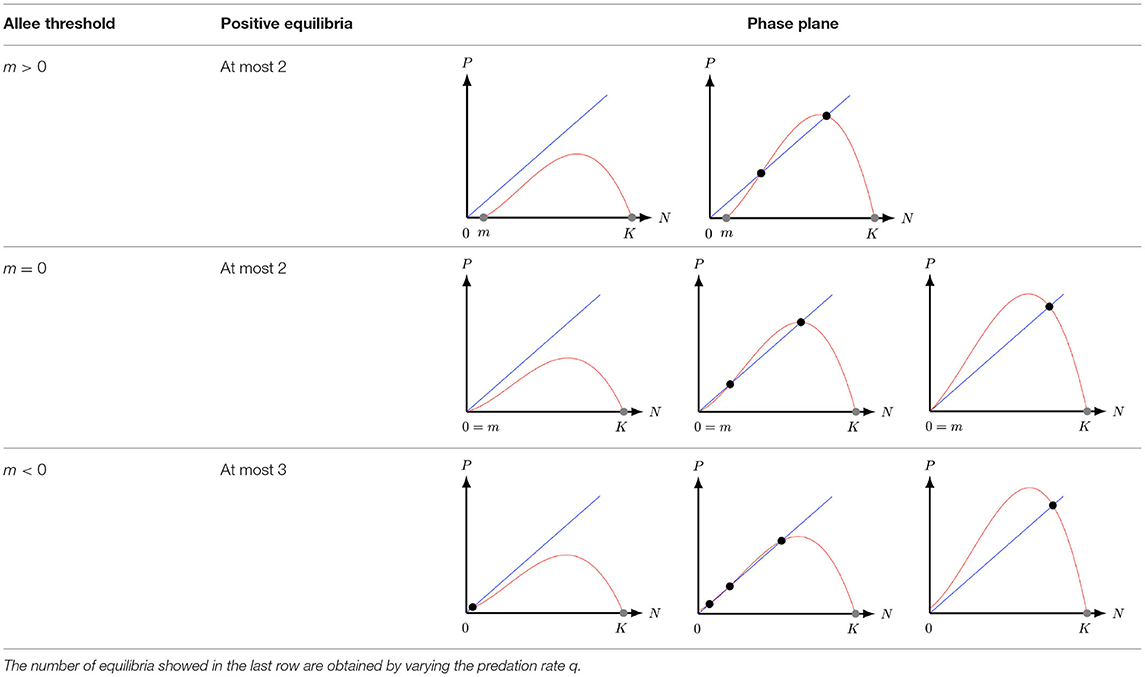
Table 1. Number of equilibria of system (2) with strong (m > 0), degenerate weak (m = 0), and weak (m < 0) Allee effect.

In section 2, we non-dimensionalise the Leslie–Gower model with weak Allee effect and discuss the number of equilibria the model has in the first quadrant. The main mathematical difference between system (1), (2) with m < 0, and (2) with m ≥ 0, is the fact that (2) with m < 0 has at most three positive equilibria¹ in the first quadrant instead of one for system (1) and two for system (2) with m ≥ 0 [25, 26, 29]. These additional equilibrium gives rise to different type of bifurcations, such as saddle-node bifurcations, Bogdanov–Takens bifurcations, and homoclinic bifurcations. The main properties of the equilibria are studied in section 3. In particular, we study the stability of the equilibria and present the conditions for which the model undergoes different type of bifurcations. Finally, in section 4, we summarize the results and discuss the ecological implications of the model.

2. The Model

The Leslie–Gower model with weak Allee effect is given by (2) with m < 0, and we only consider the model in the domain Ω = {(N, P) ∈ ℝ², N > 0, P ≥ 0} and $(r,K,q,a,s,h)\in {ℝ}_{+}^6$. The axes in system (2) are invariant since (2) is of Kolmogorov type [30] (i.e., dN/dt = N · W(N, P) and dP/dt = P · R(N, P)). The equilibria of system (2) are (K, 0) and (x*, y*), which are the intersections of the nullclines

$P=hN\text{and}P=\frac{r}{q}\left(1-\frac{N}{K}\right)(N+a)(N-m).$

We follow the non-dimensionalisation approach of [29] to simplify the analysis and remove the N = 0 singularity for the model. We introduce $\bar{\Omega }=\{(u,v)\in {ℝ}^2,u\ge 0,v\ge 0\}$ and the dimensionless variables (u, v, τ) given by

$\begin{array}{ll}\begin{array}{l}\phi :\bar{\Omega }\times ℝ\to \Omega \times ℝ\text{where}\phi (u,v,\tau )\\ =\left(\frac{N}{K},\frac{P}{hK},\frac{rKt}{u\left(u+\frac{a}{K}\right)}\right).\end{array}& (3)\end{array}$

Observe that φ (3) is a diffeomorphism which preserve the orientation of time [31, 32]. Next, set A: = a/K ∈ (0, 1), S: = s/(rK), Q: = hq/(rK) and M: = m/K, then (2) transforms into the non-dimensionalised system

$\begin{array}{ll}\begin{array}{l}\frac{du}{d\tau }=u^2((u+A)(1-u)(u-M)-Qv),\\ \frac{dv}{d\tau }=S(u+A)(u-v)v.\end{array}& (4)\end{array}$

The u-nullclines of system (4) are given by u = 0 and v = (u + A)(1 − u)(u − M)/Q, while the v-nullclines of interest are given by v = 0 and v = u. Hence, the equilibria of system (4) are (0, 0)², (1, 0), and the positive equilibria (u*, v*) with v* = u* and where u* is determined by the solution(s) of (u + A)(1 − u)(u − M)/Q = u, or, equivalently,

$\begin{array}{ll}g(u):=u^3-T(A,M)u^2-L(A,M,Q)u+AM=0,& (5)\end{array}$

with T(A, M) = 1 − A + M and L(A, M, Q) = A(M + 1)−Q−M. Since g(0) = AM < 0 and g(1) = Q > 0, there is always at least one positive equilibrium (u*, u*) with 0 < u* < 1. To obtain information about potential other positive equilibria, we divide (5) by (u − u*) and obtain the quadratic equation

$\begin{array}{ll}{u}^2+u(u^{*}-T(A,M))+u^{*}(u^{*}-T(A,M))-L(A,M,Q)=0.& (6)\end{array}$

Note that as system (4) is topologically equivalent to system (2), the solution u* of (5) is related to a population equilibrium of system (2). Therefore, a positive equilibrium point P = (u*, u*) in system (4) correspond to a coexisting equilibrium point in system (2).

Lemma 2.1. The positive roots of g(u) (5) lie in (0, 1), and

  (I) if T(A, M) ≤ 0 or L(A, M, Q) ≥ 0, then g(u) (5) has one positive root and system (4) thus has one positive equilibrium, see Figures 1A,E.

(II) if T(A, M) > 0, L(A, M, Q) < 0 and

(i) Δ < 0, where Δ is the discriminant of (6) (with respect of the dependent variable u) given by

$\begin{array}{l}\Delta :={\left(u^{*}-T(A,M)\right)}^2-4(u^{*}\left(u^{*}-T(A,M)\right)\\ -L(A,M,Q)),& (7)\end{array}$

then g(u) (5) has one positive root and system (4) thus has one positive equilibrium, see Figures 1A,E;

(ii) Δ ≥ 0 (7), then g(u) (5) has three roots (counting multiplicity) and system (4) thus has three positive equilibria, see Figures 1B–D.

Proof: The cubic equation g(u) (5) always has at least one root in (0, 1), since g(0) = AM < 0 and g(1) = Q > 0, and the first case of the lemma, case 1, thus immediately follows from Descartes' rule of signs ([33], e.g.).

FIGURE 1

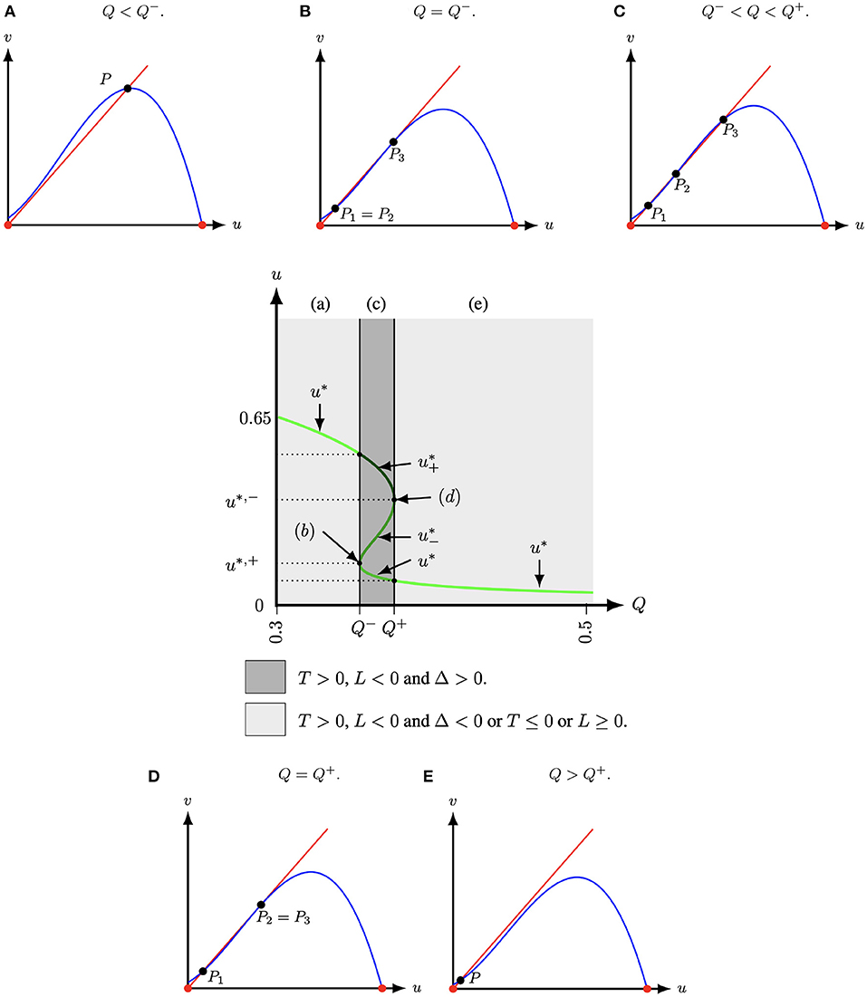
Figure 1. The schematic diagram of the number of positive roots of Equation (5) in the (u, Q)-space for (A, M) = (1/10, −1/10) fixed and with T = 1 − A + M, L = A(M + 1) − Q − M, Δ = (u* − T(A, M))² − 4(u*(u* − T(A, M)) − L(A, M, Q)) and u* is determined by the solution(s) of (5). At $Q=Q^{\pm }:=(73\pm \sqrt{5})/200$, that is, at Q⁻ ≈ 0.35381966 and Q⁺ ≈ 0.376180, two positive equilibria collapse. For Q < Q⁻ or Q > Q⁺, Equation (5) has only one positive root (light grey regions). Hence, system (4) has only one positive equilibrium P = (u*, u*). For Q⁻ < Q < Q⁺, Equation (5) has three positive roots (dark grey region) and system (4) thus has three positive equilibria. (A) Q < Q⁻. (B) Q = Q⁻. (C) Q⁻ < Q < Q⁺. (D) Q = Q⁺. (E) Q > Q⁺.

Case (II)(i) also follows directly from Descartes' rule of signs, which for T(A, M) > 0 and L(A, M, Q) < 0 states that g(u) (5) has one or three positive roots (counting multiplicity), and the observation that the quadratic equation 5 has two complex roots as its discriminant is negative.

In the last case, case (II)(ii), g(u) (5) has three real roots: u* and

$\begin{array}{ll}\begin{array}{l}{u}_{-}^{*}=\frac{1}{2}\left(T(A,M)-u^{*}-\sqrt{\Delta }\right),\\ u_{+}^{*}=\frac{1}{2}\left(T(A,M)-u^{*}+\sqrt{\Delta }\right).\end{array}& (8)\end{array}$

The latter two being the roots of (6). What remains to show is that $u_{\pm }^{*}\in (0,1)$. To show this, we look at the derivative of g(u)

$g^{\prime }(u)=3u^2-2T(A,M)u-L(A,M,Q).$

The assumptions T(A, M) > 0 and L(A, M, Q) < 0 imply that g′(u) ≥ 0 for u ≤ 0. Furthermore, T(A, M) ∈ (0, 1) and, for u ≥ T, we thus also get

$\begin{array}{l}{g}^{\prime }(u)=3u^2-2T(A,M)u-L(A,M,Q)>2u(u-T(A,M))\\ +u^2>2u(u-T(A,M))\ge 0.\end{array}$

In other words, under the assumptions T(A, M) > 0 and L(A, M, Q) < 0, the cubic function g(u) is strictly increasing outside the interval (0, T(A, M)) (with T(A, M) < 1). Since g(0) = AM < 0 and g(1) = Q > 0, it thus follows that $u_{\pm }^{*}\in (0,1)$.□

We observe that none of these equilibria explicitly depend on the system parameter S. Moreover, only L(A, M, Q) in g(u) (5) depends directly on Q. Therefore, S and Q are natural candidates to act as bifurcation parameters. For instance, when two of the three roots of g(u) coincide, say $u_{-}^{*}$ and $u_{+}^{*}$, we change from having three roots to one root (upon changing Q). So, at this point we have

$\begin{array}{l}{u}_{-}^{*}=u_{+}^{*}\Rightarrow u^{*}=u^{*,\pm }\\ :=\frac{1}{3}\left(T(A,M)\pm 2\sqrt{T{(A,M)}^2+3L(A,M,Q)}\right).\end{array}$

Implementing this into g(u^*,±) = 0 results in an analytic implicit expression Q = Q^±(A, M) at which the number of roots changes. For example, for (A, M) = (1/10, −1/10) as in Figure 1 we get $Q^{\pm }(1/10,-1/10)=(73\pm \sqrt{5})/200$.³

In case (II)(ii) of Lemma 2.1 we find that g(u) has three roots in (0, 1): u* and $u_{\pm }^{*}$ (8), with $u_{-}^{*}\le u_{+}^{*}$. The latter two roots depend on the first root u*, but, a priori, we do not know anything about parity of $u^{*}-u_{\pm }^{*}$. However, the roots of g(u) do not depend on which of the three roots we pick a priori as u* in the lemma. Hence, we can, without loss of generality, assume in the remainder of this manuscript that $0<u^{*}\le u_{-}^{*}\le u_{+}^{*}<1$. However, see the proof of Corollary 3.3 where we utilize this independence of our initial pick.

3. Main Results

In this section, we discuss the main results related to system (4). That is, we discuss the nature of the equilibria (section 3.1) and their bifurcations (section 3.2). First we observe that from [29, Theorem 2] it instantly follows that all solutions of (4) which are initiated in the first quadrant are bounded and end up in

$\begin{array}{ll}\Phi =\{(u,v),0<u\le 1,0\le v\le 1\}.& (9)\end{array}$

3.1. The Nature of the Equilibria

To determine the stability of the equilibria on the axes of interest (0, 0) and (1, 0) we compute the Jacobian matrix of system (4)

$\begin{array}{ll}J(u,v)=\left(\begin{array}{cc}-u{J}_{11}& -Q{u}^2\\ Sv(A+2u-v)& S(u-2v)(A+u)\end{array}\right),& (10)\end{array}$

with $J_{11}=4A{u}^2-4M{u}^2+2AM-3Au+3Mu+2Qv-4u^2+5u^3-3AMu$. The determinant and the trace of the Jacobian matrix (10) are:

$\begin{array}{ll}\begin{array}{l}det(J(u,v))=-J_{11}Su(u-2v)(A+u)+QS{u}^{2}v(A+2u-v),\\ \text{ tr}(J(u,v))=-u{J}_{11}+S(u-2v)(A+u)\end{array}& (11)\end{array}$

Lemma 3.1. The equilibrium (0, 0) is a non-hyperbolic saddle point and (1, 0) is a saddle point.

Proof: Since det(J(1, 0)) = −S(1 − M)(A + 1)² < 0 it immediately follows that (1, 0) is a saddle point. To prove the results for the origin we follow the methodology used to desingularise the origin showed in ([29], Lemma 2). First, we observe that setting u = 0 in system (4) the second equation reduces to dv/dt = −v²(SA) < 0 for v ≠ 0. That is, any trajectory starting along the v-axis converges to the origin (0, 0). Also, the Jacobian matrix, J(0, 0), is the zero matrix. Hence, the origin (0, 0) is a non-hyperbolic equilibrium of system (4). Since the horizontal blow-up in (4) does not give any further information we omit the details and only consider the vertical method to desingularise the origin and study the dynamics of this equilibrium. The vertical blow-up given by the transformation and the time rescaling

$\begin{array}{ll}(u,v)\to (xy,y)\text{and}\tau \to \frac{t}{y},& (12)\end{array}$

respectively. This transformation is well-defined for all values of u and v except for v = 0 and “blows-up” the origin of system (4) into the entire x-axis. Our goal is to analyse the equilibrium on the positive half axis x ≥ 0, y = 0 of the transformed system, which is given by:

$\begin{array}{ll}\begin{array}{l}\frac{dx}{dt}=x(S(1-x)\left(A+xy\right)\\ +x\left(M-xy\right)\left(xy-1\right)\left(A+xy\right)-Qxy),\\ \frac{dy}{dt}=Sy\left(x-1\right)\left(xy+A\right).\end{array}& (13)\end{array}$

System (13) has up to two equilibria on the non-negative x-axis of the form (x, 0) with x ≥ 0. The origin O_xy = (0, 0) and a second equilibrium I_x = (μ, 0) with μ = S/(S + M) if S > |M|. Their corresponding Jacobian matrix J_* evaluated at O_xy and I_x are:

$\begin{array}{l}{J}_{\ast }(O_{xy})=\left(\begin{array}{cc}AS& 0\\ 0& -AS\end{array}\right)\end{array}$

with eigenvalues λ₁(O_xy) = AS and λ₂(O_xy) = −AS and

$\begin{array}{l}{J}_{\ast }(I_x)=\left(\begin{array}{cc}-AS& \frac{S^2(AS(1+M)-Q(M+S))}{{(M+S)}^3}\\ 0& -\frac{AMS}{M+S}\end{array}\right)\end{array}$

with eigenvalues λ₁(I_x) = −AS and λ₂(I_x) = − AMS/(M + S) > 0 since S > |M|. It follows that both O_xy and I_x are saddle points in system (13). Moreover, a branch of the unstable manifold $W^u(I_x)$ of the equilibrium I_x is in the half-plane y > 0, as illustrated in the left panel of Figure 2. Furthermore, the other local invariant curves are the axes x = 0 and y = 0. Hence, taking the inverse of (12), the line y = 0, including the point I_x, collapses to the origin O_uv of (4), the line x = 0 is mapped to u = 0 and, $W^u(I_x)$ is locally mapped to the curve Γ^u, the unstable manifold of O_uv. Both curves are locally represented by the eigenvectors associated to the positive eigenvalues tangent to the curves at I_x and O_uv, respectively. Since the orientation of the orbits in the first quadrant is preserved by (12), it follows that the origin O = (0, 0) is a local saddle of (4). The qualitative dynamics in a neighborhood of the origin O_uv in (4) is illustrated in the right panel of Figure 2. If S = |M|, then I_x collapses to the origin O_xy and if S < |M|, then the equilibrium I_x is in the half-plane y < 0 which is outside of Φ (9). So, (13) has one non-negative equilibrium (0, 0) which still a saddle.□

FIGURE 2

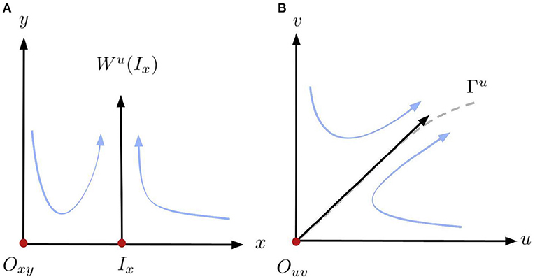
Figure 2. Diagram of the horizontal blow-up and blow-down in a neighborhood of the origin (0, 0). (A) Blow-up. (B) Blow-down.

Next, we consider the stability of the positive equilibria of system (4). Note that these equilibria are the intersection of the nullcline u = v such that (u + A)(1 − u)(u − M) = Qu. Therefore, the Jacobian matrix of system (4) becomes

$\begin{array}{ll}J(u,u)=\left(\begin{array}{cc}{u}^2((1-u)(u-M)-(u+A)& -Q{u}^2\\ (u-M)+(1-u)(u+A))\\ Su(A+u)& -Su(A+u)\end{array}\right).& (14)\end{array}$

The determinant and the trace of the Jacobian matrix (14) are:

$\begin{array}{ll}\begin{array}{l}det(J(u,u))=S{u}^2(A+u)(u^2(2u-T(A,M))-AM),\\ \text{ tr}(J(u,u))=u(((1-u)(u-M)+(u+A)(1-2u+M))\\ u-S(A+u)).\end{array}& (15)\end{array}$

So, the parity of the determinant (15) depends on the sign of u²(2u − T(A, M)) − AM and the parity of the trace (15) depends on the sign of

$\begin{array}{ll}((1-u)(u-M)+(u+A)(1-2u+M))u-S(A+u).& (16)\end{array}$

This instantly yields the following result:

Lemma 3.2. A positive equilibrium P = (ũ, ũ) of (4) will be

  (i) a saddle point if (ũ)²(2ũ − T(A, M)) − AM < 0;

 (ii) a repeller if (ũ)²(2ũ − T(A, M)) − AM > 0 and $S<\frac{\tilde{u}((1-\tilde{u})(\tilde{u}-M)+(\tilde{u}+A)(1-2\tilde{u}+M))}{(A+\tilde{u})}=:f(\tilde{u})$; and

(iii) an attractor if (ũ)²(2ũ − T(A, M)) − AM > 0 and $S>\frac{\tilde{u}((1-\tilde{u})(\tilde{u}-M)+(\tilde{u}+A)(1-2\tilde{u}+M))}{(A+\tilde{u})}$.

Corrolary 3.1. If T(A, M)³ < −27AM, then a positive equilibrium P = (ũ, ũ) of (4) is not a saddle. If for a positive equilibrium P = (ũ, ũ) we have that $\tilde{u}>T(A,M)+\sqrt{T{(A,M)}^2+3(A-M+AM)}$, then this equilibrium is not a repeller.

Proof: The first statement follows directly from the observation that (ũ)²(2ũ − T(A, M)) − AM is minimal for non-negative ũ at ũ = û: = max{0, T(A, M)/3}. At this point (ũ)²(2ũ − T(A, M)) − AM simplifies to min{−AM, −T(A, M)³/27 − AM}. Hence, (ũ)²(2ũ − T(A, M)) − AM > 0 for all ũ if T(A, M)³ < −27AM. The second statement follows directly from the observation that for $\tilde{u}>T(A,M)+\sqrt{T{(A,M)}^2+3(A-M+AM)}$ we have that f(ũ) < 0.□

In addition, f(ũ) has a maximum for positive ũ. Hence, a value for S larger than this maximum again yields that the associated equilibrium cannot be a repeller. For given A and M this maximum value can be explicitly computed. For instance, this maximum value is 361/1200 for A = 1/10 and M = −1/10.

In the case that there is only one positive equilibrium, Lemma 3.2 simplifies to the following.

Corrolary 3.2. Let the system parameters of (4) be such that the conditions of case (I) or case (II)(i) of Lemma 2.1 are met. Then, system (4) has only one positive equilibrium P = (u*, u*) which is a repeller or an attractor. If the positive equilibrium is a repeller, then it is surrounded by a stable limit cycle.

Proof: This result follows directly from the observation that Φ (9) forms a bounding box and the fact that the equilibria (0, 0) and (1, 0) are (non-hyperbolic) saddle points, see Lemma 3.1.□

Examples of Corollary 3.2 are shown in Figure 3.

FIGURE 3

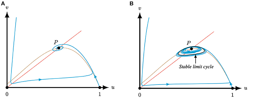
Figure 3. For A = 0.5, M = −0.05, and Q = 0.51, such that T(0.5, −0.05) > 0 and L(0.5, −0.05, 0.51) > 0, i.e., case (I) of Lemma 2.1, system (4) has one positive equilibrium P. This equilibrium can be an attractor if S = 0.1 (A) or a repeller surrounded by a limit cycle if S = 0.045 (B), see Corollary 3.2. In the latter case, the equilibrium is necessarily surrounded by a stable limit cycle. The brown (red) curve represents the predator (prey) nullcline.

In the case that there are three distinct positive equilibria, Lemma 3.2 simplifies to the following.

Corrolary 3.3. Let the system parameters of (4) be such that the conditions of case (II)(ii) of Lemma 2.1 are met. Then, system 2.1 has three positive equilibria $P_1=(u^{*},u^{*}),P_2=(u_{-}^{*},u_{-}^{*})$ and $P_3=(u_{+}^{*},u_{+}^{*})$. If the three equilibria are distinct, then the middle equilibrium is a saddle point, while the outer two equilibria are a repeller or an attractor. If both outer equilibria are repellers, then there is a stable limit cycle surrounding the equilibria.

Proof: Recall that we assumed, without loss of generality, $0<u^{*}<u_{-}^{*}<u_{+}^{*}<1$, that is, P₂ is the middle equilibrium. Now the first two results immediately follow from Lemma 3.2, the conditions of case (II)(ii) of Lemma 2.1 and the expressions for $u_{\pm }^{*}$ in terms of u* (8). In particular, for the middle equilibrium $P_2=(u_{-}^{*},u_{-}^{*})$ we have

$\begin{array}{l}{(u_{-}^{*})}^2\left(2u_{-}^{*}-T(A,M)\right)-AM\\ =\frac{\sqrt{\Delta }}{4}\left(-1-A-M+3u^{*}+\sqrt{\Delta }\right)\\ =u_{-}^{*}\sqrt{\Delta }\left(u^{*}-u_{-}^{*}\right)<0.\end{array}$

Similarly, for $P_3=(u_{+}^{*},u_{+}^{*})$ we get

$\begin{array}{l}{(u_{+}^{*})}^2\left(2u_{+}^{*}-T(A,M)\right)-AM\\ =\frac{\sqrt{\Delta }}{4}\left(-T(A,M)+3u^{*}-\sqrt{\Delta }\right)\\ =u_{+}^{*}\sqrt{\Delta }\left(u_{+}^{*}-u^{*}\right)>0.\end{array}$

To show that P₁ cannot be a saddle point, we recall that the number of equilibria as discussed in Lemma 2.1, and their stability, is independent of our initially picked root u*. Therefore, assume that initially picked root ũ* in Lemma 2.1 is the largest root (where we added the ~ to make the distinction with the previous choice). Now, $0<{\tilde{u}}_{-}^{*}<{\tilde{u}}_{+}^{*}<{\tilde{u}}^{*}<1$ and we have that

$\begin{array}{l}{({\tilde{u}}_{-}^{*})}^2\left(2{\tilde{u}}_{-}^{*}-T(A,M)\right)-AM\\ =\frac{\sqrt{\Delta }}{4}\left(-1-A-M+3{\tilde{u}}^{*}+\sqrt{\Delta }\right)\\ ={\tilde{u}}_{-}^{*}\sqrt{\Delta }\left({\tilde{u}}^{*}-{\tilde{u}}_{-}^{*}\right)>0.\end{array}$

Hence, also P₁ cannot be a saddle point.

The final statement again follows directly from the observation that Φ (9) forms a bounding box and the fact that the equilibria (0, 0) and (1, 0) are (non-hyperbolic) saddle points, see Lemma 3.1.□

Examples of Corollary 3.3 are shown in Figure 4.

FIGURE 4

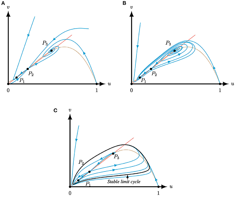
Figure 4. Phase planes of system (4) for A = 0.1, M = −0.1 and Q = 0.363, such that system (4) has three positive equilibria P, for varying S (Corollary 3.3). The equilibria (0, 0), (1, 0) and P₂ are always saddles. The brown (red) curve represents the predator (prey) nullcline. (A) For S = 0.3 the equilibria P_1,3 are attractors. (B) For S = 0.2 the equilibria P₁ is an attractor and P₃ is a repeller. (C) For S = 0.13 the equilibria P_1,3 are repellers. The equilibria are surrounded by a stable limit cycle.

To conclude, we discuss the cases when two of the equilibria collapse, see Figures 1, 5. Since we assumed, without loss of generality, that $0<u^{*}\le u_{-}^{*}\le u_{+}^{*}<1$, either $P_1=(u^{*},u^{*})$ collapses with $P_2=(u_{-}^{*},u_{-}^{*})$ or P₂ collapses with $P_3=(u_{+}^{*},u_{+}^{*})$. We obtain the following result for the colliding equilibria.

FIGURE 5

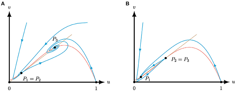
Figure 5. Phase planes of system (4) for A = 0.1, M = −0.1 and S = 0.25 for varying Q. The equilibria (0, 0) and (1, 0) are always saddles. The brown (red) curve represents the predator (prey) nullcline. (A) For $Q=Q^{-}(0.1,-0.1)=(73-\sqrt{5})/200$ the equilibria P₁ and P₂ coincide and form a stable saddle-node [Corollary 3.4(i)], while the equilibrium P₃ is an attractor [Lemma 3.2(ii)]. (B) For $Q=Q^{+}(0.1,-0.1)=(73+\sqrt{5})/200$ the equilibria P₂ and P₃ coincide and form an unstable saddle-node [Corollary 3.4(i)], while the equilibrium P₁ is an attractor [Lemma 3.2(ii)].

Corrolary 3.4. Let the system parameters of (4) be such that the conditions of case 2.12.1 of Lemma 2.1 are met.

  (I) If P₁ collides with P₂, then this equilibrium point P₁ = P₂ of multiplicity two is

(i) an unstable saddle-node if $S<\frac{Q{u}^{*}}{A+u^{*}}$,

(ii) a stable saddle-node if $S>\frac{Q{u}^{*}}{A+u^{*}}$.

(II) If P₂ collides with P₃, then this equilibrium point P₂ = P₃ of multiplicity two is

(i) an unstable saddle-node if $S<\frac{Q(T(A,M)-u^{*})}{1+A+M-u^{*}}$,

(ii) a stable saddle-node if $S>\frac{Q(T(A,M)-u^{*})}{1+A+M-u^{*}}$.

Proof: We focus on the case where P₂ collapses with P₃. The proof of the other case goes in a similar fashion and will be omitted. The equilibrium coincide when Δ = 0 (7) and $u_{-}^{*}=u_{+}^{*}=(T(A,M)-u^{*})/2$. The Jacobian matrix (14) reduces to

$\begin{array}{ll}J\left(u_{-}^{*},u_{-}^{*}\right)=\left(\begin{array}{cc}Q{\left(u_{-}^{*}\right)}^2& -Q{\left(u_{-}^{*}\right)}^2\\ S{u}_{-}^{*}\left(A+u_{-}^{*}\right)& -S{u}_{-}^{*}\left(A+u_{-}^{*}\right)\end{array}\right).& (17)\end{array}$

So, as expected, $det(J(u_{-}^{*},u_{-}^{*}))=0$ and the behavior of the equilibrium depends on the value of the trace

$\text{tr}(J(u_{-}^{*},u_{-}^{*}))=Q{(u_{-}^{*})}^2-S{u}_{-}^{*}(A+u_{-}^{*}).$

Implementing $u_{-}^{*}=(T(A,M)-u^{*})/2$ now gives the desired result. Note that since $u_{-}^{*}=u_{+}^{*}=(T(A,M)-u^{*})/2>0$ implies that T(A, M) > u*. Consequently, 1 + A + M − u* > T(A, M) − u* > 0.□

Since Equation (5) does not depend on the parameter S it does not affect the number of positive equilibria. In contrast, modifying Q impacts Δ (7) and hence the number of positive equilibria. If we assume that the system parameters are such that we have three distinct positive equilibria $P_1=(u^{*},u^{*}),P_2=(u_{-}^{*},u_{-}^{*})$ and $P_3=(u_{+}^{*},u_{+}^{*})$ with $u^{*}<u_{-}^{*}<u_{+}^{*}$, then the equilibrium P₂ is a saddle point, while the other equilibria P₁ and P₃ are repellers or attractors, see Corollary 3.3. Let $W_{\swarrow }^s(P_2)$ denote the stable manifold of P₂ that approaches P₂ from a northeast direction and $W_{\nearrow }^s(P_2)$ the stable manifold of P₂ that approaches P₂ from a southwest direction, see Figure 6A. By continuity of the vector field in S and the parameter Q fixed (see Figure 6), the following behavior is observed for the equilibria P₁ and P₃:

  (i) For large S, Lemma 3.2 yields that both P₁ and P₃ are repellers (i.e., for $S>{max}_{\tilde{u}\in (0,1)}f(\tilde{u})$, where f is defined in Lemma 3.2) and consequently we observe that $W_{\swarrow }^s(P_2)$ connects to the boundary of region Φ (9). In particular, $W^s(P_2)=W_{\nearrow }^s(P_2)\bigcup W_{\swarrow }^s(P_2)$ creates a separatrix curve between the basin of attraction of P₁ and P₃. Hence, any solutions having initial conditions above the separatrix lie in the basin of attraction of P₁, see orange region of Figure 6. Whereas, any solutions with initial conditions under of the separatrix lie in the basin of attraction of P₃, see grey region of Figure 6. The α-limit of $W_{\swarrow }^s(P_2)$ is outside of Φ, hence the curve $W_{\swarrow }^s(P_2)$ lies above $W_{\nwarrow }^u(1,0)$, the unstable manifold of (1, 0) that leaves (1, 0) in a northwest direction and necessarily remains in Φ. Hence $W_{\nwarrow }^u(1,0)$ connects to P₃, see Figure 6A.⁴

 (ii) Then, by further reducing S, there exists conditions in the (Q, S)-parameters space for which the two manifolds $W_{\nwarrow }^u(1,0)$ and $W_{\swarrow }^s(P_2)$ coincide, forming the heteroclinic curve [32], see Figure 6B.

(iii) Upon further decreasing S, $W^s(P_2)$ connects with (0, 0), see Figure 6C. Furthermore, there exists an S-value for which $W_{\swarrow }^s(P_2)$ connects with $W_{\nearrow }^u(P_2)$ (i.e., $W_{\swarrow }^s(P_2)=W_{\nearrow }^u(P_2)$) generating an homoclinic curve. Note that this case is not shown in Figure 6 but it lies between S = 0.235 of Figure 6C and S = 0.225 of Figure 6D.

(iv) When the homoclinic breaks an unstable limit cycle is created around P₂, see Figure 6D.

 (v) Upon further decrasing S, P₃ becomes unstable and P₁ turns into an attractor and $W_{\nwarrow }^u(1,0)$ connects to P₁, see Figure 6E.

(vi) Finally, if the system parameters are such that f(u*) and $f(u_{+}^{*})$ are positive, where f is defined in Lemma 3.2, then, P₁ and P₃ are repellers for $S<min\{f(u^{*}),f(u_{+}^{*})\}$. Hence, by Corollary 3.3 the system possesses a limit cycle, and $W_{\nwarrow }^u(1,0)$ connects to this limit cycle, while $W_{\swarrow }^s(P_2)$ connects with $W_{\swarrow }^u(P_3)$ and $W_{\nearrow }^s(P_2)$ connects with $W_{\nearrow }^u(P_1)$, see Figure 6F.

Note that the dynamics described above is also observed in studies related to heteroclinic cycles. These dynamics refer to heteroclinic trajectories which are saddle-type of invariant sets. For instance, in [34] the authors observed that the system could experience by continuity a saddle-node bifurcation, a Hopf bifurcation and a homoclinic bifurcation.

FIGURE 6

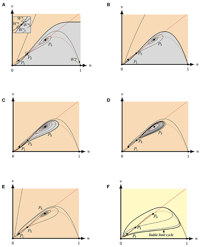
Figure 6. Phase plane of system (4) for A = 0.1, M = −0.1 and Q = 0.363 for varying S. The equilibria (0, 0), (1, 0) and P₂ are always saddles. The brown (red) curve represents the predator (prey) nullcline. (A) For S = 0.3 both P₁ and P₃ are attractors. The stable manifold of P₂ (W^s) forms a separatrix between the basin of attraction of P₁ (orange region) and the basin of attraction of P₃ (grey region) and $W_{\nwarrow }^u(1,0)$ connects to P₃. (B) For S = 0.24962827 both P₁ and P₃ are still attractors and the stable manifold of P₂ still forms a separatrix between the two basins of attraction. However, the separatrix now connects to $W_{\nwarrow }^u(1,0)$ forming a heteroclinic curve between P₂ and (1, 0). (C) For S = 0.235 both P₁ and P₃ are attractors. The stable manifold of P₂ forms a separatrix between the basin of attraction of P₁ (orange region) and the basin of attraction of P₃ (grey region). Here, $W_{\nearrow }^s(P_2)$ connects to (0, 0) and $W_{\nwarrow }^u(1,0)$ connects to P₁. (D) For S = 0.225 both P₁ and P₃ are still attractors and P₃ is surrounded by an unstable limit cycle. This limit cycle forms a separatrix between the two basins of attraction. Here, $W_{\nwarrow }^u(1,0)$ connects to P₁. (E) For S = 0.18 the equilibria P₃ is a repeller and P₁ is a global attractor. Hence, also $W_{\nwarrow }^u(1,0)$ now connects to P₁. (F) For S = 0.13 both P₁ and P₃ are repellers and $W_{\nwarrow }^u(1,0)$ connects to a stable limit cycle which surrounds the three positive equilibria.

3.2. Bifurcation Analysis

In this section, we discuss some of the potential bifurcation scenarios. For brevity, we focus only on the case where P₂ collapses with P₃. To note, similar results, but under different parameter conditions, hold for the other case (i.e., P₁ collides with P₂) and the proofs, which will be omitted, go in a similar fashion.

Theorem 3.1. Let the system parameters of (4) be such that the conditions of case (II)(ii) of Lemma 2.1 are met and assume that P₂ and P₃ coincide, i.e., Δ = 0 (7). Then, system (4) experiences a saddle-node bifurcation at the equilibrium $P_2=P_3=(u_{-}^{*},u_{-}^{*})$.

Proof: For Δ = 0 the equilibria P₂ and P₃ collapse and reduce to $(u_{-}^{*},u_{-}^{*})=(T(A,M)-u^{*})/2$ (8). The other positive equilibrium is $P_1=(u^{*},u^{*})$ with $u^{*}<u_{-}^{*}$ by assumption. So, the Jacobian matrix of the system (4) evaluated at the equilibrium $(u_{-}^{*},u_{-}^{*})$ is

$\begin{array}{c}J(u_{-}^{*},u_{-}^{*})=\left(\begin{array}{cc}\frac{Q{(u^{*}-T(A,M))}^2}{4}& -\frac{Q{(u^{*}-T(A,M))}^2}{4}\\ \frac{\begin{array}{c}S\left(1+A+M-u^{*}\right)\\ \left(u^{*}-T(A,M)\right)\end{array}}{4}& -\frac{\begin{array}{c}S\left(1+A+M-u^{*}\right)\\ \left(u^{*}-T(A,M)\right)\end{array}}{4}\end{array}\right)\end{array},$

see also (17), and $det(J(u_{-}^{*},u_{-}^{*}))=0$. Let $V={(v_1,v_2)}^T={(1,1)}^T$ be the eigenvector corresponding to the eigenvalue λ = 0 of the matrix $J(u_{-}^{*},u_{-}^{*})$. Additionally, let $U={(u_1,u_2)}^T={(S(1+A+M-u^{*})/(Q(u^{*}-T(A,M))),1)}^T$.

The dynamical system (4) in vector form is given by

$\begin{array}{ll}f(u,v;Q)=\left(\begin{array}{c}(u+A)(1-u)(u-M)-Qv\\ u-v\end{array}\right).& (18)\end{array}$

Differentiating f(u, v, Q) with respect to the bifurcation parameter Q and evaluating at P₂ gives

$f_Q(u_{-}^{*},u_{-}^{*},Q)=\left(\begin{array}{c}\frac{u^{*}-T(A,M)}{2}\\ 0\end{array}\right).$

Therefore,

$U·f_Q(u,v;Q)=\frac{S(1+A+M-u^{*})}{2Q}\ne 0.$

Next, we analyse the expression U · D²f(u, v; Q)(V, V). The latter is given by

$\begin{array}{l}{D}^{2}f(u,v;Q)(V,V)=\frac{{\partial }^{2}f(u,v;Q)}{\partial u^2}{v}_1{v}_1+\frac{{\partial }^{2}f(u,v;Q)}{\partial u\partial v}{v}_1{v}_2\\ +\frac{{\partial }^{2}f(u,v;Q)}{\partial v\partial u}{v}_2{v}_1+\frac{{\partial }^{2}f(u,v;Q)}{\partial v^2}{v}_2{v}_2\\ =\left(\begin{array}{c}-2(2+A-M)\\ 0\end{array}\right).\end{array}$

Thus,

$\begin{array}{l}U·D^{2}f(u,v;Q)(V,V)=-\frac{2S(2+A-M)(1+A+M-u^{*})}{Q(u^{*}-T(A,M))}\\ \ne 0\end{array}.$

Therefore, by Sotomayor's Theorem ([35], section 4.2, e.g) system (4) has a saddle-node bifurcation at $P_2=(u_{-}^{*},u_{-}^{*})$.□

Theorem 3.2. Let the system parameters of (4) be such that the conditions of case (II)(ii) of Lemma 2.1 are met and assume that P₂ and P₃ coincide, i.e., Δ = 0 (7), and let

$\begin{array}{ll}S=\frac{Q(u^{*}-T(A,M))}{(1+A+M-u^{*})}.& (19)\end{array}$

Then, the equilibrium point $P_2=P_3=(u_{-}^{*},u_{-}^{*})$ is a cusp point.

See [31], for a formal definition of a cusp point.

Proof: If S = Q(u* − T(A, M))/(1 + A + M − u*), then $det(J(u_{-}^{*},u_{-}^{*}))=0$ and $\mathrm{\text{tr}}(J(u_{-}^{*},u_{-}^{*}))=0$ and the Jacobian matrix of system (4) evaluated at the equilibrium $(u_{-}^{*},u_{-}^{*})$ simplifies to

$J\left(u_{-}^{*},u_{-}^{*}\right)=-\frac{1}{4}S\left(1+A+M-u^{*}\right)\left(u^{*}-T(A,M)\right)\left(\begin{array}{cc}1& -1\\ 1& -1\end{array}\right).$

Now, we find the Jordan normal form for $J(u_{-}^{*},u_{-}^{*})$. It has repeated eigenvalues and a unique eigenvector (1, 1)^T. This vector will be the first column of the matrix of transformations ϒ₄. To obtain the second column, we choose a vector that makes the matrix ϒ₄ non-singular. In this case, we take (−1, 0)^T. Thus,

${\Upsilon }_4=\left(\begin{array}{cc}1& -1\\ 1& 0\end{array}\right),$

and

$\begin{array}{l}{\Upsilon }_4^{-1}(J(u_{-}^{*},u_{-}^{*})){\Upsilon }_4\\ =\left(\begin{array}{cc}0& -\frac{1}{4}S(1+A+M-u^{*})(u^{*}-T(A,M))\\ 0& 0\end{array}\right).\end{array}$

Hence, we have that the equilibrium $(u_{-}^{*},u_{-}^{*})$ is a codimension 2 cusp point [36] for (Q, S) such that Δ = 0.□

A Bogdanov–Takens bifurcation can be obtained by following [36–38] where the authors showed that this type of bifurcation can be obtained by unfolding the system around the cusp of codimension two. In other words, if we consider a small neighborhood of the equilibrium point $P_2=P_3=(u_{-}^{*},u_{-}^{*})$ and Q and S vary near $S_0(Q_0):=Q_0(u^{*}-T(A,M))/(1+A+M-u^{*})$, then system (4) undergoes a Bogdanov–Takens bifurcation.

Luckily, nowadays, there are several computational methods to find Bogdanov–Takens points and these methods are implemented in software packages such as MATCONT [39]. Figure 7 illustrates the two Bogdanov–Takens bifurcations which were detected with MATCONT in the (Q, S)-plane for (A, M) fixed. In particular, the bifurcation curves obtained from Theorem 3.1 and 3.2 divide the (Q, S)-parameter-space into nine regions, see Figure 7. From our results we observe that for A and M fixed modifying the parameter Q impacts the number of positive equilibria of system (4). In contrast, the modification of the parameter S only changes the stability of the positive equilibria P₁ and P₃ of system (4), while the other equilibria (0, 0), (1, 0) and P₂ are always saddle points. When the parameters lie in the curve Q = Q⁻(A, M) the equilibria P₁ and P₂ collapse and we have $P_1=P_2=(u^{*},u^{*})$ and $P_3=(u_{+}^{*},u_{+}^{*})$ with $u^{*}<u_{+}^{*}$. In addition, when parameters lie in the curve Q = Q⁺(A, M) the equilibria P₂ and P₃ collapse and we have $P_1=(u^{*},u^{*})$ and $P_2=P_3=((T(A,M)-u^{*})/2,(T(A,M)-u^{*})/2)$. Along these lines we observe a saddle-node bifurcation, see Theorem 3.1. The system experiences a Bogdanov–Takens bifurcation if, in addition, S = Q(u* − T(A, M))/(1 + A + M − u*), see Theorem 3.2. When the parameters are located in Region I and VII, system (4) has one positive equilibrium which is an attractor, while when the parameters are located in Region II and VIII system (4) also has one positive equilibrium but now it is a repeller surrounded by a stable limit cycle, see Figure 3. When the parameters moved to Regions III–VI system (4) has three equilibria. In these regions P₂ is always a saddle point. In region III P₁ and P₃ are both attractors, see Figures 6A–C. Furthermore, when the parameters lie in Regions IV P₁ is an attractor and P₃ is an attractor surrounded by an unstable limit cycle, see Figure 6D. When the parameters lie in Regions V P₁ is an attractor and P₃ is a repeller, see Figure 6E. Finally, when the parameters are located in Region VI, P₁ and P₃ are both repellers and the equilibria P_1,2,3 are thus surrounded by a stable limit cycle, see Figure 6F. Note that Figure 7 only shows a partial bifurcation diagram, since there could exist a homoclinic curve which is located between the Hopf and the saddle-node curve. The homoclinic bifurcation and other types of bifurcations are not include in Figures 6, 7, however it could be observed in the transition from Figure 6C to Figure 6D for S ∈ (0.225, 0.235). In addition, the bifurcation curves observed in Figure 7 are qualitatively similar to the bifurcation studied in [34]. In particular, the authors observed that the variation of two parameters impacts the number of equilibria of the system and the stability of these equilibria. It was also observed that, by continuity, the stability of an equilibrium point changes from stable to unstable point surrounded by a stable limit cycle. Then, the limit cycle increases until it joins a homoclinic curve which is the connection between the stable and unstable manifold of a saddle point.

FIGURE 7

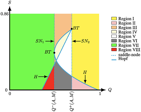
Figure 7. The bifurcation diagram of system (4) for (A, M) = (0.1, −0.1) fixed created with the numerical bifurcation package MATCONT [39]. The curve H represents the Hopf curve, SN_1,2 represents the saddle-node curve, and BT represents the Bogdanov–Takens bifurcation.

4. Conclusions

In this manuscript, we studied a Leslie–Gower predator-prey model with weak Allee effect and functional response Holling type II, i.e., system (2) with m < 0. We simplified the analysis by studying a topologically equivalent system (4). The topologically equivalent system (4) has two equilibria on the axis which are always (non-hyperbolic) saddle points, see Lemma 3.1. In addition, system (4) has at most three positive equilibria in the first quadrant, see Lemma 2.1 and Figure 1. As the function φ is a diffeomorphism preserving the orientation of time, the dynamics of system (2) is topologically equivalent to system (4) ([29], Theorem 1). Therefore, we can, for instance, conclude from the results of section 3 that there are conditions on the system parameter for which the predator and prey can coexist without oscillations or with oscillations, see Figure 6 and this behavior depends intrinsically and non-linearly on the system parameters including the predation rate (q) and the intrinsic growth rate of the predator (s).

In more detail, when the system parameters are such that system (4) has only one positive equilibrium, i.e., Q < Q⁻(A, M) or Q > Q⁺(A, M), see Regions I, II, VII and VIII in Figure 7, then it is a repeller surrounded by a stable limit cycle or an attractor, but not a saddle point, see Corollary 3.2 and Figure 3. Note that when the equilibrium is an attractor it is not necessary a global attractor since there is a small region in parameter space near the Hopf bifurcation where the equilibrium is surrounded by two limit cycles, see Figure 8A. The observed behavior for system (4), and hence system (2) with m < 0, in this case of one positive equilibrium – global attractor, attractor with two limit cycles, or repeller with one limit cycle – is similar to the behavior of the original Leslie–Gower predator-prey (1) with logistic growth for the prey [40]. In other words, for q smaller than some q⁻ or larger than some q⁺ both systems (1) and (2) with m < 0 present qualitatively similar behaviors, see Figure 3B.

FIGURE 8

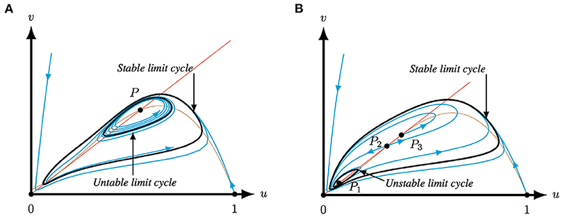
Figure 8. Phase plane of system (4) for A = 0.1 and M = −0.1 for varying Q and S. The equilibria (0, 0) and (1, 0) are always saddles. The brown (red) curve represents the predator (prey) nullcline. (A) For Q = 0.345 and S = 0.134332 P₁ is an attractor surrounded by two limit cycles, the inner one is unstable, while the outer limit cycle is stable. (B) For for Q = 0.363 and S = 0.1298 system (4) has three equilibria. Here, P₂ is a saddle, P₁ is an attractor surrounded by an unstable limit cycles and P₃ is a repeller. The three positive equilibria P_1,2,3 are surrounded by a stable limit cycle.

In contrast, for Q⁻(A, M) < Q < Q⁺(A, M), system (4) has three equilibria in the first quadrant, which is not possible in the original Leslie–Gower predator-prey (1) nor in the model with strong Allee effect, i.e., system (2) with m > 0. In this case, the middle one is always a saddle point, while the outer two are repellers or attracters, see Corollary 3.3 and Figures 4, 6. If the two outer equilibria are attractors, then either the stable manifold of the saddle point determines a separatrix curve which divides the basins of attraction of the two attracters, or there exists an unstable limit cycle dividing the basins of attraction, see Figures 6A–D. When both outer equilibria are repellers the system necessarily possesses a stable limit cycle, see Figure 6F. When the outer equilibria are an attractor and a repeller, the attractor can be a global attractor or there are two limit cycles surrounding the equilibria, see Figures 6E, 8B. The latter one again happens near the Hopf bifurcation. In other words, there are regions in parameter space for which system (4) has two attractors or an attractor and a stable limit cycle. As such, a modification of one, or both, of the species could have the result that you end up in a different basin of attraction and you will thus have significantly different dynamics as you will approach the other attractor, see Figures 6A–D, 8B. We also performed an initial (numerical) bifurcation analysis which revealed the existence of saddle-node and Bogdanov–Takens bifurcations, see Theorems 3.1 and 3.2 and Figure 7.

In summary, we showed that the weak Allee effect in the Leslie–Gower model (2) presents—due to the presence of a region in parameter space where we have three positive equilibria—richer dynamics than the original Leslie–Gower predator-prey model (2) studied, for example, by Saez and Gonzalez-Olivares [40]. The original Leslie–Gower predator-prey model (2) does not possess the bifurcations studied in section 3.2. That is, a saddle-node bifurcation and a Bogdanov–Takens bifurcation. Moreover, the original model only has one positive equilibrium point, which can be stable surrounded by two limit cycles. Therefore, the populations could switch between a stable state or an oscillatory behavior. However, system (2) with a weak Allee effect can have two stable equilibria and thus depending on the initial condition the population could end up in two stable states. From an ecological point of view, we can also conclude that the species in system (2) could coexist or oscillate but never go extinct, see Figure 6. This behavior was also observed by Ostfeld and Canhan [24]. The authors found that the stabilization of vole (Microtus agrestis) populations in Southeastern New York depend on the variation in reproductive rate and thus this impact the reproductive activity of the species. This is again similar to the original Leslie–Gower predator-prey model (2), but different from the Leslie–Gower model (2) with strong Allee effect, i.e., m > 0. In the latter case, the model supports coexistence and extinction of the species [29].

Data Availability Statement

The original contributions presented in the study are included in the article/supplementary material, further inquiries can be directed to the corresponding author/s.

Author Contributions

CA-I implemented the methodology, performed the analytics and numerical analysis, composed all the figures, drafted the manuscript, wrote the cover letter and acted as the corresponding author. JF provided the technical assistance with the interpretation of the results and critically reviewed the manuscript. PH directed the research, provided the technical assistance with the interpretation of the results and critically reviewed the manuscript. All authors contributed to the article and approved the submitted version.

Conflict of Interest

The authors declare that the research was conducted in the absence of any commercial or financial relationships that could be construed as a potential conflict of interest.

Publisher's Note

All claims expressed in this article are solely those of the authors and do not necessarily represent those of their affiliated organizations, or those of the publisher, the editors and the reviewers. Any product that may be evaluated in this article, or claim that may be made by its manufacturer, is not guaranteed or endorsed by the publisher.

Footnotes

1. ^We will refer to equilibria with two positive entries as positive equilibria.

2. ^Note that (2) is singular along N = 0, and the equilibria (0, 0) is thus also a singular point in (2) with m < 0.

3. ^The same expressions for Q^± are obtained when we compute two other roots coincide.

4. ^A priori, the role of P₁ and P₃ could be interchanged.

References

1. Arancibia-Ibarra C. The basins of attraction in a modified May-Holling-Tanner predator-prey model with Allee effect. Nonlinear Anal Theory Methods Appl. (2019) 185:15–28. doi: 10.1016/j.na.2019.03.004

CrossRef Full Text | Google Scholar

2. Kundu S, Maitra S. Asymptotic behaviors of a two prey one predator model with cooperation among the prey species in a stochastic environment. J Appl Math Comput. (2019) 61:505–31. doi: 10.1007/s12190-019-01251-4

CrossRef Full Text | Google Scholar

3. Martínez-Jeraldo N, Aguirre P. Allee effect acting on the prey species in a Leslie–Gower predation model. Nonlinear Anal Real World Appl. (2019) 45:895–917. doi: 10.1016/j.nonrwa.2018.08.009

CrossRef Full Text | Google Scholar

4. Mateo R, Gastón A, Aroca-Fernández M, Broennimann O, Guisan A, Saura A, et al. Hierarchical species distribution models in support of vegetation conservation at the landscape scale. J Veget Sci. (2019) 30:386–96. doi: 10.1111/jvs.12726

PubMed Abstract | CrossRef Full Text | Google Scholar

5. Mondal A, Pal A, Samanta GP. On the dynamics of evolutionary Leslie-Gower predator-prey eco-epidemiological model with disease in predator. Ecol Genet Genomics. (2019) 10:1–12. doi: 10.1016/j.egg.2018.11.002

CrossRef Full Text | Google Scholar

6. Santos X, Cheylan M. Taxonomic and functional response of a Mediterranean reptile assemblage to a repeated fire regime. Biol Conserv. (2013) 168:90–98. doi: 10.1016/j.biocon.2013.09.008

CrossRef Full Text | Google Scholar

7. Turchin P. Complex Population Dynamics: A Theoretical/Empirical Synthesis. Princeton, NJ: Princeton University Press (2003).

Google Scholar

8. Hooper D, Chapin F, Ewel J, Hector A, Inchausti P, Lavorel S, et al. Effects of biodiversity on ecosystem functioning: a consensus of current knowledge. Ecol Monogr. (2005) 75:3–35. doi: 10.1890/04-0922

PubMed Abstract | CrossRef Full Text | Google Scholar

9. May R. Stability and Complexity in Model Ecosystems. Princeton, NJ: Princeton University Press (1974).

Google Scholar

10. Moller AP, Stokke BG, Samia DSM. Hawk models, Hawk mimics, and antipredator behavior of prey. Behav Ecol. (2015) 26:1039–44. doi: 10.1093/beheco/arv043

CrossRef Full Text | Google Scholar

11. Monclus R, von Holst D, Blumstein D, Rödel H. Long-term effects of litter sex ratio on female reproduction in two iteroparous mammals. Funct Ecol. (2014) 28:954–62. doi: 10.1111/1365-2435.12231

CrossRef Full Text | Google Scholar

12. Hanski I, Henttonen H, Korpimäki E, Oksanen L, Turchin P. Small–rodent dynamics and predation. Ecology. (2001) 82:1505–20. doi: 10.1890/0012-9658(2001)082[1505:SRDAP]2.0.CO;2

CrossRef Full Text | Google Scholar

13. Hanski I, Hansson L, Henttonen H. Specialist predators, generalist predators, and the microtine rodent cycle. J Anim Ecol. (1991) 60:353–67. doi: 10.2307/5465

CrossRef Full Text | Google Scholar

14. Roux P, Shaw J, Chown S. Ontogenetic shifts in plant interactions vary with environmental severity and affect population structure. N Phytol. (2013) 200:241–50. doi: 10.1111/nph.12349

PubMed Abstract | CrossRef Full Text | Google Scholar

15. Bimler M, Stouffer D, Lai H, Mayfield M. Accurate predictions of coexistence in natural systems require the inclusion of facilitative interactions and environmental dependency. J Ecol. (2018) 106:1839–52. doi: 10.1111/1365-2745.13030

CrossRef Full Text | Google Scholar

16. Wood S, Thomas M. Super–sensitivity to structure in biological models. Proc R Soc Lond Ser B Biol Sci. (1999) 266:565–70. doi: 10.1098/rspb.1999.0673

CrossRef Full Text | Google Scholar

17. Graham IM, Lambin X. The impact of weasel predation on cyclic field-vole survival: the specialist predator hypothesis contradicted. J Anim Ecol. (2002) 71:946–56. doi: 10.1046/j.1365-2656.2002.00657.x

CrossRef Full Text | Google Scholar

18. Leslie P. Some further notes on the use of matrices in population mathematics. Biometrika. (1948) 35:213–45. doi: 10.1093/biomet/35.3-4.213

PubMed Abstract | CrossRef Full Text | Google Scholar

19. Courchamp F, Clutton-Brock T, Grenfell B. Inverse density dependence and the Allee effect. Trends Ecol Evol. (1999) 14:405–10. doi: 10.1016/S0169-5347(99)01683-3

PubMed Abstract | CrossRef Full Text | Google Scholar

20. Courchamp F, Berec L, Gascoigne J. Allee effects in Ecology and Conservation. Oxford University Press (2008).

Google Scholar

21. Stephens P, Sutherland W. Consequences of the Allee effect for behaviour, ecology and conservation. Trends Ecol Evol. (1999) 14:401–5.

PubMed Abstract | Google Scholar

22. Allee W, Park O, Emerson A, Park T, Schmidt K. Principles of Animal Ecology. Philadelphia, PA: WB Saundere Co. Ltd. (1949).

Google Scholar

23. Berec L, Angulo E, Courchamp F. Multiple Allee effects and population management. Trends Ecol Evol. (2007) 22:185–91. doi: 10.1016/j.tree.2006.12.002

PubMed Abstract | CrossRef Full Text | Google Scholar

24. Ostfeld R, Canham C. Density-dependent processes in meadow voles: an experimental approach. Ecology. (1995) 76:521–32.

Google Scholar

25. Arancibia-Ibarra C, González-Olivares E. A modified Leslie–Gower predator–prey model with hyperbolic functional response and Allee effect on prey. In: BIOMAT 2010 International Symposium on Mathematical and Computational Biology. Rio de Janeiro (2011). p. 146–62.

Google Scholar

26. González-Olivares E, Gallego-Berrío L, González-Yañez B, Rojas-Palma A. Consequences of weak Allee effect on prey in the May–Holling–Tanner predator–prey model. Math Methods Appl Sci. (2015) 38:5183–6. doi: 10.1002/mma.3441

PubMed Abstract | CrossRef Full Text | Google Scholar

27. González-Olivares E, Mena-Lorca J, Rojas-Palma A, Flores J. Dynamical complexities in the Leslie–Gower predator–prey model as consequences of the Allee effect on prey. Appl Math Modell. (2011) 35:366–81. doi: 10.1016/j.apm.2010.07.001

CrossRef Full Text | Google Scholar

28. Tintinago-Ruíz P, Restrepo-Alape L, González-Olivares E. Consequences of weak Allee effect in a Leslie–Gower-type predator–prey model with a generalized holling type III functional response. In: Analysis, Modelling, Optimization, and Numerical Techniques. Denmark: Springer (2015). p. 89–103.

Google Scholar

29. Arancibia-Ibarra C, Flores J, Pettet G, van Heijster P. A Holling–Tanner predator–prey model with strong Allee effect. Int J Bifurc Chaos (2019) 29:1–16. doi: 10.1142/S0218127419300325

CrossRef Full Text | Google Scholar

30. Dumortier F, Llibre J, Artés J. Qualitative Theory of Planar Differential Systems. Berlin; Heidelberg: Springer-Verlag (2006).

Google Scholar

31. Andronov A. Qualitative Theory of Second-Order Dynamic Systems. Halsted Press (1973).

32. Chicone C. Ordinary Differential Equations with Applications. Berlin: Springer Science & Business Media (2006).

Google Scholar

33. Curtiss D. Recent extensions of Descartes' rule of signs. Ann Math. (1918) 19:251–78.

Google Scholar

34. Labouriau I, Rodrigues A. Bifurcations from an attracting heteroclinic cycle under periodic forcing. J Diff Equat. (2020) 269:4137–74. doi: 10.1016/j.jde.2020.03.024

CrossRef Full Text | Google Scholar

35. Perko L. Differential Equations and Dynamical Systems. New York, NY: Springer (2001).

36. Xiao D, Ruan S. Bogdanov–Takens bifurcations in predator–prey systems with constant rate harvesting. Fields Inst Commun. (1999) 21:493–506.

37. Huang J, Gong Y, Ruan S. Bifurcation analysis in a predator-prey model with constant-yield predator harvesting. Discrete Contin Dyn Syst Ser B. (2013) 18:2101–21. doi: 10.3934/dcdsb.2013.18.2101

CrossRef Full Text | Google Scholar

38. Zhu C, Lan K. Phase portraits, Hopf bifurcations and limit cycles of Leslie-Gower predator-prey systems with harvesting rates. Discrete Contin Dyn Syst B. (2010) 14:289. doi: 10.3934/dcdsb.2010.14.289

CrossRef Full Text | Google Scholar

39. Dhooge A, Govaerts W, Kuznetsov Y. Matcont: a matlab package for numerical bifurcation analysis of odes. ACM Trans Math Softw. (2003) 29:141–164. doi: 10.1145/779359.779362

CrossRef Full Text | Google Scholar

40. Sáez E, González-Olivares E. Dynamics on a predator–prey model. SIAM J Appl Math. (1999) 59:1867–78.

Google Scholar