On Rayleigh-Taylor and Richtmyer-Meshkov Dynamics With Inverse-Quadratic Power-Law Acceleration

1 Introduction

Rayleigh-Taylor (RT) and Richtmyer-Meshkov (RM) instabilities and RT/RM interfacial mixing are fluid dynamics phenomena controlling a broad range of processes in nature and technology, at celestial and at molecular scales, in high and in low energy density regimes [1–6]. Examples include the abundance of chemical elements in supernova remnants, the magneto-spherical structure of Jupiter and Saturn, the coastal up-welling along the eastern boundary of oceans, the formation of hot spots in inertial confinement fusion, material transformations under high strain rates, nano-fabrication, and fossil fuel extraction [5–15]. RT/RM instabilities develop when fluids of different densities are accelerated against their density gradients [1–4]. The case of constant acceleration is referred as classical RT instability (RTI), whereas the case of shock induced impulsive acceleration is referred as classical Richtmyer-Meshkov instability (RMI) [1–4, 6]. In realistic environments, accelerations are often variable and are power-law functions of time [8–18]. In the work we present the first detailed investigation of RTI/RMI induced by an acceleration being an inverse-quadratic power-law function of time in a three-dimensional flow. We apply group theory to find solutions for the early-time linear and the late-time nonlinear scale-dependent RT/RM dynamics, explore properties of RT-to-RM transition, compare with existing observations achieving good agreement, and elaborate theory benchmarks for future experiments and simulations.

RT/RM flows, while occurring in vastly different physical circumstances, have similar features of their evolution [6–8, 17–19]. The instabilities start to develop when the fluid interface (and/or the flow fields) is (are) slightly perturbed near the equilibrium state. With time, the interface is transformed to a composition of a large-scale structure and small-scale structures [1–4, 6–8]. The large-scale structure consists of bubbles and spikes, with a bubble (spike) being a portion of the light (heavy) fluid penetrating the heavy (light) fluid; it’s dynamics is coherent and depends on deterministic initial conditions [1–4, 6–8, 18, 19]. Small-scale vortical structures are produced by the interfacial shear and Kelvin-Helmoholtz instability; their dynamics can be irregular [6–8, 17–19]. As time evolves, the interaction of scales enhances and the flow transitions to a stage of intense interfacial mixing [6–8]. The mixing is believed to be scale-invariant, with the amplitude of the interface perturbation increasing self-similarly in time [18]. Note that in shock-induced RM flows, the interfacial dynamics is superposed with the background motion of the fluids, and with the appearance of small-scale non-uniform structures in the bulk, including, e.g., cumulative jets, hot and cold spots, high and low pressure regions [8, 20]. While, depending on the flow Mach and Atwood numbers and the adiabatic indexes of the fluids, the background motion can be sub/super/hyper-sonic, the interfacial dynamics is usually sub-sonic and is nearly incompressible in a broad range of parameters and conditions [8, 20–22].

Non-equilibrium RT/RM dynamics is challenging to study [5–8, 17–19]. In experiment, the challenges are due to the sensitive and transient character of RTI/RMI, and the unusually tight requirements on the flow implementation and control [23–28]. Simulations must accurately track interfaces and capture small-scale processes, as well as apply highly accurate methods, massive computations and a large span of spatial and temporal scales [29–33]. In theory, one has to capture the multi-scale, nonlinear and non-local dynamics, identify universal properties of asymptotic solutions, and find symmetries and order in the unstable RT/RM flows [6–8, 34–41]. Remarkable success has recently been achieved in the understanding of the fundamentals of RTI/RMI and of RT/RM mixing [6–8]. Particularly, group theory has enabled the systematic study of RTI/RMI and RT/RM mixing and explained experimental observations in a broad range of parameters and conditions [6–8, 18, 23–28].

Having been formulated in mid-1990s, group theory approach identifies key properties of RT/RM unstable interfaces, establishes invariant measures and coherence of RT/RM dynamics, and provides with bias-free interpretations of experiments and simulations [6–8, 18, 23–28, 42, 43]. For instance, for the classical RT/RM dynamics, group theory finds that three-dimensional RT/RM flows keep isotropy in the plane normal to the acceleration, the dimensional crossover is discontinuous, and the nonlinear dynamics is essentially interfacial and multi-scale [6, 43]. While in the linear regime RT/RM dynamics is uniquely defined by the length-scale of the initial perturbation, the nonlinear RT/RM solutions both form continuous families with the number of the family parameters set by flow symmetries [42–44]. Yet, the shape of nonlinear RT bubble is curved because it moves steady, and that of RM bubble is flattened because it decelerates. These results achieved excellent agreement with experiments and simulations [6, 7, 18, 20, 24, 43–45]. Group theory approach further finds that the invariant, correlation, scaling and spectral properties of RT mixing depart substantially from those of canonical turbulence, and that RT mixing with constant acceleration keeps order even at high Reynolds numbers, $\sim 3.2\mathrm{x}10^6$. This explained the experiments in fluids and plasmas [6–8, 18, 23, 24, 27, 28].

Some important aspects of RT/RM dynamics still require better understanding [8]. One such aspect is the link between RT and RM dynamics [8, 18]. In applications, this aspect is critical for blast-wave-driven RTI/RMI in core-collapse supernovae, for RT/RM unstable plasma irregularities in the Earth’s ionosphere, for RTI/RMI induced by unsteady shocks in inertial confinement fusion, and for RT/RM instabilities in the fossil fuel industry [8–15]. As regards to fundamentals, since classical RTI is driven by the acceleration and classical RMI is driven by the initial growth-rate dependent on the initial conditions, the link between RT and RM dynamics can be self-consistently revealed for variable accelerations, particularly, for accelerations whose magnitudes vary as power-laws in time [8, 46–49]. Power-law functions are important to consider because they can yield special invariant and scaling properties of RT/RM dynamics, and can also be used to adjust the acceleration’s time-dependence in applications [8, 46–49].

By applying group theory approach, recent research on RTI/RMI with variable acceleration, which has magnitude g = Gt^a with G, a being respectively the acceleration’s strength and exponent, found the dependence of RTI/RMI dynamics on the exponent a of the acceleration’s power-law [8, 46–49] The linear and nonlinear interfacial dynamics is of RT type and is driven by the acceleration with magnitude g = Gt^a for the acceleration exponents greater than negative two, a >−2 [8, 46–49]. It is of RM type and is driven by the initial growth rate with magnitude v₀ for the acceleration exponents smaller than negative 2, a <−2. The properties of the scale-dependent RT and RM dynamics differ substabtially from one another in both the linear or nonlinear regimes [8, 46–49]. Detailed investigation is thus required of RT/RM dynamics and RT-to-RM transition at the acceleration exponent equal to negative two, a =−2 [8].

To illustrate the importance of the acceleration exponent a =−2 physically and mathematically, we recall that for a given value of the length scale λ, which is the wavelength of the initial perturbation, the acceleration strength G and the initial growth-rate v₀ establish the characteristic time scales τ_G ∼ (λ/G)^1/(a+2) and τ₀ ∼ λ/v₀. For a >−2 the time scales relate as τ_G ≪ τ₀, and the fastest process is set by the acceleration. For a <−2 the time scales relate as τ₀ ≪ τ_G, and the fastest process is set by the initial growth-rate. At a =−2, the acceleration strength G has the dimension of the length scale λ, and the interplay of length scales G and λ defines properties of RT-to-RM transition [8].

Here we study RTI and RMI induced by variable acceleration with inverse-quadratic power-law time dependence [8, 49]. We consider a three-dimensional spatially extended periodic flow, apply group theory and scaling analysis, and identify the dependence of the linear and nonlinear dynamics of RT/RM bubbles and spikes on the acceleration’s parameters and initial conditions. In particular, we investigate the dependence of RT-to-RM transition on the acceleration strength and the fluid density ratio for both linear and nonlinear dynamics, and elaborate extensive theory benchmarks for future research.

2 Methods

2.1 Governing Equations

The dynamics of an ideal fluid is governed by the laws of conservation of mass, momentum and energy:

$\frac{\partial \rho }{\partial t}+\frac{\partial }{\partial x_i}\left(\rho v_i\right)=0,\frac{\partial }{\partial t}\left(\rho v_i\right)+\frac{\partial }{\partial x_j}\left(\rho v_i{v}_j\right)+\frac{\partial P}{\partial x_i}=0,\frac{\partial E}{\partial t}+\frac{\partial }{\partial x_i}\left(\left(E+P\right)v_i\right)=0,(1)$

where i = 1, 2, 3, (x₁, x₂, x₃) = (x, y, z) are Cartesian coordinates, t is time, ρ is its density, v its velocity, P is the pressure field and E = ρ (e + v²/2) is the energy density field, in which e is the specific internal energy [40]. The governing equations Eq. 1 are augmented with the closure equation of state associating pressure P and internal energy e [17]. We presume the equation of state has the form P = sρe with some constant s, describing an ideal fluid behaving similarly to an ideal gas [17].

There is zero mass flux across the interface, and the fluxes of mass, momentum and energy are conserved at that interface. Consequently, the boundary conditions at the interface are

$\left[\mathbf{v}\cdot \mathbf{n}\right]=0,\left[P\right]=0,\left[\mathbf{v}\cdot \mathit{\tau }\right]=\mathrm{a}\mathrm{r}\mathrm{b}\mathrm{i}\mathrm{t}\mathrm{r}\mathrm{a}\mathrm{r}\mathrm{y},\left[W\right]=\mathrm{a}\mathrm{r}\mathrm{b}\mathrm{i}\mathrm{t}\mathrm{r}\mathrm{a}\mathrm{r}\mathrm{y},(2)$

where […] is used to denote the difference in function values across the interface; the unit normal and tangent vectors at the interface are n and τ, specifically, n = ∇θ/|∇∇θ| and n ⋅ τ = 0, where θ = θ (x, y, z, t) is such that θ = 0 at the interface, θ > 0 in the bulk of the heavy fluid and θ < 0 in the bulk of the light fluid; W is the specific enthalpy W = e + P/ρ.

The heavier fluid is assumed to sit above the lighter and both are subject to a body force and a time-dependent acceleration, which is directed from the heavy fluid to the light. This acceleration influences the pressure field. The acceleration direction is chosen to be that of the z-coordinate. The acceleration g = (0, 0,−g) is such that g = Gt^a, where a is the acceleration’s power-law exponent and G > 0 is its strength. We note that G has dimensions ms^−(a+2) and a is dimensionless. The time t > t₀ > 0 where t₀ is some initial instant of time.

It is assumed that the upper and lower boundaries of the domain do not influence the dynamics and also that there is an absence of mass sources. The upper and lower boundary conditions are

$\underset{z\to \infty }{\lim }{\mathbf{v}}_h=\mathbf{0},\underset{z\to -\infty }{\lim }{\mathbf{v}}_l=\mathbf{0}.(3)$

where h indicates the heavy fluid and l indicates the light fluid. The governing equations are subject to a set of initial conditions which include the perturbations of the interface and/or the flow fields. The initial conditions define the characteristic length scale, time scale, and symmetry of the resulting flow.

2.2 Group-Theory Approach

The large-scale coherent structures in the destabilised flow are periodic arrays of bubbles and spikes in the plane normal to the acceleration direction as is set by the initial conditions. As a specific example, we consider the flow which has square symmetry [8, 41] in the plane normal to the acceleration, with wavelength λ and wavevector k = 2π/λ.

The group theory approach [6, 8, 19, 40, 41, 48, 49] accurately describes both the linear and nonlinear dynamics of the unstable interface and can be used to identify similarities and differences in the dynamics of these flows. In particularly, for linear RTI and RMI with time-varying acceleration, the linear dynamics is single-scale and is defined by the spatial period of the coherent structure, whereas the process of formation of bubbles and spikes is set by the initial conditions. For nonlinear RTI with constant and time-varying accelerations and for RMI with impulsive and time-varying accelerations, there are families of regular asymptotic solutions with the number of relevant parameters defined by the flow symmetry; the dynamics is multi-scale and characterised by the contributions of two macroscopic length scales, these being the spatial period and the amplitude of the interfacial coherent structure. Furthermore, non-equilibrium dynamics is essentially interfacial, consisting of intense fluid motion near the interface and insignificant fluid motion away from it.

Here we consider dynamics of ideal fluids, which are inviscid and are free from thermal heat flux, Eq. 1 [17]. Their velocity field is irrotational in the bulk [17, 50]. The latter can be illustrated by the analysis of slight perturbations of the fluid system in Eq. 1 near the state of hydrostatic equilibrium, similarly to [50]. Particularly: 1) by introducing a small velocity field to an initially stationary system, 2) by representing the velocity field as a superposition of a gradient of a scalar potential and a curl of a vortical potential, and 3) by considering the associated changes in the fields of density and pressure, one can linearize the system of the governing equations in the bulk Eq. 1 and the equation of state near the equilibrium state. By finding the fundamental solutions for the linear system, including their eigenvalues and eigenvectors, one can further identify the structure of the perturbation waves [50].

According to the analysis, for both compressible and incompressible ideal inviscid fluids, the vortical component of the velocity is zero in the bulk [50]. This suggests that for ideal inviscid fluids Eq. (1), the velocity field is potential in the bulk, and the vortical structures can emerge only at the interface, due to discontinuities of the tangential component of velocity and enthalpy Eq. 2. In the limit of a small viscosity, the small-scale vortical structures at the interface may be influenced by the viscosity, and the vortical structures may also appear in the bulk. However, given the interfacial character of RT/RM dynamics, the influence of the viscosity on the bulk motion may also be negligible. In this work we consider ideal incompressible fluids and their three-dimensional dynamics. We focus on RTI/RMI driven by variable accelerations with inverse quadratic power-law time-dependence and on RT-to-RM transition. We address to the future the detailed analysis of compressible and viscous effects on RT/RM dynamics.

We emphasize that even for ideal incompressible fluids, with $\dot{e}=0$ and ∇e = 0, the system (Eqs 1–3) is extremely challenging, requiring the solution of a system of nonlinear partial differential equations in a bulk, the solution of the boundary value problem at the nonlinear unstable interface, in addition to the solution of the relevant initial value problem, which is ill-posed [6, 8, 17, 19]. It is remarkably that even with this amount of complexity, the dynamics nevertheless has features of universality and order and can thus be approached using group theory [6, 19].

2.3 Dynamical System

We focus on bubbles and spikes moving in the z-direction and for convenience work in a frame of reference which moves with velocity v (t) in the z-direction, where v (t) = ∂z₀/∂t and z₀ is the position of the bubble or spike in the laboratory frame. We define the function θ (x, y, z, t) as θ (x, y, z, t) = z* (x, y, t)−z, where z = z* (x, y, t) describes the interface.

The fluids are assumed to be incompressible and stratification and density variation are negligible. We focus on large-scale coherent dynamics having length scale λ, and presume that the length scale of shear-driven interfacial vortical structures is comparatively small, ≪ λ. The fluid motion in the bulk is potential. Consequently, the velocity of the heavy fluid v_h = ∇Φ_h and that of the light fluid v_l = ∇Φ_l and the equation of conservation of mass means that Laplace’s equation ΔΦ_h(l) = 0 is satisfied in the respective bulks, that is, θ > 0 (θ < 0).

In the moving frame of reference, the interface conditions are

${\rho }_h\left(\nabla {\mathrm{\Phi }}_h\cdot \widehat{\mathbf{n}}+\frac{\dot{\theta }}{|\nabla \theta |}\right)=0={\rho }_l\left(\nabla {\mathrm{\Phi }}_l\cdot \widehat{\mathbf{n}}+\frac{\dot{\theta }}{|\nabla \theta |}\right),$

${\rho }_h\left(\frac{\partial {\mathrm{\Phi }}_h}{\partial t}+\frac{|\nabla {\mathrm{\Phi }}_h{|}^2}{2}+\left(g\left(t\right)+\frac{dv}{dt}\right)z\right)={\rho }_l\left(\frac{\partial {\mathrm{\Phi }}_l}{\partial t}+\frac{|\nabla {\mathrm{\Phi }}_l{|}^2}{2}+\left(g\left(t\right)+\frac{dv}{dt}\right)z\right),(4)$

and the vertical far-field boundary conditions are

$\frac{\partial {\mathrm{\Phi }}_h}{\partial z}{{|}_{z\to \infty }=-v\left(t\right),\frac{\partial {\mathrm{\Phi }}_l}{\partial z}|}_{z\to -\infty }=-v\left(t\right).(5)$

The periodic nature of the large-scale coherent structure can be address by means of group theory [6]. Upon identification of a group which enables structurally stable dynamics, a specific Fourier series (an irreducible representation of that group) can be employed to solve the nonlinear boundary value problem (Eqs 4, 5) For three-dimensional flow with square symmetry the potentials are [41].

${\mathrm{\Phi }}_h\left(x,y,z,t\right)=\sum _{m,n=0}^{\infty }{\mathrm{\Phi }}_{mn}\left(t\right)\left(\frac{\cos \left(mkx\right)\cos \left(nky\right)e^{-{\alpha }_{mn}kz}}{{\alpha }_{mn}k}+z\right)+f_h\left(t\right),$

${\mathrm{\Phi }}_l\left(x,y,z,t\right)=\sum _{m,n=0}^{\infty }{\tilde{\mathrm{\Phi }}}_{mn}\left(t\right)\left(\frac{\cos \left(mkx\right)\cos \left(nky\right)e^{{\alpha }_{mn}kz}}{{\alpha }_{mn}k}-z\right)+f_l\left(t\right),(6)$

where ${\alpha }_{mn}=\sqrt{m^2+n^2}$, m and n are integers, k = 2π/λ is the wavenumber, Φ_mn and ${\tilde{\mathrm{\Phi }}}_{mn}$ are the Fourier amplitudes for the heavy and light fluids respectively, with Φ₀₀ ≡ 0, ${\tilde{\mathrm{\Phi }}}_{00}\equiv 0$, and f_h (t) and f_l (t) are time-dependent functions. Symmetry requires that Φ_mn = Φ_nm and ${\tilde{\mathrm{\Phi }}}_{mn}={\tilde{\mathrm{\Phi }}}_{nm}$.

In the vicinity of the tip of a bubble or spike we make expansions in terms of the spatial coordinates. This reduces the set of governing equations to a system of oridonary differential equations (ODEs) in terms of the interface variables and the moments [6–8, 19, 40, 41].

The local behaviour of the interfacial dynamics in the vicinity of the tip of a bubble or spike can be investigated by expanding the interface function in a power series about (x, y) = (0, 0), this being

$z^{*}\left(x,y,t\right)=\sum _{N=1}^{\infty }\sum _{i+j=1}^N{\zeta }_{ij}\left(t\right)x^{2i}{y}^{2j},(7)$

where ζ_ij (t) = ζ_ji (t) due to symmetry, ζ (t) = ζ₁₀(t) is the principal curvature at the tip, and N is the order of the approximation. To lowest order (that is, N = 1), the interface is z* (x, y, t) = ζ (t) (x² + y²). Note that ζ (t) < 0, v (t) > 0 for bubbles, and ζ (t) > 0, v (t) < 0 for spikes.

The Fourier series and interface functions are substituted into the boundary conditions at the interface and the these expressions are then expanded in power series, yielding an infinite system of ordinary differential equations for Φ_mn(t), ${\tilde{\mathrm{\Phi }}}_{mn}(t)$ and ζ_ij (t).

We introduce the following moments for the heavy and light fluids:

$M_{a,b,c}\left(t\right)=\sum _{mn}{\mathrm{\Phi }}_{mn}\left(t\right){\left(mk\right)}^a{\left(nk\right)}^b{\left({\alpha }_{mn}k\right)}^c,{\tilde{M}}_{a,b,c}\left(t\right)=\sum _{mn}{\tilde{\mathrm{\Phi }}}_{mn}\left(t\right){\left(mk\right)}^a{\left(nk\right)}^b{\left({\alpha }_{mn}k\right)}^c(8)$

These are weighted sums of the (infinite number of) Fourier amplitudes. We note that M_{a, b, c} = M_{b, a, c} and M_{a+2, b, c} + M_{a, b+2, c} = M_{a, b, c+2}, by symmetry, and similarly for $\tilde{M}$. At N = 1, the series is abbreviated to second order in x, y and first order in z, since z* (x, y, t) is quadratic in both x and y.

We also define a shear function at the interface. Traditionally, in viscous fluids, such as boundary layers, the velocity share is quantified with the shear rate, which is the rate of change of velocity at which one layer of fluid passes over an adjacent layer [51]. The velocity change is caused by, e.g., the fluid’s viscosity, and the velocity shear rate is estimated in the direction normal to the direction of motion [17]. This traditional definition has a limited applicability in our problem, because in RT/RM dynamics the shear is produced by the finite jump(s) of tangential component of velocity (and enthalpy) at the interface Eq. 2. In RT/RM dynamics, the rate of change of the tangential component of velocity (and the enthalpy) is infinite at the interface in the direction normal to the interface, since the jump of the tangential component of velocity (and the enthalpy) is finite at the interface, and since the interface is a contact discontinuity separating inviscid fluids (Eqs 1–3).

We notice however that in RT/RM dynamics the jump of the tangential velocity is non-uniform along the interface and it is a function changing continuously along the interface. The jump of the tangential component of velocity and, hence, the interfacial shear is exactly zero at the very tip of the bubble and the very tip of the spike, and it achieves its extreme values in-between the bubble and the spike. In experiments and simulations (with a finite viscosity) this is observed as the formation of shear-driven vortical structures on the side of the bubble and the side of the spike and in-between of (rather than at) the tip of the bubble and the tip of the spike [20, 23, 29, 30, 36, 45, 52–54].

Hence, in the RT/RM problem, we consider the jump of the tangential component of velocity across the interface in the direction normal to the interface as a function changing continuously along the interface. We define the shear Γ to be the spatial derivative of this function along the interface. Note that the shear Γ (hereafter—the shear function or the shear) depends on the problem parameters (including the acceleration parameters G, a, the initial growth-rate v₀, the Atwood number A), and it also depends on time t and on the position along the interface and thus on the interface morphology, i.e., the curvature ζ (t) of the bubble/spike.

At N = 1 the shear function is Γ = Γ_x(y) with Γ_x(y) = ∂(v_x(y))/∂x (y), where $[v_{x(y)}]$ is the jump of the x(y) component of the velocity at the interface, with $[v_x]=x({\tilde{M}}_1-M_1)$ and $[v_y]=y({\tilde{M}}_1-M_1)$, leading to the shear function $\mathrm{\Gamma }={\tilde{M}}_1-M_1$ in the vicinity of the tip.

The boundary conditions at the interface become

$\dot{\zeta }=4M_1\zeta +\frac{M_2}{2},\dot{\zeta }=4{\tilde{M}}_1\zeta -\frac{{\tilde{M}}_2}{2},(9)$

$\left(1+A\right)\left(\frac{{\dot{M}}_1}{2}+\zeta {\dot{M}}_0-\frac{M_1^2}{2}-\zeta g\right)=\left(1-A\right)\left(\frac{\dot{\stackrel{̃}{M_1}}}{2}-\zeta \dot{{\stackrel{̃}{M}}_0}-\frac{{\tilde{M}}_1^2}{2}-\zeta g\right).(10)$

$M_1-{\tilde{M}}_1=\mathrm{a}\mathrm{r}\mathrm{b}\mathrm{i}\mathrm{t}\mathrm{r}\mathrm{a}\mathrm{r}\mathrm{y},(11)$

and the vertical far-field requirement becomes

$M_0=-{\tilde{M}}_0=-v\left(t\right)(12)$

where M₀ = M_{0, 0, 0}, M₁ = M_{2, 0, −1} and M₂ = M_{2, 0, 0}, and the ratio of the densities of the fluids is parametrised by the Atwood number A = (ρ_h − ρ_l)/(ρ_h + ρ_l), and 0 ≤ A ≤ 1.

Initial conditions for the dynamical system (Eqs 9–12) include the conditions for the initial curvature ζ (t₀) and the initial velocity v (t₀) at some initial instance of time t₀. The initial velocity sets the initial growth-rate v₀ = |v (t₀)|.

Representation in terms of the moments $M,\tilde{M}$ and interface variable ζ allows us to accommodate the nonlocal nature of RT/RM dynamics, and also enables us to study the interplay of the harmonics and to derive solutions in both the linear and the nonlinear regimes.

2.4 Scales of the Problem

Equations 1–5 and Equations 9–12 are in the dimensional form, hence requiring us to identify the problem’s length and time scales. The length scale is defined by the wavelength λ with the corresponding wavevector k. In this work we focus of the case a =−2, that is g = G/t². The dimension of the acceleration strength G is dim (G) = dim (1/k) = dim (λ) = m. The dimension of the initial growth-rate v₀ is   dim (v₀) = m/s. Hence, at a =−2, there are two natural time scales in the problem: τ_G = G/v₀ and τ₀ = 1/(kv₀). Their interplay is depends on the parameter (Gk), with τ_G/τ₀ ≪ (≫)1 for (Gk) ≪ (≫)1. Here we use τ₀ for time-scale and consider the broad range of values (Gk) ∈ (0, ∞). We also presume that t₀ ≫ (τ_G, τ₀) in order to preempt the effect of the choice of time origin on the dynamics.

3 Results

3.1 Early-Time Regime

When t−t₀ ≪ τ₀, the perturbation amplitude is small and the interface is approximately flat, meaning that only first order harmonics need be retained in moments, that is, M₀ = 2Φ₁₀, ${\tilde{M}}_0=2{\tilde{\mathrm{\Phi }}}_{10}$; M_n = kⁿΦ₁₀, ${\tilde{M}}_n=k^n{\tilde{\mathrm{\Phi }}}_{10}$, n = 1, 2. Continuity of the normal components of velocity and momentum at the fluid interface, that is Eqs 9 and 10, become

$\frac{d\widehat{\zeta }}{dt}+\frac{k}{4}v=0,\frac{dv}{dt}+\frac{Ak}{2}{v}^2+\frac{4AG}{t^2}\widehat{\zeta }=0(13)$

where $\widehat{\zeta }=\zeta /k$ is a nondimensional curvature. These apply for any sign of kζ₀ and v (t₀)/v₀, and can be combined to give

$\frac{d^2\widehat{\zeta }}{d{t}^2}=2A{\left(\frac{d\widehat{\zeta }}{dt}\right)}^2+\frac{AkG}{t^2}\widehat{\zeta }.$

For Gk ≫ 1, the dynamics is acceleration-driven and consequently the relative contributions of the terms is $|AkG\widehat{\zeta }/t^2|\gg |{(2Ad\widehat{\zeta }/dt)}^2|$. The system becomes

$\frac{d^2\widehat{\zeta }}{d{t}^2}=\frac{AkG}{t^2}\widehat{\zeta },v=-\frac{4}{k}\frac{d\widehat{\zeta }}{dt}.(14)$

The curvature equation has solution

$\widehat{\zeta }=C_1{\left(\frac{t}{\tau }\right)}^p+C_2{\left(\frac{t}{\tau }\right)}^{-p},p=\sqrt{AkG},(15)$

where C₁ and C₂ are integration constants which can be determined from the initial conditions ζ (t₀) and v (t₀), with |ζ (t₀)/k|≪ 1 and |τkv (t₀)|≪ 1. This dynamics is driven by the acceleration and is of RT type. [2, 8, 17, 49].

For kG ≪ 1, the dynamics is driven by the initial conditions and consequently the relative contributions of the terms is $|AkG\widehat{\zeta }/t^2|\ll |{(2Ad\widehat{\zeta }/dt)}^2|$. The system becomes

$\frac{d^2\widehat{\zeta }}{d{t}^2}=2A{\left(\frac{d\widehat{\zeta }}{dt}\right)}^2,v=-\frac{4}{k}\frac{d\widehat{\zeta }}{dt}.(16)$

The curvature equation has solution, with integration constants C₁ and C₂,

$\widehat{\zeta }=-\frac{1}{2A}\ln \left(C_{1}t+C_2\right).$

This dynamics is driven by the initial growth-rate and is of RM type.

The very-early-time (t ∼ t₀) dynamics yields

$\frac{\zeta -{\zeta }_0}{k}=-\frac{1}{4}\left(\frac{t-t_0}{{\tau }_0}\right)\mathrm{sgn}\left[\frac{v\left(t_0\right)}{v_0}\right],$

$v-v_0=-\frac{A}{2}{v}_0\left(\frac{t-t_0}{{\tau }_0}\right)+\frac{4AG}{k{v}_0{t}_0^2}\left(\frac{{\zeta }_0}{k}\right)\left(\frac{t-t_0}{{\tau }_0}\right).(17)$

suggesting that the formation of RT/RM bubbles and spikes are defined by the initial conditions [8, 49].

3.2 Late-Time Regime

For t ≫ τ, we must retain higher order harmonics in the moments. Asymptotic solutions of the resulting set of equations can be derived. To leading order, these will have the following time-dependence:

$\frac{\zeta }{k}\sim \mathrm{c}\mathrm{o}\mathrm{n}\mathrm{s}\mathrm{t},v\sim \left(\frac{1}{k{\tau }_0}\right){\left(\frac{t}{{\tau }_0}\right)}^b,{\mathrm{\Phi }}_n,{\tilde{\mathrm{\Phi }}}_n\sim \left(\frac{1}{k{\tau }_0}\right){\left(\frac{t}{{\tau }_0}\right)}^{\frac{a}{2}},M_n,{\tilde{M}}_n\sim k^n{\mathrm{\Phi }}_n,k^n{\tilde{\mathrm{\Phi }}}_n,(18)$

where b is a constant to be determined. For N = 1, the first two harmonics are retained and we arrive at a one-parameter family of solutions. We choose the nondimensional curvature $\widehat{\zeta }=\zeta /k$ to parametrise the family. The velocity is

$v\left(t\right)=\pm \frac{\left(9-64{\widehat{\zeta }}^2\right)\left(3+10A\widehat{\zeta }-128A{\widehat{\zeta }}^3+\sqrt{q}\right)}{2kt\left(64A{\widehat{\zeta }}^2+9A-48\widehat{\zeta }\right)},(19)$

where

$q={\left(3+10A\widehat{\zeta }-128A{\widehat{\zeta }}^3\right)}^2-8AkG\widehat{\zeta }\left(64A{\widehat{\zeta }}^2+9A-48\widehat{\zeta }\right),$

the shear function is

$\mathrm{\Gamma }\left(t\right)=\pm \frac{3\left(3+10A\widehat{\zeta }-128A{\widehat{\zeta }}^3+\sqrt{q}\right)}{t\left(64A{\widehat{\zeta }}^2+9A-48\widehat{\zeta }\right)},(20)$

and the corresponding Fourier amplitudes are

${\mathrm{\Phi }}_{10}=-\frac{2+8\widehat{\zeta }}{3+8\widehat{\zeta }}v,{\mathrm{\Phi }}_{20}=\frac{1+8\widehat{\zeta }}{6+16\widehat{\zeta }}v,{\tilde{\mathrm{\Phi }}}_{10}=\frac{2-8\widehat{\zeta }}{3-8\widehat{\zeta }}v,{\tilde{\mathrm{\Phi }}}_{20}=-\frac{1-8\widehat{\zeta }}{6-16\widehat{\zeta }}v.(21)$

In (Equations 19–21), the positive sign applies for bubbles and the negative sign applies for spikes.

In (Equations 19–21) the limit

$kG\to 0,v\left(t\right)\to \pm \frac{\left(9-64{\widehat{\zeta }}^2\right)\left(3+10A\widehat{\zeta }-128A{\widehat{\zeta }}^3\right)}{kt\left(64A{\widehat{\zeta }}^2+9A-48\widehat{\zeta }\right)},\mathrm{\Gamma }\left(t\right)\to \pm \frac{6\left(3+10A\widehat{\zeta }-128A{\widehat{\zeta }}^3\right)}{t\left(64A{\widehat{\zeta }}^2+9A-48\widehat{\zeta }\right)}(22)$

is consistent with RM dynamics induced by the acceleration g = Gt^a with a →−2⁻, whereas the limit

$kG\to \infty ,v\left(t\right)\to \pm \frac{9-64{\widehat{\zeta }}^2}{kt}\sqrt{\frac{-2AkG\widehat{\zeta }}{64A{\widehat{\zeta }}^2+9A-48\widehat{\zeta }}},\mathrm{\Gamma }\left(t\right)\to \pm \frac{6}{t}\sqrt{\frac{-2AkG\widehat{\zeta }}{64A{\widehat{\zeta }}^2+9A-48\widehat{\zeta }}}(23)$

is consistent with RT dynamics induced by the acceleration g = Gt^a with a →−2⁺ [8, 46].

3.2.1 Bubbles

The bubble solutions are valid for curvatures $\widehat{\zeta }\in (-{\widehat{\zeta }}_{\text{cr}},0)$ where ${\widehat{\zeta }}_{\text{cr}}=3/8$. Figure 1 shows the bubble tip velocity as a function of the bubble curvature for various values of A and kG, respectively. We note that plots for particular (A, kG) pairs have remarkable similarity, for example, the plots for the pairs (A = 1, kG = 30) and (A = 0.87, kG = 50) are almost identical. This suggests that the dynamics in these two cases may be very similar.

FIGURE 1

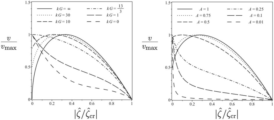
FIGURE 1. Bubble tip velocity as a function of curvature for various acceleration strengths when A = 1, and various Atwood numbers when kG = 30.

Figure 2 shows the shear function as a function of the bubble curvature for various values of A and kG, respectively. Figure 3 shows the bubble tip velocity as a function of the shear function for various values of A and kG, respectively.

FIGURE 2

FIGURE 2. Shear as a function of bubble curvature for various acceleration strengths when A = 1, and various Atwood numbers when kG = 30.

FIGURE 3

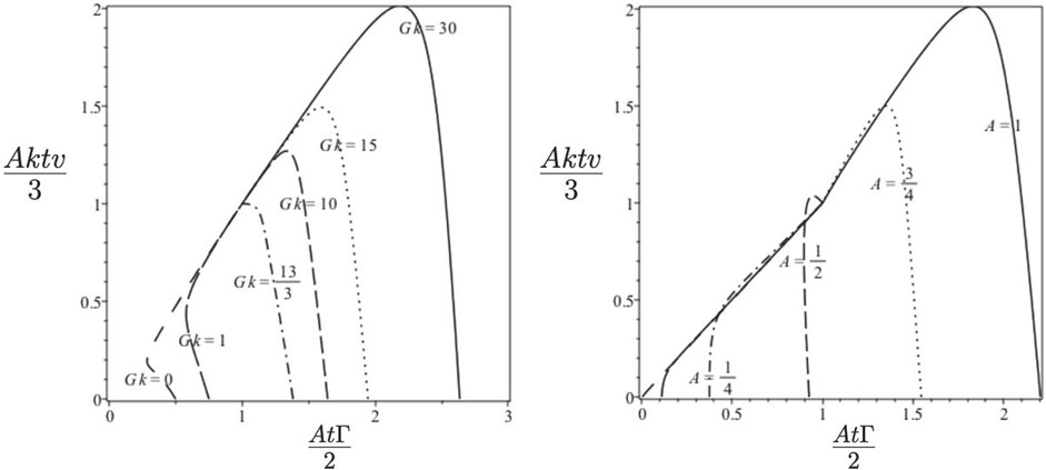
FIGURE 3. Bubble velocity as a function of shear for various acceleration strengths when A = 1, and various Atwood numbers when kG = 30.

For small curvature, $\widehat{\zeta }\approx 0$,

$v\left(t\right)\approx \frac{3}{Akt}-\frac{2\widehat{\zeta }\left(3A^{3}kG-5A^2-8\right)}{A^{2}kt},\mathrm{\Gamma }\left(t\right)\approx \frac{2}{At}-\frac{4\widehat{\zeta }\left(3A^{3}kG-5A^2-8\right)}{3A^{2}t}.(24)$

From the expansion Eq. 24, we observe that there exists a special value of the acceleration strength G_sep separating RM type bubbles from RT type bubbles:

$k{G}_{\text{sep}}=\frac{5A^2+8}{3A^3},(25)$

with kG_sep → 13/3 for A → 1, and kG_sep → 8/(3A³) → ∞ for A → 0. For G < G_sep the flat bubble is the fastest, similarly to classical RMI; it is also always true for the a <−2 case. For G > G_sep, the maximum growth-rate solution is a curved bubble, similarly to classical RTI; it is also always true for the a >−2 case [6, 8]. In all cases, the bubble tip velocity is larger for larger values of the Atwood number A.

As kG → ∞, the curvature of the fastest bubble approaches the curvature ${\widehat{\zeta }}_m$, which satisfies

${\widehat{\zeta }}_m^4-\frac{1}{A}{\widehat{\zeta }}_m^3+\frac{9}{32}{\widehat{\zeta }}_m^2-\frac{27}{4096}=0$

and by solving this for A and substituting into the Eq. 23 gives that the maximum velocity approaches v_m (t), where

$\frac{v_m\left(t\right)}{\sqrt{g/k}}={\left|8{\widehat{\zeta }}_m\right|}^{\frac{3}{2}}.$

This is a universal relation between the curvature and the maximum velocity (and in fact holds for any values of kG and A when g = Gt^a with a >−2). For kG finite, we find the relationship

$\frac{v_{\text{max}}\left(t\right)}{\sqrt{g/k}}=\frac{\left(9-{\widehat{\zeta }}_{\text{max}}^2\right)\left(-A{\widehat{\zeta }}_{\text{max}}^3+\frac{9}{16}{\widehat{\zeta }}_{\text{max}}^2-\frac{27}{1024}\right)}{12\left({\widehat{\zeta }}_{\text{max}}^4-\frac{1}{A}{\widehat{\zeta }}_{\text{max}}^3+\frac{9}{32}{\widehat{\zeta }}_{\text{max}}^2-\frac{27}{4096}\right)\sqrt{kG}},(26)$

where the curvature ${\widehat{\zeta }}_{\text{max}}$ of maximum velocity satisfies a nonic polynomial with coefficients which depend on A and kG. When A = 1, this reduces to the cubic equation

${\widehat{\zeta }}_{\text{max}}^3-\frac{3kG-11}{16}{\widehat{\zeta }}_{\text{max}}^2+\frac{31-9kG}{192}{\widehat{\zeta }}_{\text{max}}-\frac{3kG-13}{1024}=0$

and Eq. 26 reduces to

$\frac{v_{\text{max}}\left(t\right)}{\sqrt{g/k}}=\frac{\left(3+8{\widehat{\zeta }}_{\text{max}}\right)\left(3+16{\widehat{\zeta }}_{\text{max}}\right)}{9\left(1+8{\widehat{\zeta }}_{\text{max}}\right)}.$

When A = 1, the fastest bubble is a curved bubble when $kG>\frac{13}{3}$ and correspondingly, ${\widehat{\zeta }}_{\text{max}}<\frac{1}{8}$, as observed in Figure 1.

Asymptotic analysis of the case when kG is large leads to the result that the fastest bubble is that with approximate curvature

${\widehat{\zeta }}_{\text{max}}\approx {\widehat{\zeta }}_{\infty }+\frac{\left(9-64{\widehat{\zeta }}_{\infty }^2\right)\left(448{\widehat{\zeta }}_{\infty }^2-9\right)}{196608\sqrt{-2kG{\widehat{\zeta }}_{\infty }^7}}.(27)$

When A = 1, this is approximately

${\widehat{\zeta }}_{\text{max}}=-\frac{1}{8}+\frac{1}{12\sqrt{kG}}.$

The approximation Eq. 27 is accurate to within 2.2% for kG = 50, and to within 0.1% for kG = 1,000. The corresponding velocity is

$\frac{v_{\text{max}}\left(t\right)}{\sqrt{g/k}}\approx {\left(-8{\widehat{\zeta }}_{\infty }\right)}^{\frac{3}{2}}+\frac{8192{\widehat{\zeta }}_{\infty }^4+320{\widehat{\zeta }}_{\infty }^2-9}{32{\widehat{\zeta }}_{\infty }\sqrt{kG}}.(28)$

This approximation is accurate to within 0.7% for kG = 50, and to within 0.03% for kG = 1,000.

3.2.2 Spikes

The spike solutions are valid for curvatures $\widehat{\zeta }\in ({\widehat{\zeta }}_{\text{sing}},{\widehat{\zeta }}_{\text{cr}})$ where

$\frac{{\widehat{\zeta }}_{\text{sing}}}{{\widehat{\zeta }}_{\text{cr}}}=\frac{1-\sqrt{1-A^2}}{A}.$

Figure 4 shows the spike tip velocity as a function of the spike curvature for various values of A and kG, respectively. The velocity becomes singular at $\widehat{\zeta }={\widehat{\zeta }}_{\text{sing}}$, the value of which depends on the Atwood number. Figure 5 shows the spike shear function as a function of the spike curvature for various values of A and kG, respectively.

FIGURE 4

FIGURE 4. Spike tip velocity as a function of curvature for various acceleration strengths when A = 3/4, and various Atwood numbers when kG = 1.

FIGURE 5

FIGURE 5. Shear as a function of spike curvature for various acceleration strengths when A = 3/4, various Atwood numbers when kG = 1.

3.2.3 Special Solutions for Nonlinear Bubbles and Spikes

There are a number of solutions in the family of nonlinear solutions which deserve special attention. Here, we consider properties of these special solutions for bubbles and for spikes in details.

3.3 Special Solutions for nonlinear bubbles

To conveniently describe properties of special solutions for nonlinear bubbles, we introduce dimensionless variables

$\check{\mathrm{\zeta }}=-\frac{\mathrm{\zeta }}{k},\check{\upsilon }=\frac{Akt}{3}v\left(t\right),\check{\mathrm{\Gamma }}=\frac{At}{2}\mathrm{\Gamma }\left(t\right),$

and use superscript 0 to refer to the limit kG → 0 and superscript ∞ to refer to the limit kG → ∞.

3.3.1 The Critical Bubble

For the critical bubble the curvature, velocity and shear function are

${\check{\mathrm{\zeta }}}_{\text{cr}}=\frac{3}{8},{\check{\upsilon }}_{\text{cr}}=0,{\check{\mathrm{\Gamma }}}_{\text{cr}}=\frac{A}{4}\left[1+\sqrt{\frac{1+A\left(1+6kG\right)}{1+A}}\right],{\check{\mathrm{\Gamma }}}_{\text{cr}}^0=\frac{A}{2},{\check{\mathrm{\Gamma }}}_{\text{cr}}^{\infty }=\frac{\sqrt{6}}{4}\sqrt{\frac{kG{A}^3}{1+A}}.(29)$

This is a limiting-case solution, because bubbles in the family of solutions cannot be more curved than the critical bubble. For this bubble the velocity is zero and the shear alone maintains the pressure at the interface.

3.3.2 The Convergence-Limit Bubble

The magnitudes of the Fourier harmonics |Φ₁₀ (t)| and |Φ₂₀ (t)| coincide when $\check{\zeta }=5/24$. We define this to be the convergence-limit bubble solution. The curvature, velocity and shear function are

${\check{\zeta }}_{\text{cl}}=\frac{5}{24},{\check{\upsilon }}_{\text{cl}}=\frac{14A}{81}\left(\frac{81-25A+\sqrt{{\check{q}}_{\text{cl}}}}{45+53A}\right),{\check{\upsilon }}_{\text{cr}}^0=\frac{28}{81}\left(\frac{81-25A}{53A+45}\right),{\check{\upsilon }}_{\text{cr}}^{\infty }=\frac{14A}{27}\sqrt{\frac{30A}{53A+45}},$

${\check{\mathrm{\Gamma }}}_{\text{cl}}=\frac{81}{56}{\check{\upsilon }}_{\text{cl}},{\check{q}}_{\text{cl}}={\left(81-25A\right)}^2+270AkG\left(53A+45\right).(30)$

For any Atwood number, the convergence limit bubble is less curved than the critical bubble, ${\check{\zeta }}_{\text{cl}}/{\check{\zeta }}_{\text{cr}}=5/9$, and has larger velocity when compared to the critical bubble.

3.3.3 The Taylor Bubble

We call this bubble as a “Taylor bubble” because its curvature is the same as in the work [2] of Davis & Taylor except for a difference in the wave-vector value. The Taylor bubble curvature, velocity and shear function are

${\check{\zeta }}_{\mathrm{T}}=\frac{1}{8},{\check{\upsilon }}_{\mathrm{T}}=\frac{2A\left(3-A+\sqrt{{\check{q}}_{\mathrm{T}}}\right)}{3\left(5A+3\right)},{\check{\upsilon }}_{\mathrm{T}}^0=\frac{4A\left(3-A\right)}{3\left(5A+3\right)},{\check{\upsilon }}_{\mathrm{T}}^{\infty }=\frac{2A}{3}\sqrt{\frac{2A}{5A+3}},$

${\check{\mathrm{\Gamma }}}_{\mathrm{T}}=\frac{9}{8}{\check{\upsilon }}_{\mathrm{T}},{\check{q}}_{\mathrm{T}}={\left(3-A\right)}^2+2AkG\left(5A+3\right).(31)$

For any Atwood number, the Taylor bubble is less curved and has larger velocity and smaller shear when compared to the convergent limit bubble and the critical bubble.

3.3.4 The Minimum-Shear Bubble

For any Atwood number and acceleration strength, there is a solution which minimises the shear function. We call this the minimum-shear bubble. Its curvature is in general a cumbersome function on A and GK. For Gk → 0 and 0 < A < A* = 2/9, the curvature of this bubble is ζ_min/ζ_cr = 1. For Gk → ∞, the curvature of this bubble is ζ_min/ζ_cr = 0.

3.3.5 The Layzer-Drag Bubble

The family of bubbles has a solution with velocity $v/\sqrt{g/k}=\sqrt{2A/(1+A)}$ in the limit kG → ∞. We call the bubble with this curvature the Layzer-drag bubble since the drag model applies the above velocity rescaling in terms of the Atwood number to the single-mode Layzer first-order approximation at A = 1 [38, 55]. Experiments and simulations tend to compare well with this rescaling [32, 38, 55]. The dimensionless curvature of the Layzer-drag bubble depends only on the Atwood number A and satisfies the quintic equation

$4096\left(1+A\right){\check{\zeta }}^5-1152\left(1+A\right){\check{\zeta }}^3+64A{\check{\zeta }}^2+\left(33+81A\right)\check{\zeta }+9A=0.$

For fluids of very similar densities the curvature is ${\check{\zeta }}_{\text{LD}}(A=0)=(1/8)\sqrt{9-4\sqrt{3}}$, whereas for fluids with very different densities it is ${\check{\zeta }}_{\text{LD}}(A=1)=1/8$, suggesting that Layzer-drag bubble is more curved for A → 0 than for A → 1.

The curvature, the velocity and the shear function are complicated functions on the Atwood number A and the acceleration strength G

${\check{\zeta }}_{\text{LD}}={\check{\zeta }}_{\text{LD}}\left(A\right),{\check{\upsilon }}_{\text{LD}}={\check{\upsilon }}_{\text{LD}}\left({\check{\zeta }}_{\text{LD}},A,kG\right),{\check{\mathrm{\Gamma }}}_{\text{LD}}={\check{\mathrm{\Gamma }}}_{\text{LD}}\left({\check{\zeta }}_{\text{LD}},A,kG\right).(32)$

For G ≪ G_sep, for the Layzer-drag bubble $({\check{\zeta }}_{\text{LD}},{\check{\upsilon }}_{\text{LD}},{\check{\mathrm{\Gamma }}}_{\text{LD}})\to {({\check{\zeta }}_{\text{LD}},{\check{\upsilon }}_{\text{LD}},{\check{\mathrm{\Gamma }}}_{\text{LD}})}^0$; in agreement with the classical RMI [6], we obtain:

$A\to 0,{\check{\zeta }}_{\text{LD}}\to \frac{\sqrt{9-4\sqrt{3}}}{8},{\check{\upsilon }}_{\text{LD}}\to \frac{2A}{\sqrt{3\left(9-4\sqrt{3}\right)}},{\check{\mathrm{\Gamma }}}_{\text{LD}}\to \frac{3A}{2\sqrt{9-4\sqrt{3}}};$

$A\to 1,{\check{\zeta }}_{\text{LD}}\to \frac{1}{8},{\check{\upsilon }}_{\text{LD}}\to \frac{1}{3},{\check{\mathrm{\Gamma }}}_{\text{LD}}\to \frac{3}{8}.$

For G ≫ G_sep, for the Layzer-drag bubble $({\check{\zeta }}_{\text{LD}},{\check{\upsilon }}_{\text{LD}},{\check{\mathrm{\Gamma }}}_{\text{LD}})\to {({\check{\zeta }}_{\text{LD}},{\check{\upsilon }}_{\text{LD}},{\check{\mathrm{\Gamma }}}_{\text{LD}})}^{\infty }$; in agreement with the classical RTI [6], we obtain:

$A\to 0,{\check{\zeta }}_{\text{LD}}\to \frac{\sqrt{9-4\sqrt{3}}}{8},{\check{\upsilon }}_{\text{LD}}\to \frac{A}{3}\sqrt{2AGk},{\check{\mathrm{\Gamma }}}_{\text{LD}}\to \frac{A\sqrt{3}}{4}\sqrt{2AGk};$

$A\to 1,{\check{\zeta }}_{\text{LD}}\to \frac{1}{8},{\check{\upsilon }}_{\text{LD}}\to \frac{\sqrt{Gk}}{3},{\check{\mathrm{\Gamma }}}_{\text{LD}}\to \frac{3\sqrt{Gk}}{8}.$

Figure 6 consists of plots of the scaled velocity and scaled shear function as functions of the acceleration parameter kG for the Layzer-drag bubble.

FIGURE 6

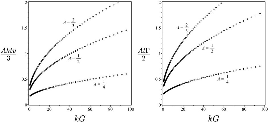
FIGURE 6. Layzer-drag (LD) bubble velocity and shear function as functions of acceleration parameter kG for various values of the Atwood number.

3.3.6 The Atwood Bubble

The fastest bubble of the family of solutions we refer to as the “Atwood bubble” in order to emphasise its dependence on the Atwood number. The Atwood bubble parameters are complicated functions of the Atwood number A and the acceleration strength G.

${\check{\zeta }}_{\mathrm{A}}={\check{\zeta }}_{\mathrm{A}}\left(A\right),{\check{\upsilon }}_{\mathrm{A}}={\check{\upsilon }}_{\mathrm{A}}\left({\check{\zeta }}_{\mathrm{A}},A,kG\right),{\check{\mathrm{\Gamma }}}_{\mathrm{A}}={\check{\mathrm{\Gamma }}}_{\mathrm{A}}\left({\check{\zeta }}_{\mathrm{A}},A,kG\right).(33)$

The acceleration G_sep, with kG_sep = (5A² + 8)/(3A³) in Eq. 25, separates the Atwood bubble solutions of RM type from those of RT type. If the acceleration strength is such that G < G_sep, then the maximum velocity Atwood bubble is the flat bubble and it is of RM type. If, however, G > G* then the fastest Atwood bubble is curved and is of RT type; its curvature depends on A and kG and is determined by maximising the velocity function Eq. 19.

For G < G_sep, the Atwood bubble is the flat bubble with the curvature, velocity and shear function

${\check{\zeta }}_{\mathrm{A}}=0,{\check{\upsilon }}_{\mathrm{A}}=1,{\check{\mathrm{\Gamma }}}_{\mathrm{A}}=1.$

For G > G_sep, the Atwood bubble is the curved bubble. Its velocity, curvature and shear functions depend on the Atwood number and the acceleration strength and are cumbersome. For G ≫ G_sep, for the Atwood bubble $({\check{\zeta }}_{\mathrm{A}},{\check{\upsilon }}_{\mathrm{A}},{\check{\mathrm{\Gamma }}}_{\mathrm{A}})\to {({\check{\zeta }}_{\mathrm{A}},{\check{\upsilon }}_{\mathrm{A}},{\check{\mathrm{\Gamma }}}_{\mathrm{A}})}^{\infty }$; in agreement with the classical RTI [6], we obtain:

$A\to 0,{\check{\zeta }}_{\mathrm{A}}\to \frac{3}{16}{A}^{\frac{1}{3}},{\check{\upsilon }}_{\mathrm{A}}\to \frac{A}{2}\sqrt{\frac{3}{2}AGk},{\check{\mathrm{\Gamma }}}_{\mathrm{A}}\to \frac{A}{2}\sqrt{\frac{3}{2}AGk};$

$A\to 1,{\check{\zeta }}_{\mathrm{A}}\to \frac{1}{8},{\check{\upsilon }}_{\mathrm{A}}\to \frac{\sqrt{Gk}}{3},{\check{\mathrm{\Gamma }}}_{\mathrm{A}}\to \frac{3\sqrt{Gk}}{8}.$

Figure 7 is a plot of the scaled curvature $\check{\zeta }=-\zeta /k$ as a function of the Atwood number A for the special critical, convergence limit, minimum shear, Taylor, Layzer-drag and Atwood bubbles. Figure 8 shows plots of their corresponding velocities and shear functions.

FIGURE 7

FIGURE 7. Scaled curvature as a function of the Atwood number for the critical (Cr), convergence-limit (CL), Taylor (T), minimum-shear (MS), Layzer-drag (LD) and Atwood (A) bubbles for kG = 30.

FIGURE 8

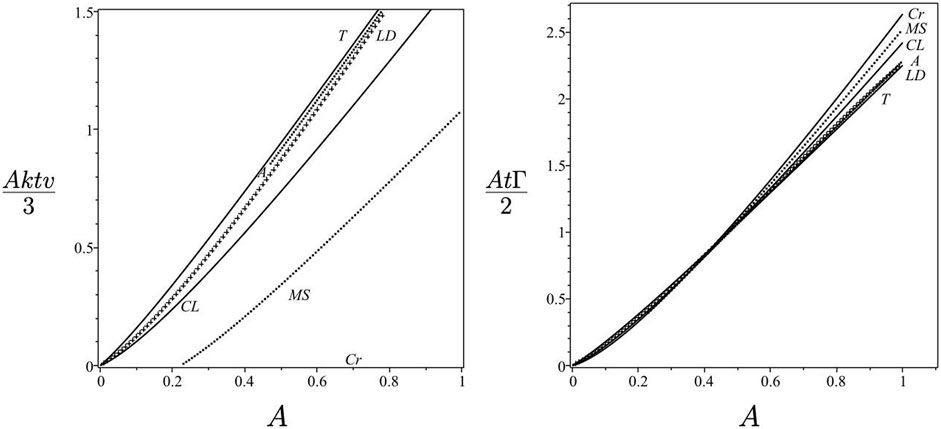
FIGURE 8. Velocity and shear function as functions of the Atwood number for the critical (Cr), convergence-limit (CL), Taylor (T), minimum-shear (MS), Layzer-drag (LD) and Atwood (A) bubbles bubbles for kG = 30.

3.4 Special Solutions for Nonlinear Spikes

To conveniently describe special solutions for nonlinear spikes, we introduce the dimensionless and negated variables

$\widehat{\zeta }=\frac{\zeta }{k},\widehat{v}=-\frac{Akt}{3}v\left(t\right),\widehat{\mathrm{\Gamma }}=-\frac{At}{2}\mathrm{\Gamma }\left(t\right)$

and use superscript 0 to refer to the limit kG → 0 and superscript ∞ to refer to the limit kG → ∞.

3.4.1 The Critical Spike

For the critical spike the curvature, velocity and shear function are

${\widehat{\zeta }}_{\text{cr}}=\frac{3}{8},{\widehat{v}}_{\text{cr}}=0,{\widehat{\mathrm{\Gamma }}}_{\text{cr}}=-\frac{A}{4}\left[1+\sqrt{\frac{1+\left(6kG-1\right)A}{1-A}}\right],{\widehat{\mathrm{\Gamma }}}_{\text{cr}}^0=-\frac{A}{2},{\widehat{\mathrm{\Gamma }}}_{\text{cr}}^{\infty }=\frac{\sqrt{6}}{4}\sqrt{\frac{kG{A}^3}{1-A}}.(34)$

3.4.2 The Convergence-Limit Spike

The magnitudes of the Fourier harmonics $|{\tilde{\mathrm{\Phi }}}_{10}(t)|$ and $|{\tilde{\mathrm{\Phi }}}_{20}(t)|$ coincide when $\widehat{\zeta }=5/24$. This defines the convergence-limit spike solution. The curvature, velocity, shear function and coefficients are

${\widehat{\zeta }}_{\text{cl}}=\frac{5}{24},{\widehat{v}}_{\text{cl}}=\frac{14A}{81}\left(\frac{25A+81+\sqrt{{\widehat{q}}_{\text{cl}}}}{53A-45}\right),{\widehat{v}}_{\text{cl}}^0=\frac{1}{3{\widehat{C}}_{\text{cl}}},{\widehat{v}}_{\text{cl}}^{\infty }=\frac{14A}{27}\sqrt{\frac{30A}{45-53A}},$

${\widehat{\mathrm{\Gamma }}}_{\text{cl}}=\frac{81}{56}{\widehat{v}}_{\text{cl}},{\widehat{q}}_{\text{cl}}={\left(25A+81\right)}^2+270AkG\left(45-53A\right).(35)$

3.4.3 The Taylor Spike

We refer to this spike as a ‘Taylor spike’ since its curvature is opposite to that of the Taylor bubble. The curvature, velocity, shear function and group-momentum coefficients are

${\widehat{\zeta }}_{\mathrm{T}}=\frac{1}{8},{\widehat{v}}_{\mathrm{T}}=\frac{2A\left(3+A+\sqrt{{\widehat{q}}_{\mathrm{T}}}\right)}{3\left(5A-3\right)}{\widehat{\mathrm{\Gamma }}}_{\mathrm{T}}=\frac{9}{8}{\widehat{v}}_{\mathrm{T}},{\widehat{q}}_{\mathrm{T}}={\left(3+A\right)}^2+2AkG\left(3-5A\right).(36)$

Note that ${\widehat{q}}_{\mathrm{T}}=0$ if $kG=\frac{{(3+A)}^2}{2A(5A-3)}$ and that for A > 3/5, the value of ${\widehat{q}}_{\mathrm{T}}$ will become negative for some finite positive value of kG. For example, if A = 3/4 then ${\widehat{q}}_{\mathrm{T}}<0$ if kG > 25/2.

3.4.4 The Layzer-drag spike

The family of spikes has a solution with velocity $v/\sqrt{g/k}=-\sqrt{2A/(1-A)}$ in the limit kG → ∞. We call the spike with this curvature the Layzer-drag spike solution since the drag model applies the above velocity rescaling using the Atwood number to the single-mode Layzer first-order approximation at A = 1 [38, 55]. Experimental results and numerical simulations tend to compare well with this re-scaling [32, 38, 55]. For the Layzer-drag spike, the dimensionless curvature depends on the Atwood number A and satisfies the quintic equation

$4096\left(1-A\right){\stackrel{̂;}{\zeta }}^5-1152\left(1-A\right){\widehat{\zeta }}^3+64A{\widehat{\zeta }}^2+\left(33-81A\right)\widehat{\zeta }+9A=0.$

For fluids of very similar densities, A ≈ 0, the curvature of the Layzer-drag spike is ${\check{\zeta }}_{\text{LD}}(A=0)=(\sqrt{9,-,4\sqrt{3}})/8$; it has the same magnitude as the Layzer-drag bubble. For fluids of very different densities, A ≈ 1, the curvature of the Layzer-drag spike is ${\widehat{\zeta }}_{\text{LD}}(A=1)=3/8$; its magnitude is three fold of that of the Layzer-drag bubble. For A ∈ (0, 1) the Layzer-drag spike is more curved than the Layzer-drag bubble.

The curvature, velocity and shear function of the Layzer-drag spike are complicated functions on the Atwood number A and acceleration strength G:

${\widehat{\zeta }}_{\text{LD}}={\widehat{\zeta }}_{\text{LD}}\left(A\right),{\widehat{v}}_{\text{LD}}={\widehat{v}}_{\text{LD}}\left({\widehat{\zeta }}_{\text{LD}},A,kG\right),{\widehat{\mathrm{\Gamma }}}_{\text{LD}}={\widehat{\mathrm{\Gamma }}}_{\text{LD}}\left({\widehat{\zeta }}_{\text{LD}},A,kG\right).(37)$

For Gk → 0, for the Layzer-drag spike $({\widehat{\zeta }}_{\text{LD}},{\widehat{v}}_{\text{LD}},{\widehat{\mathrm{\Gamma }}}_{\text{LD}})\to {({\widehat{\zeta }}_{\text{LD}},{\widehat{v}}_{\text{LD}},{\widehat{\mathrm{\Gamma }}}_{\text{LD}})}^0$; we obtain

$A\to 0,{\widehat{\zeta }}_{\text{LD}}\to \frac{\sqrt{9-4\sqrt{3}}}{8},{\widehat{\upsilon }}_{\text{LD}}\to \frac{2A}{\sqrt{3\left(9-4\sqrt{3}\right)}},{\widehat{\mathrm{\Gamma }}}_{\text{LD}}\to \frac{3A}{2\sqrt{9-4\sqrt{3}}};$

$A\to 1,{\widehat{\zeta }}_{\text{LD}}\to \frac{3}{8},{\widehat{\upsilon }}_{\text{LD}}\to \frac{11}{2}\sqrt{\frac{2}{1-A}},{\widehat{\mathrm{\Gamma }}}_{\text{LD}}\to \frac{11}{4\left(1-A\right)}.$

For Gk → ∞, for the Layzer-drag spike $({\widehat{\zeta }}_{\text{LD}},{\widehat{v}}_{\text{LD}},{\widehat{\mathrm{\Gamma }}}_{\text{LD}})\to {({\widehat{\zeta }}_{\text{LD}},{\widehat{v}}_{\text{LD}},{\widehat{\mathrm{\Gamma }}}_{\text{LD}})}^{\infty }$; in agreement with the classical RTI [6], we obtain

$A\to 0,{\widehat{\zeta }}_{\text{LD}}\to \frac{\sqrt{9-4\sqrt{3}}}{8},{\widehat{\upsilon }}_{\text{LD}}\to \frac{A}{3}\sqrt{2AGk},{\widehat{\mathrm{\Gamma }}}_{\text{LD}}\to \frac{A\sqrt{3}}{4}\sqrt{2AGk};$

$A\to 1,{\widehat{\zeta }}_{\text{LD}}\to \frac{3}{8},{\widehat{\upsilon }}_{\text{LD}}\to \frac{1}{3}\sqrt{\frac{2Gk}{1-A}},{\widehat{\mathrm{\Gamma }}}_{\text{LD}}\to \frac{\sqrt{Gk}}{6\left(1-A\right)}.$

Recall that spike solutions are only valid for curvatures $\widehat{\zeta }\in ({\widehat{\zeta }}_{\text{sing}},{\widehat{\zeta }}_{\text{cr}})$ where ${\widehat{\zeta }}_{\text{sing}}/{\widehat{\zeta }}_{\text{cr}}=(1-\sqrt{1-A^2})/A$.

Figure 9 consists of plots of the velocity and shear function of the Layzer-drag spike as functions of the acceleration parameter kG.

FIGURE 9

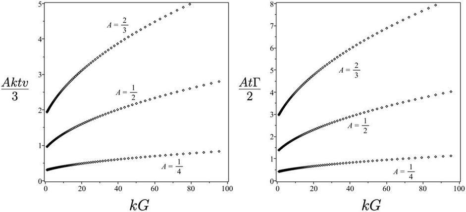
FIGURE 9. Layzer-drag (LD) spike scaled curvature and scaled shear function as functions of acceleration parameter kG for various values of the Atwood number.

Figure 10 is a plot of the scaled curvature $\widehat{\zeta }=\zeta /k$ as a function of the Atwood number A for the critical, convergence limit, Taylor and Layzer-drag spikes. Figure 11 illustrates the plots of their corresponding velocities and shear functions.

FIGURE 10

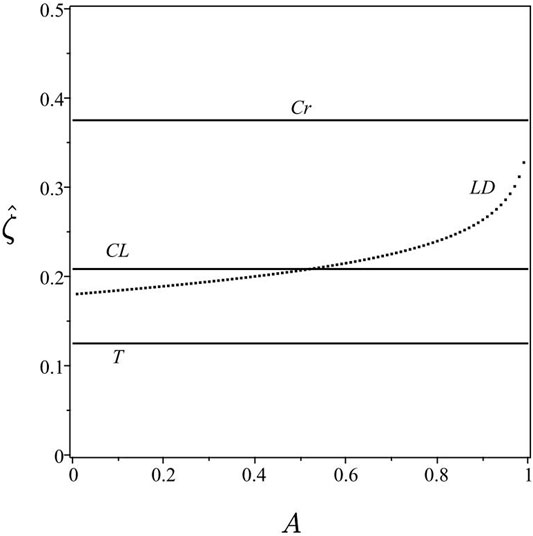
FIGURE 10. Scaled curvature as a function of the Atwood number for the critical (Cr), convergence-limit (CL), Taylor (T) and Layzer-drag (LD) spikes for kG = 30.

FIGURE 11

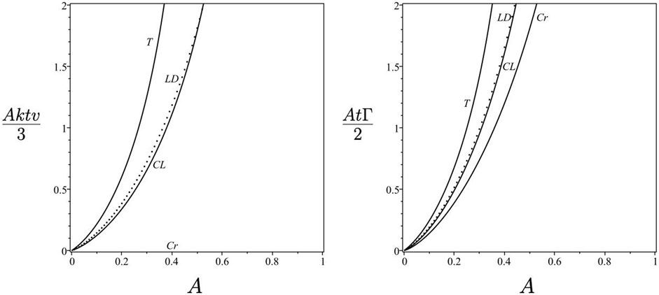
FIGURE 11. Velocity and shear function as functions of the Atwood number for the critical (Cr), convergence-limit (CL), Taylor (T) and Layzer-drag (LD) spikes for kG = 30.

3.4.5 The Atwood Spike

We refer to the fastest spike in the nonlinear family as the “Atwood spike”. The Atwood spike corresponds to the singular solution, and the solution is singular at any A and Gk. For the Atwood spike, the curvature has a finite value defined by the Atwood number A, whereas the velocity and the shear function are singular for any A and Gk:

${\widehat{\zeta }}_{\mathrm{A}}=\frac{3}{8}\frac{\left(1-\sqrt{1-A^2}\right)}{A},{\widehat{v}}_{\mathrm{A}}={\widehat{v}}_{\mathrm{A}}\left({\widehat{\zeta }}_{\mathrm{A}},A,kG\right)\to \infty ,{\widehat{\mathrm{\Gamma }}}_{\mathrm{A}}={\widehat{\mathrm{\Gamma }}}_{\mathrm{A}}\left({\widehat{\zeta }}_{\mathrm{A}},A,kG\right)\to \infty .(38)$

For Gk → 0, for the Atwood spike $({\widehat{\zeta }}_{\mathrm{A}},{\widehat{v}}_{\mathrm{A}},{\widehat{\mathrm{\Gamma }}}_{\mathrm{A}})\to {({\widehat{\zeta }}_{\mathrm{A}},{\widehat{v}}_{\mathrm{A}},{\widehat{\mathrm{\Gamma }}}_{\mathrm{A}})}^0$; we obtain:

$A\to 0,{\widehat{\zeta }}_{\mathrm{A}}\to \frac{3}{16}A,{\widehat{v}}_{\mathrm{A}}\to \frac{4}{A^2},{\widehat{\mathrm{\Gamma }}}_{\mathrm{A}}\to \frac{4}{A^2};$

$A\to 1,{\widehat{\zeta }}_{\mathrm{A}}\to \frac{3}{8},{\widehat{v}}_{\mathrm{A}}\to \frac{11}{2}\sqrt{\frac{2}{1-A}},{\widehat{\mathrm{\Gamma }}}_{\mathrm{A}}\to \frac{11}{4\left(1-A\right)}.$

For Gk → ∞, for the Atwood spike $({\widehat{\zeta }}_{\mathrm{A}},{\widehat{v}}_{\mathrm{A}},{\widehat{\mathrm{\Gamma }}}_{\mathrm{A}})\to {({\widehat{\zeta }}_{\mathrm{A}},{\widehat{v}}_{\mathrm{A}},{\widehat{\mathrm{\Gamma }}}_{\mathrm{A}})}^{\infty }$, and we obtain:

$A\to 0,{\widehat{\zeta }}_{\mathrm{A}}\to \frac{3}{16}A,{\widehat{v}}_{\mathrm{A}}\to \sqrt{\frac{3Gk}{A}},{\widehat{\mathrm{\Gamma }}}_{\mathrm{A}}\to \sqrt{\frac{3Gk}{A}};$

$A\to 1,{\widehat{\zeta }}_{\mathrm{A}}\to \frac{3}{8},{\widehat{v}}_{\mathrm{A}}\to \sqrt{\frac{2Gk}{1-A}},{\widehat{\mathrm{\Gamma }}}_{\mathrm{A}}\to \frac{\sqrt{Gk}}{2\left(1-A\right)}.$

We emphasize that, independently of the acceleration strength G, the curvature of the Atwood spike $({\widehat{\zeta }}_{\mathrm{A}}/{\widehat{\zeta }}_{\text{cr}})\to 1$ for A → 1 and $({\widehat{\zeta }}_{\mathrm{A}}/{\widehat{\zeta }}_{\text{cr}})\to 0$ for A → 0. This suggests that the fastest Atwood spike has the same curvature magnitude in RT and RM cases. For fluids of very similar densities, A → 0 the Atwood spike curvature is $\widehat{\zeta }\to (3/16)A$, whereas for fluids of very different densities, A → 1, it is $\widehat{\zeta }\to 3/8$. The singular values of the velocity and the shear function of the Atwood spike indicate that the nonlinear spikes can move faster and have the shear increasing with time quicker than ∼ t⁻¹; for instance, the velocity and shear function of the spike can change with time as $\sim t^{\gamma }$ with γ >−1.

3.5 Qualitative Properties of RT/RM Dynamics

3.5.1 Interfaciality

Our analysis accurately accounts for the interplay of harmonics and systematically connects the interfacial velocity and shear. We find that for RTI and RMI driven by the inverse-quadratic power-law acceleration, the dynamics is essentially interfacial, has intense fluid motion in the vicinity of the interface and has effectively no motion away from it. Shear-driven vortical structures may appear at the interface due to the interfacial shear. The velocity field in the bulk of each fluid is potential.

3.5.2 Multiscale Character

Our analysis suggests that for both bubbles and spikes, nonlinear RT/RM dynamics is multiscale, having two contributing macroscopic length scales, these being the wavelength and the amplitude. This multi-scale character can be understood by interpreting the coherent structure as a standing wave of growing amplitude.

3.5.3 RT-to-RM Transition

Our analysis finds that for small values of the acceleration strength, kG ≪ 1, the dynamics is qualitatively similar to that of classical Richtmyer-Meshkov instability, whereas for large values of the acceleration strength, kG ≫ 1, the dynamics is similar to that of classical Rayleigh-Taylor instability.

In the linear regime, RT-to-RM transition occurs with the decrease of the acceleration strength kG for the bubble and for the spike. In the nonlinear regime, the fastest RM bubble is the flat bubble, whereas the fastest RT bubble is a curved bubble with the curvature value dependent on the Atwood number. For nonlinear bubbles, a transition from RM dynamics to RT dynamics happens as the dimensionless parameter kG passes through the separation value kG_sep = (5A² + 8)/2A³. Our analysis hence provides for nonlinear bubbles the quantitative dependence of the acceleration strength on the density ratio, at which RT-to-RM transition occurs (for the first time, to the best of the authors’ knowledge).

For nonlinear spikes the fastest spike has the same curvature magnitude in RM and RT cases; it depends on the Atwood number and is independent of the acceleration strength kG. The velocity and the shear function of the fastest spike are singular, suggesting that for any value of the acceleration strength kG the RT/RM spike can move faster than the nonlinear asymptotic solutions prescribe; for instance, its velocity and shear function can change with time as $\sim t^{\gamma }$ with γ > −1.

3.6 Comparison With Observations

In classical RTI/RMI, RT bubbles and spikes move significantly faster than RM bubbles and spikes in either linear or nonlinear regime. Hence, experiments and simulations can differentiate between RT dynamics and RM dynamics by measuring the growth-rate of RT/RM bubbles/spikes [18, 20, 21, 27, 32, 33, 45, 52–54]. For variable acceleration g = G/t² considered in the present work, RT/RM bubbles and spikes move slowly in the linear regime, and have nonlinear asymptotic solutions changing with time as $\sim 1/t$ in the nonlinear regime. To accurately identify a pre-factor of a power-law, a substantially span of temporal and spatial scales is required, which is usually very challenging to achieve in experiments and simulations [45, 56]. An accurate implementation of the acceleration with the magnitude g = G/t² is also challenging. Nevertheless, since our analysis finds that, expect for the time-dependence, the properties of RT/RM dynamics of bubbles/spikes are similar in many regards to those of classical RTI/RMI, we may compare our analysis with existing experiments and simulations. Our theoretical results are in agreement with available observations [18, 20, 21, 27, 32, 33, 45, 52–54].

Particularly, our theory accurately reproduces the interfaciality of RT/RM dynamics, which is observed in experiments and simulations. This includes the velocity field with intense motion of the fluids in a vicinity of the interface, with effectively no motion away from the interface, and with vortical structures produced by shear at the interface [20–22, 27, 45]. Our analysis further finds that in the nonlinear regime RT bubbles are curved and RM bubbles are flat. The flattening of RM bubble front and the curved shape of RT bubble are distinct feature of nonlinear RMI and RTI, respectively; they are observed in experiments and simulations in fluids and plasmas [18, 20, 21, 27, 32, 33, 45, 52–54]. Our analysis also finds that, at any density ratio and acceleration strength, nonlinear RT/RM spikes can achieve a finite curvature magnitude and can move with a time-dependence faster than that of nonlinear RT/RM bubbles, in agreement with observations [18, 20, 21, 27, 32, 33, 45, 52–54].

In RTI, experiments and simulations tend to compare well with the velocity of nonlinear Layzer-drag bubble $\sqrt{g/k}\sqrt{2A/(1+A)}$ and the velocity of nonlinear Layzer-drag spike $\sqrt{g/k}\sqrt{2A/(1-A)}$ [32]. Our group theory approach provides the (only one, to the best of the authors’ knowledge) rigorous derivation of the Layzer-drag solutions for bubbles and spikes in RTI with variable acceleration, which have physically justifiable velocity fields and which are fully consistent with the complete set of the governing equations, Eqs 1–3). Furthermore, we find that curvatures of the Layzer-drag bubble and spike depend on the density ratio. The Layzer-drag spike is more curved than the bubble for fluids with very different densities, A → 1, and has the same curvature magnitude for fluids with very similar densities, A → 0. These results can be applied for verification and validation of numerical models and for comparison with experiments [7, 18, 32].

The group theory approach also provides the (first, to the best of the authors’ knowledge) rigorous derivation of the Layzer-drag solutions for bubbles and spikes in RMI with variable acceleration [32, 33, 53]. Particularly, in RMI, we define the Layzer-drag bubble and spike as solutions which have, for a given Atwood number A, the same respective curvature values as the Layzer-drag bubble and spike in RTI. We further transition in RT/RM family of nonlinear solutions with variable acceleration, g = Gt^a and a = − 2, from the RT limit, kG → ∞, to the RM limit, kG → 0.

Our group theory approach explains why in RTI simulations, for nonlinear bubble the velocity magnitude can be somewhat slower and the curvature magnitude can be somewhat larger compared to those corresponding to the fastest theoretical solutions. These departures can be understood by recalling that the theory studies the dynamics of ideal fluids and finds a family of nonlinear solutions parameterized by the interfacial shear, whereas numerical simulations usually model viscous fluids with a shear-free velocity at the interface. Due to the presence of finite viscosity in the simulations, a larger shear and a more curved surface of RT bubble is required to maintain the pressure at the interface, in agreement with our theory. For nonlinear RMI, the fastest bubble with the largest shear is the flat bubble, and the flattening of the bubble front is observed in RMI simulations, in agreement with our theory [18, 20, 21, 27, 32, 33, 45, 52–54].

RT/RM experiments and simulations are usually focused on the diagnostics of the growth of the amplitude in the linear and nonlinear regimes [18, 20, 21, 27, 32, 45, 52–54]. We identify the growth and the growth-rate of the amplitude, and we also the elaborate the properties of the linear and nonlinear RT/RM solutions, which were not diagnosed before and which can be applied for design of future experiments and simulations. These include: the dependence of the velocity and the morphology of RT/RM bubbles/spikes on the density ratio and the acceleration strength; the properties of RT-to-RM transition for linear/nonlinear bubbles/spikes; the dependence of the interfacial shear and the interfacial vortical structures on the acceleration parameters and density ratio; the qualitative and quantitative properties of the velocity and pressure fields. According to our theoretical results, in realistic environments and for variable acceleration g = Gt^a with a = −2, for an accurate quantification of the linear and nonlinear stages of RTI/RMI, new approaches are required to achieve the high accuracy, high precision and the large span of spatial and temporal scales in the observational data in experiments and simulations [56].

4 Discussion

We have studied RT/RM instabilities induced by an acceleration having an inverse-quadratic power-law time dependence, and considered a broad range of acceleration strengths and density ratios, for a three-dimensional spatially extended period flow with square symmetry in the plane normal to the acceleration. By applying the group theory approach, we have found solutions for the early-time linear and late-time nonlinear dynamics of RT/RM coherent structures of bubbles and spikes, and have thoroughly investigated the dependence of the solutions on the acceleration parameters and initial conditions. Our analysis reveals that the dynamics is of RT type for strong accelerations and is of RM type for weak accelerations, and investigates the dependence of RT-to-RM transition on the acceleration magnitude and fluid density ratio. To our knowledge, this detailed analysis has never been performed before.

In the early-time regime, RT/RM dynamics is single-scale and is set by the structure’s spatial period. The dynamics is well captured by the lowest-order harmonics, the solution is being unique for given spatial period, acceleration, fluid density ratio, and initial conditions. The formation of RT/RM bubbles/spike is determined by the initial conditions, with the bubble (spike) moving up (down) and being concave down (up). In the late-time regime RT/RM dynamics of bubbles/spikes is multi-scale and is set by the structure’s spatial period and amplitude. The nonlinear dynamics requires one to account for multiple harmonics. For given values of the spatial period, acceleration strength, fluid density ratio and initial growth-rate, there is a continuous family of nonlinear solutions for RT/RM bubbles/spikes. This non-uniqueness is due to the interfacial shear. The family of solutions can be parameterised by the interface morphology (i.e., the principal curvature at the bubble/spike tip) and/or by the interfacial shear. The dynamics of RT/RM bubbles/spikes is essentially interfacial, with intense fluid motion near the interface and effectively no fluid motion away from it. The velocity field is potential in the bulk, and vortical structures are produced by shear at the interface. These results are in excellent qualitative agreement with available observations [20, 23–33].

In the early-time regime, RT/RM bubbles and spikes evolve “symmetrically”. In the late-time regime, bubbles are regular whereas spikes can be singular and move faster than the nonlinear asymptotic solutions prescribes. A number of special solutions are identified in the family of nonlinear solutions for RT/RM bubbles/spikes, including critical solutions with largest curvature values, the convergence limit solutions, the Taylor solutions with constant curvature magnitudes, the minimum shear solutions, the Layzer-drag solutions and the fastest Atwood solutions. We define the Layzer-drag solutions by using the velocity re-scaling of RT bubbles/spikes with which observations tend to compare well, and we elaborate the dependence of the curvature and the velocity magnitudes on the fluid density ratio over a broad range of acceleration magnitudes, including the RT type limit of large accelerations and the RM type limit of small accelerations. For RT/RM bubbles, the fastest Atwood solution corresponds to the curved bubble in the RT limit of strong accelerations and to the flat bubble in the RM limit of weak accelerations. For RT/RM spikes, the fastest Atwood solution corresponds to the curved spike with singular velocity and shear and with the same curvature value in the RT and RM limits. These results can be compared with future observations [6–8, 18, 20, 23–33].

Our analysis captures the physics of linear and nonlinear RT/RM dynamics induced by variable acceleration and also RT-to-RM transition. Our theory can be extended to higher orders, including spatial expansion of the governing equations and the Fourier harmonics of the heavy and light fluids, leading to minor quantitative corrections, similarly to previous work [40, 41]. Our analysis can also be extended to other symmetries and dimensionalities, including two-dimensional flows and three-dimensional flows with, e.g., hexagonal, rhombic and rectangular symmetries in the plane normal to the acceleration direction [6, 8]. This permits the systematic investigation of linear and nonlinear RT/RM dynamics and RT-to-RM transition as well as properties of the dimensional 3D-to-2D crossover, to be done in the future.

Our present work is focused on RT/RM dynamics driven by variable accelerationa g = Gt^a with a = −2 and RT-to-RM transition for ideal incompressible fluids. While this approximation is reasonable and is held even for strong-shock-driven RMI [20, 22, 27], a systematic theoretical study is required of RT/RM dynamics and RT-to-RM transition for compressible and viscous fluids. The study is especially important for purposes of comparison of the theory with the simulations. We address to the future the systematic investigations of the effect of compressibility and viscosity on RT/RM dynamics.

Our analysis has investigated the dependence of RT-to-RM transition on the fluid density ratio and on the acceleration strength for both linear and nonlinear dynamics, it agrees qualitatively with available observations [20, 23–33], and elaborates extensive theory benchmarks, not diagnosed before, for future experiments and simulations. These include, for instance, the velocity and pressure fields, the interface morphology and bubble/spike curvatures, the interfacial shear and its link to the bubble/spike velocities and curvatures, the spectral properties of the velocity and pressure, along with the interface growth and growth rate. By identifying these properties and comparing them to data obtained for actual fluids, we may further enhance our knowledge of RT/RM dynamics in realistic environments [8–18]. And hence achieve a better understanding of RT/RM relevant processes in Nature and technology [8–18]. We can also help to improve numerical modeling and experimental diagnostics of the interfacial dynamics of fluids, plasmas and materials [20, 23–33].

Data Availability Statement

The original contributions presented in the study are included in the article/Supplementary Material, further inquiries can be directed to the corresponding author.

Author Contributions

DH: Investigation, formal analysis, writing—original draft. SA: Conceptualisation, investigation formal analysis, methodology, project administration, writing - original draft and revision.

Conflict of Interest

The authors declare that the research was conducted in the absence of any commercial or financial relationships that could be construed as a potential conflict of interest.

Publisher’s Note

All claims expressed in this article are solely those of the authors and do not necessarily represent those of their affiliated organizations, or those of the publisher, the editors and the reviewers. Any product that may be evaluated in this article, or claim that may be made by its manufacturer, is not guaranteed or endorsed by the publisher.

Acknowledgments

The authors thank the University of Western Australia (AUS) and the National Science Foundation (United States).

References

1. Rayleigh, L. Investigations of the Character of the Equilibrium of an Incompressible Heavy Fluid of Variable Density. Proc Lond Math Soc (1883) 14:170–7.

Google Scholar

2. Davies, R, and Taylor, G. The Mechanics of Large Bubbles Rising through Extended Liquids and through Liquids in Tubes. Proc R Soc A (1950) 200:375–90.

Google Scholar

3. Richtmyer, RD. Taylor Instability in Shock Acceleration of Compressible Fluids. Comm Pure Appl Math (1960) 13:297–319. doi:10.1002/cpa.3160130207

CrossRef Full Text | Google Scholar

4. Meshkov, E. Instability of the Interface of Two Gases Accelerated by a Shock. Sov Fluid Dyn (1969) 4:101–4.

Google Scholar

5. Abarzhi, S, and Sreenivasan, K. Turbulent Mixing and beyond. London, UK: The Royal Society (2010). ISBN 085403806X.

Google Scholar

6. Abarzhi, SI. Review of Theoretical Modelling Approaches of Rayleigh-Taylor Instabilities and Turbulent Mixing. Phil Trans R Soc A (2010) 368:1809–28. doi:10.1098/rsta.2010.0020

PubMed Abstract | CrossRef Full Text | Google Scholar

7. Anisimov, SI, Drake, RP, Gauthier, S, and Meshkov, SI. What Is Certain and what Is Not So Certain in Our Knowledge of Rayleigh-taylor Mixing? Phil Trans R Soc A (2013) 371:20130266. doi:10.1098/rsta.2013.0266

PubMed Abstract | CrossRef Full Text | Google Scholar

8. Abarzhi, SI, Bhowmick, A, Naveh, A, Pandian, A, Swisher, N, Stellingwerf, R, et al. Supernova, Nuclear Synthesis, Fluid Instabilities and Interfacial Mixing. Proc Natl Acad Sci USA (2018) 201714502. doi:10.1073/pnas.1714502115

CrossRef Full Text | Google Scholar

9. Arnett, D. Supernovae and Nucleosynthesis: An Investigation of the History of Matter, from the Big Bang to the Present. Princeton University Press (1996).

Google Scholar

10. Mahalov, A. Multiscale Modeling and Nested Simulations of Three-Dimensional Ionospheric Plasmas: Rayleigh-Taylor Turbulence and Nonequilibrium Layer Dynamics at fine Scales. Phys Scr (2014) 89:098001. doi:10.1088/0031-8949/89/9/098001

CrossRef Full Text | Google Scholar

11. Rana, S, and Herrmann, M. Primary Atomization of a Liquid Jet in Crossflow. Phys Fluids (2011) 23:091109. doi:10.1063/1.3640022

CrossRef Full Text | Google Scholar

12. Buehler, MJ, Tang, H, van Duin, ACT, and Goddard, WA. Threshold Crack Speed Controls Dynamical Fracture of Silicon Single Crystals. Phys Rev Lett (2007) 99:165502. doi:10.1103/physrevlett.99.165502

PubMed Abstract | CrossRef Full Text | Google Scholar

13. Peters, N. Turbulent Combustion. Cambridge University Press (2000).

Google Scholar

14. Drake, RP. Perspectives on High-Energy-Density Physics. Phys Plasmas (2009) 16:055501. doi:10.1063/1.3078101

CrossRef Full Text | Google Scholar

15. Zeldovich, Y, and Raizer, Y. Physics of Shock Waves and High-Temperature Hydrodynamic Phenomena. New York: Dover (2002).

Google Scholar

16. Sedov, L. Similarity and Dimensional Methods in Mechanics. Boca Raton, FL: CRC Press (1993).

Google Scholar

17. Landau, L, and Lifshitz, E. Course of Theoretical Physics. New York: Pergamon Press (1987).

Google Scholar

18. Meshkov, EE, and Abarzhi, SI. Group Theory and Jelly's experiment of Rayleigh-Taylor Instability and Rayleigh-Taylor Interfacial Mixing. Fluid Dyn Res (2019) 51:065502. doi:10.1088/1873-7005/ab3e83

CrossRef Full Text | Google Scholar

19. I Abarzhi, S. Review of Nonlinear Dynamics of the Unstable Fluid Interface: Conservation Laws and Group Theory. Phys Scr (2008) T132:014012. doi:10.1088/0031-8949/2008/t132/014012

CrossRef Full Text | Google Scholar

20. Stanic, M, Stellingwerf, RF, Cassibry, JT, and Abarzhi, SI. Scale Coupling in Richtmyer-Meshkov Flows Induced by strong Shocks. Phys Plasmas (2012) 19:082706. doi:10.1063/1.4744986

CrossRef Full Text | Google Scholar

21. Dell, Z, Stellingwerf, RF, and Abarzhi, SI. Effect of Initial Perturbation Amplitude on Richtmyer-Meshkov Flows Induced by strong Shocks. Phys Plasmas (2015) 22:092711. doi:10.1063/1.4931051

CrossRef Full Text | Google Scholar

22. Dell, ZR, Pandian, A, Bhowmick, AK, Swisher, NC, Stanic, M, Stellingwerf, RF, et al. Maximum Initial Growth-Rate of strong-shock-driven Richtmyer-Meshkov Instability. Phys Plasmas (2017) 24:090702. doi:10.1063/1.4986903

CrossRef Full Text | Google Scholar

23. Remington, B. Rayleigh-taylor Instabilities in High-Energy Density Settings on the National Ignition Facility. Proc Natl Acad Sci USA (2018) 201717236. doi:10.1073/pnas.1717236115

CrossRef Full Text | Google Scholar

24. Lugomer, S. Laser-generated Richtmyer–Meshkov and Rayleigh–taylor Instabilities. Iii. Nearperipheral Region of Gaussian Spot. Laser Part Beams (2016) 35:597–609.

Google Scholar

25. Akula, B, Suchandra, P, Mikhaeil, M, and Ranjan, D. Dynamics of Unstably Stratified Free Shear Flows: an Experimental Investigation of Coupled Kelvin-Helmholtz and Rayleigh-taylor Instability. J Fluid Mech (2017) 816:619–60. doi:10.1017/jfm.2017.95

CrossRef Full Text | Google Scholar

26. Read, K. Experimental Investigation of Turbulent Mixing by Rayleigh–taylor Instability. Physica D (1984) 12:398–400. doi:10.1016/0167-2789(84)90513-x

CrossRef Full Text | Google Scholar

27. Meshkov, E. Some peculiar Features of Hydrodynamic Instability Development. Phil Trans R Soc A (2013) 371:20120288. doi:10.1098/rsta.2012.0288

PubMed Abstract | CrossRef Full Text | Google Scholar

28. Kucherenko, Y. Experimental Study into the Rayleigh-taylor Turbulent Mixing Zone Heterogeneous Structure. Laser Part Beams (1975) 21:375.

Google Scholar

29. Glimm, J, Sharp, DH, Kaman, T, and Lim, H. New Directions for Rayleigh-taylor Mixing. Phil Trans R Soc A (2013) 371:20120183. doi:10.1098/rsta.2012.0183

PubMed Abstract | CrossRef Full Text | Google Scholar

30. Kadau, K, Barber, JL, Germann, TC, Holian, BL, and Alder, BJ. Atomistic Methods in Fluid Simulation. Phil Trans R Soc A (2010) 368:1547–60. doi:10.1098/rsta.2009.0218

PubMed Abstract | CrossRef Full Text | Google Scholar

31. Youngs, DL. The Density Ratio Dependence of Self-Similar Rayleigh-taylor Mixing. Phil Trans R Soc A (2013) 371:20120173. doi:10.1098/rsta.2012.0173

PubMed Abstract | CrossRef Full Text | Google Scholar

32. Dimonte, G, Youngs, DL, Dimits, A, Weber, S, Marinak, M, Wunsch, S, et al. A Comparative Study of the Turbulent Rayleigh-taylor Instability Using High-Resolution Three-Dimensional Numerical Simulations: The Alpha-Group Collaboration. Phys Fluids (2004) 16:1668–93. doi:10.1063/1.1688328

CrossRef Full Text | Google Scholar

33. Thornber, B, Griffond, J, Poujade, O, Attal, N, Varshochi, H, Bigdelou, P, et al. Late-time Growth Rate, Mixing, and Anisotropy in the Multimode Narrowband Richtmyer-Meshkov Instability: The θ-group Collaboration. Phys Fluids (2017) 29:105107. doi:10.1063/1.4993464

CrossRef Full Text | Google Scholar

34. Chandrasekhar, S. Hydrodynamic and Hydromagnetic Stability. Oxford University Press (1961).

Google Scholar

35. Kull, HJ. Theory of the Rayleigh-taylor Instability. Phys Rep (1991) 206:197–325. doi:10.1016/0370-1573(91)90153-d

CrossRef Full Text | Google Scholar

36. Nishihara, K, Wouchuk, JG, Matsuoka, C, Ishizaki, R, and Zhakhovsky, VV. Richtmyer-meshkov Instability: Theory of Linear and Nonlinear Evolution. Phil Trans R Soc A (2010) 368:1769–807. doi:10.1098/rsta.2009.0252

PubMed Abstract | CrossRef Full Text | Google Scholar

37. Berning, M, and Rubenchik, AM. A Weakly Nonlinear Theory for the Dynamical Rayleigh-Taylor Instability. Phys Fluids (1998) 10:1564–87. doi:10.1063/1.869677

CrossRef Full Text | Google Scholar

38. Layzer, D. On the Instability of Superposed Fluids in a Gravitational Field. ApJ (1955) 122:1. doi:10.1086/146048

CrossRef Full Text | Google Scholar

39. Garabedian, P. On Steady-State Bubbles Generated by taylor Instability. Proc R Soc A (1957) 241:423.

Google Scholar

40. Abarzhi, SI. Stable Steady Flows in Rayleigh-Taylor Instability. Phys Rev Lett (1998) 81:337–40. doi:10.1103/physrevlett.81.337

CrossRef Full Text | Google Scholar

41. Abarzhi, SI, Nishihara, K, and Rosner, R. Multiscale Character of the Nonlinear Coherent Dynamics in the Rayleigh-taylor Instability. Phys Rev E Stat Nonlin Soft Matter Phys (2006) 73:036310. doi:10.1103/PhysRevE.73.036310

PubMed Abstract | CrossRef Full Text | Google Scholar

42. Abarzhi, SI. The Stationary Spatially Periodic Flows in Rayleigh-Taylor Instability: Solutions Multitude and its Dimension. Phys Scr (1996) T66:238–42. doi:10.1088/0031-8949/1996/t66/044

CrossRef Full Text | Google Scholar

43. Abarzhi, SI. Stable Steady Flows in Rayleigh-taylor Instability. Phys Rev Lett (1998) 81:337–40. doi:10.1103/physrevlett.81.337

CrossRef Full Text | Google Scholar

44. Abarzhi, SI. A New Type of the Evolution of the Bubble Front in the Richtmyer-Meshkov Instability. Phys Lett A (2002) 294:95–100. doi:10.1016/s0375-9601(02)00036-1

CrossRef Full Text | Google Scholar

45. Herrmann, M, Moin, P, and Abarzhi, SI. Nonlinear Evolution of the Richtmyer-Meshkov Instability. J Fluid Mech (2008) 612:311–38. doi:10.1017/s0022112008002905

CrossRef Full Text | Google Scholar

46. Hill, DL, and Abarzhi, SI. On the Rayleigh-Taylor Unstable Dynamics of Three-Dimensional Interfacial Coherent Structures with Time-dependent Acceleration. AIP Adv (2019) 9:075012. doi:10.1063/1.5116870

CrossRef Full Text | Google Scholar

47. Abarzhi, SI, and Williams, KC. Scale-dependent Rayleigh-taylor Dynamics with Variable Acceleration by Group Theory Approach. Phys Plasmas (2020) 27:072107. doi:10.1063/5.0012035

CrossRef Full Text | Google Scholar

48. Hill, DL, and Abarzhi, SI. Richtmyer-meshkov Dynamics with Variable Acceleration by Group Theory Approach. Appl Math Lett (2020) 105:106338. doi:10.1016/j.aml.2020.106338

CrossRef Full Text | Google Scholar

49. Hill, DL, Bhowmich, AK, Ilyin, DV, and Abarzhi, SI. Group Theory Analysis of Early-Time Scale-dependent Dynamics of the Rayleigh-taylor Instability with Time Varying Acceleration. Phys Rev Fluids (2019) 4:063905. doi:10.1103/physrevfluids.4.063905

CrossRef Full Text | Google Scholar

50. Williams, KC, and Abarzhi, SI. Effect of Dimensionality and Symmetry on Scale-dependent Dynamics of Rayleigh-taylor Instability. Fluid Dyn Res (2021) 53:035507. doi:10.1088/1873-7005/ac06d7

CrossRef Full Text | Google Scholar

51. Schlichting, H, and Gersten, K. Boundary-Layer Theory. Springer (2004).

Google Scholar

52. Motl, B, Oakley, J, Ranjan, D, Weber, C, Anderson, M, and Bonazza, R. Experimental Validation of a Richtmyer-Meshkov Scaling Law over Large Density Ratio and Shock Strength Ranges. Phys Fluids (2009) 21:126102. doi:10.1063/1.3280364

CrossRef Full Text | Google Scholar

53. Jacobs, JW, and Krivets, VV. Experiments on the Late-Time Development of Single-Mode Richtmyer-Meshkov Instability. Phys Fluids (2005) 17:034105. doi:10.1063/1.1852574

CrossRef Full Text | Google Scholar

54. Glendinning, SG, Bolstad, J, Braun, DG, Edwards, MJ, Hsing, WW, Lasinski, BF, et al. Effect of Shock Proximity on Richtmyer-Meshkov Growth. Phys Plasmas (2003) 10:1931–6. doi:10.1063/1.1562165

CrossRef Full Text | Google Scholar

55. Alon, U, Hecht, J, Ofer, D, and Shvarts, D. Power Laws and Similarity of Rayleigh-Taylor and Richtmyer-Meshkov Mixing Fronts at All Density Ratios. Phys Rev Lett (1995) 74:534–7. doi:10.1103/physrevlett.74.534

PubMed Abstract | CrossRef Full Text | Google Scholar

56. Orlov, SS, Abarzhi, SI, Oh, SB, Barbastathis, G, and Sreenivasan, KR. High-performance Holographic Technologies for Fluid-Dynamics Experiments. Phil Trans R Soc A (2010) 368:1705–37. doi:10.1098/rsta.2009.0285

PubMed Abstract | CrossRef Full Text | Google Scholar