Shape-Based Classification of Partially Observed Curves, With Applications to Anthropology

1 Introduction

Modern functional and curve data come in all shapes and sizes (pun intended!). A particular type of functional data that is starting to receive attention in recent years consists of univariate functions that are only observed in sub-intervals of their interval domains. Names for such data objects abound: censored functional data [1]; functional fragments [2,3]; functional snippets [4]; partially observed functional data [5]. Similar work with multivariate functional data or parametric curves in ${\mathbb{R}}^d(d\ge 2)$ are conspicuous in their absence. The methodological focus of this paper, consequently, is twofold: develop easily implementable computational algorithms for completion of partially observed planar curves and assess completion variability; incorporate the completion procedure into a procedure to classify partially observed curves. An equally important objective relates to taxonomic classification of partial curves representing outlines of fossilized teeth of extant, southern African bovids (antelopes and buffaloes) extracted from a novel anthropological imaging dataset.

The leitmotif of our approach lies in the explicit use of shapes of curves as a mechanism to not only counter the ill-posed nature of the problem of “sensibly” imputing or completing the missing piece of a partially observed curve, but also to use the metric geometry of the shape space of curves profitably when developing a suitable classifier. The rationale behind using shapes of curves can be explained quite simply. Fundamental to the routine task of comparing and identifying objects by humans or a computer is an implicit understanding of a set of symmetries or transformations pertaining to its shape: those properties or features of the object that are unaffected by nuisance information (e.g., orientation of the camera under which the object is imaged). Such an understanding assumes added importance when the object is only partially observed (e.g., identifying a chair hidden behind a table based on the backrest only) since it eliminates the need to consider a substantially large class of possible completions of the object. In the context of partially observed curves, working with their shapes leads to completions that are compatible with the shapes of fully observed curves in a training dataset. Relatedly, from an operational perspective, any formulation of completion of a missing piece of a curve based on an endpoints-constrained curve, either through deterministic or probabilistic model-based techniques, suffers from having too many degrees-of-freedom. As a result, the parameter space of missing pieces to search over needs to be constrained to obtain meaningful curve completions; we propose to impose such a shape-related constraint.

For example, in the anthropological application, any sensible completion of a bovid tooth should assume the shape of a tooth. We can constrain the parameter space comprising open curves, with endpoints constrained to match that of the partially observed curve, while determining a sensible completion based on the requirement that the completion should be tooth-like. Figure 1 shows an example of using shape information to complete a bovid tooth using Algorithm 1 (Section 3) and compares it to an arbitrary completion devoid of explicit shape information.

FIGURE 1

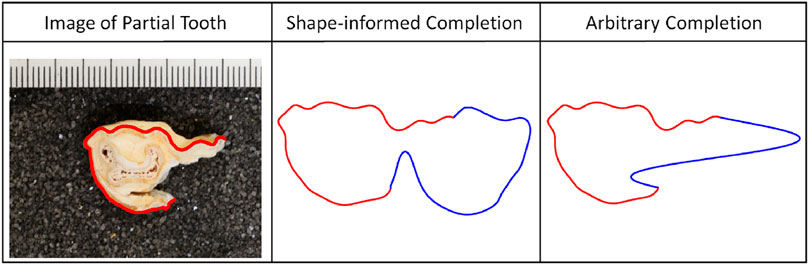
FIGURE 1. Anthropological application with bovid teeth. Left: Image of a partial tooth with the segmentation overlaid in red. Middle; Right: Shape-informed and arbitrary completions (blue) of the observed partial tooth (red), respectively.

An important consideration when considering shape of a curve is its scale. Strictly speaking, scaling a curve does not alter its shape, and it is hence a nuisance transformation. However, in our motivating application from anthropology, the size of bovid teeth is known to have important taxonomical information and can hence potentially improve discriminatory power in the classification problem [6]. We will therefore accord due consideration to scale information when comparing shapes of curves; in shape analysis vernacular, this is referred to as size-and-shape analysis. For simplicity, we will continue to chraracterize our approach as shape-informed.

Research in geometry-based statistical analysis of shapes of arbitrarily parameterized planar curves is quite mature; see, for example, [7,8] for foundational details and the R package fdasrvf for computational tools. Leveraging this, our main contributions are as follows.

1) We develop a gradient-based algorithm (Algorithm 1) for shape-informed partial matching and completion with respect to a complete template/donor curve.

2) In order to assess and visualize variability of completions from Algorithm 1, given a training dataset of fully observed curves, we propose an adaptation of the hot-deck imputation method used on traditional Euclidean data to generate several imputations or completions (Algorithm 2).

3) We propose two nearest neighbor classification procedures for partially observed curves based on shape distances by utlizing completions obtained from any of the above two algorithms.

1.1 Related Work

Partially observed curves arise as data in several applications. In medical imaging, the appearance of anatomies in images of various modalities is often summarized through the shapes of their outlines. Partial curves arise due to (i) low resolution and contrast of many medical imaging modalities (e.g., PET or CT); (ii) a boundary of an organ being obscured by other organs or hard to identify due to similar appearance of neighboring tissues [9]. In handwriting analysis, a key task is the segmentation of samples of handwriting (curves) into letters or syllables, followed by imputation of incomplete curves [10]. Shapes of occluded objects, such as tanks, are also routinely used in military applications, where only part of the object’s boundary is reliable and the rest must be imputed based on prior shape knowledge [9].

There is a substantial literature on missing data and shape analysis, however, most of the work is restricted to data obtained as multivariate morphological measurements. For example, [11] examines missing data in the morphology of crocodile skulls based on linear morphometric measurements of the skulls, in contrast to using landmarks or entire outlines (curves). Missing data methods for landmark-based shape data have been developed in [12, 13, 14, 15]. By defining landmarks on each shape, the problem can be framed in a more traditional statistical setting where each landmark can be thought of as a covariate and more traditional missing data techniques, such as the EM algorithm and multiple imputation, can be used. [16] look at four different methods for dealing with missing landmark data: Bayesian Principal Component Analysis (BPCA), least-squares regression, thin-plate splines (TPS), and mean substitution. Additional work on missing data can be found in [17], which focuses on missing data in Procrustes analysis, and [18], which considers occluded landmark data.

The work most closely related to this current study can be found in [19], which studies the problem of matching a partially observed shape to a full shape. [19] performs partial matching using the Square-Root Velocity framework, and this is the framework we use as well in the sequel. Our work in a certain sense goes beyond their work and incorporates missing data techniques into the completion procedure, and additionally is tailored towards the classification task. [9] incorporates prior shape information in Bayesian active contours that can be used to estimate object boundaries in images when the class of the object of interest is known; they demonstrate the usefulness of this approach when the object boundary is partially obscured. [20] considers the problem of identifying shapes in cluttered point clouds. They formulate a Bayesian classification model that also heavily relies on prior shape information. Finally, there is some recent work on missing data techniques for functional data analysis [21, 22, 23].

2 Shapes of Parameterized Curves

The main objects of interest in this work are parameterized curves and their shapes. Defining a suitable distance metric to compare their shapes is of fundamental importance in order to suitably formalize the notion of a “best completion of a partial curve”. From several available in the literature, we consider two distances that are suitable for our needs. We provide a description of the mathematical formulation for these two distances in the following, and refer the interested reader to [24] for more details. As discussed in the Introduction, the size of bovid teeth contains potentially taxon (class)-distinguishing information, and we hence consider the notion of size-and-shape of a curve. Throughout, for ease of exposition, we simply say shape to mean size-and-shape.

Denote by ${\mathbb{S}}^1$ the unit circle on the plane, and let $\beta :{\mathbb{S}}^1\to {\mathbb{R}}^2$ be an absolutely continuous, simple, parameterized closed curve representing the full outline of a bovid tooth. We will identify ${\mathbb{S}}^1$ with the unit interval $[\mathrm{0,1}]\subset \mathbb{R}$ and enforce the endpoint constraint β(0) = β(1) to represent a closed curve. Denote by $\mathcal{B}$ the space of all such β. If β₁ and β₂ are assumed to be parameterized according to arc-length, then $\Vert {\beta }_1-{\beta }_2\Vert ={[{\int }_0^1|{\beta }_1(t)-{\beta }_2(t){|}^2\text{d}t]}^{1/2}$ is a viable distance between them, where |⋅| is the standard Euclidean norm in ${\mathbb{R}}^2$. In order to account for nuisance information that does not alter the shape of β₁ and β₂, one must further remove variability due to translation and rotation. The two variabilities are accounted for by defining equivalence classes $[\beta ]=\{O\beta +T|O\in SO(2),T\in {\mathbb{R}}^2\}$, where SO(2) is the group of 2 × 2 rotation matrices, i.e., orthogonal matrices with determinant equal to 1. Note that the ${\mathbb{L}}^2$ distance between β₁ and β₂ is unchanged if both curves are translated and rotated by the same $T\in {\mathbb{R}}^2$ or O ∈ SO(2). Thus to compare the shapes of two curves β₁ and β₂ in $\mathcal{B}$, we can use the non-elastic shape distance

$d_{NE}\left({\beta }_1,{\beta }_2\right)=\underset{T\in {\mathbb{R}}^2,O\in SO\left(2\right)}{\min }\Vert {\beta }_1-\left(O{\beta }_2+T\right)\Vert .(1)$

This optimization problem can be solved in a straightforward fashion through Procrustes analysis [25]. The distance is termed non-elastic as it requires one to fix curve parameterizations to arc-length. Note that while d_NE is defined on $\mathcal{B}$, it is in fact a distance on the shape space ${\mathcal{S}}_{\beta }=\{[\beta ]:\beta \in \mathcal{B}\}$ of arc-length parameterized closed curves consisting of equivalence classes as points. This ensures that d_NE (β₁, β₂) = 0 if there exists $(T,O)\in SO(2)\times {\mathbb{R}}^2$ such that β₂ = Oβ₁ + T; in other words, the distance measured with d_NE is zero for two curves having the same shape.

If one desires to allow flexible parameterizations for shape analysis, the ${\mathbb{L}}^2$ metric is no longer a feasible choice as it is not invariant to re-parameterizations: ‖β₁ − β₂‖ ≠ ‖β₁◦γ − β₂◦γ‖, where $\gamma :{\mathbb{S}}^1\to {\mathbb{S}}^1$ belongs to the class Γ of orientation-preserving diffeomorphisms of ${\mathbb{S}}^1$ that represent re-parameterizations of curves in $\mathcal{B}$. When ${\mathbb{S}}^1$ is identified with [0, 1], elements of the group Γ can be viewed in the following manner. Consider the class of $\{\tilde{\gamma }:\mathbb{R}\to \mathbb{R}:\tilde{\gamma }(t+1)=\tilde{\gamma }(t)+1,\text{\hspace{0.17em}continuous\hspace{0.17em}and\hspace{0.17em}increasing}\}$. Each function in the class is such that $\tilde{\gamma }(t)-t$ is periodic with period 1. Moreover, each function of the class induces a re-parameterization ${\gamma }_s:{\mathbb{S}}^1\to {\mathbb{S}}^1$ with ${\gamma }_s(e^{2\pi it})=e^{2\pi i\tilde{\gamma }(t)}$, where $\tilde{\gamma }$ is referred to as the lift of γ_s, which is then orientation-preserving. Operationally, the construction implies that $\tilde{\gamma }$ can be expressed as $\tilde{\gamma }(t)=\gamma (t)+c$ for some γ : [0, 1] → [0, 1], which is a diffeomorphism of [0, 1], except at t = 1, and c ∈ (0, 1]. We thus construct a diffeomorphism of ${\mathbb{S}}^1$ by “unwrapping” ${\mathbb{S}}^1$ at some point s, and generating such a γ by identifying s with 0 (and 1). Henceforth, we will refer to such a γ as an orientiation-preserving reparameterization of ${\mathbb{S}}^1$, and carry out computations with [0, 1] as the parameterization domain.

Since re-parameterization completely preserves the image of a curve β, a distance based on a Riemannian metric that captures infinitesimal bending and stretching can be used. Several families of such metrics, termed as elastic have been considered [26, 27]; however, almost all of them are difficult to compute in practice and require non-trivial approximations.

A solution to this key issue was proposed in [7]. Specifically, a particular elastic metric is related to the usual ${\mathbb{L}}^2$ one when a curve is transformed bijectively to its Square-Root Velocity Function (SRVF): $\mathcal{B}\ni \beta \mapsto Q(\beta )=:q=\dot{\beta }|\dot{\beta }{|}^{-1/2}\in {\mathbb{L}}^2$, where $\dot{\beta }$ is the time-derivative. Under this transformation, ‖q₁ − q₂‖ = ‖(q₁, γ) − (q₂, γ)‖, where $(q_i,\gamma )≔(q_i◦\gamma )\sqrt{\dot{\gamma }}$ is the re-parameterization action on the SRVF. Translations are automatically removed by the use of the derivative. Let ${\mathcal{Q}}^o=\{q:[\mathrm{0,1}]\to {\mathbb{R}}^2|q\in {\mathbb{L}}^2([\mathrm{0,1}],{\mathbb{R}}^2)\}$ denote the linear space of SRVF-transformed open curves; the space of closed curve SRVFs involves an additional closure condition: $\mathcal{Q}=\{q:[\mathrm{0,1}]\to {\mathbb{R}}^2|q\in {\mathbb{L}}^2([\mathrm{0,1}],{\mathbb{R}}^2),{\int }_0^{1}q(t)|q(t)|\text{d}t=0\}$. Thus, $\mathcal{Q}$, the space of closed curve SRVFs, is a subset of ${\mathcal{Q}}^o$, the space of open curve SRVFs. We refer to [7, 24] for more details.

The corresponding elastic distance d_E between two curves ${\beta }_1,{\beta }_2\in \mathcal{B}$ is defined using their SRVFs, wherein in addition to rotations, re-parameterizations are also now optimized over:

$d_E\left({\beta }_1,{\beta }_2\right)=\underset{\left(O,\gamma \right)\in SO\left(2\right)\times \mathrm{\Gamma }}{\min }\Vert q_1-O\left(q_2◦\gamma \right)\sqrt{\dot{\gamma }}\Vert ,(2)$

where the equivalence class $[q]=\{O(q◦\gamma )\sqrt{\dot{\gamma }}|O\in SO(2),\gamma \in \mathrm{\Gamma }\}$ now represents an elastic shape, i.e., an equivalence of q under the action of SO(2) and Γ, which can be applied in any order. The optimization over SO(2) is solved via Procrustes analysis as before, while the one over Γ is addressed using Dynamic Programming or a gradient descent algorithm. This process is referred to as registration: it provides an optimal, under the elastic metric, correspondence between the shapes of q₁ and q₂. Details of computing d_E can be found in [24]. Correspondingly, define the shape space of SRVF-transformed closed curves as ${\mathcal{S}}_q=\{[q]:q\in \mathcal{Q}\}$.

In summary, if closed planar curves representing outlines of bovid teeth are assumed to be arc-length parameterized, we can use the non-elastic distance d_NE on the shape space ${\mathcal{S}}_{\beta }$ to compare their shapes. On the other hand, if the curves are allowed to have arbitrary parameterizations, it is more appropriate to consider their SRVF transforms and the shape space ${\mathcal{S}}_q$, equipped with the elastic distance d_E. Moreover, it is clear that the distances d_NE and d_E are valid for open curves as well, i.e., in the case β (0) ≠ β (1). We will use the distances for both open and closed curves without qualification; context will disambiguate their usage.

3 Partial Shape Matching and Completion

We first focus on how a single partially observed curve can be completed. Indeed, this requires a template or donor curve that is fully observed, so that the partially observed one can be matched and compared to different pieces of the fully observed one. Once a match has been established, a completion can be subsequently determined. In principle, the two tasks can be carried out sequentially or in parallel; in this paper, we adopt the former approach and leave the latter for future work.

Accordingly, the key tasks are to (i) match the observed partial curve to a piece of the donor curve; (ii) impute or complete the observed curve by finding the closest match to the residual piece of the donor curve from a set of curves with fixed endpoints. These are non-trivial tasks since the set of curves $\mathcal{B}$ (and $\mathcal{Q}$) is infinite-dimensional. The problem is made tractable by considering equivalence classes of curves that share the same shape and size, as defined earlier. Specifically, we propose to leverage the shape distances d_NE and d_E in Eqs 1, 2, and develop an optimization-based framework to carry-out completion/imputation and classification sequentially. We first define some important quantities.

• A curve β is viewed as being composed of two pieces β_o and β_m, where the subscripts o and m identify the observed and missing portions of β, such that $\beta (t)={\beta }_o(t){\mathbb{I}}_{t\in [0,\tau ]}+{\beta }_m(t){\mathbb{I}}_{t\in [\tau ,1]}$, for some 0 < τ < 1. The corresponding SRVF q similarly decomposes into (q_o, q_m) for the same τ.

• β = β_o ⋆ β_m denotes the concatenation of β_o and β_m, i.e., the complete curve. Throughout, β_o will denote a partially observed curve, which conceptually is understood to be the observed portion of a curve β; in similar fashion, β_m will throughout represent the missing piece of β.

• The restriction of a complete curve β to an open curve defined by parameter values [s₁, s₂] ⊂ [0, 1] is denoted as ${\beta }^{(s_1,s_2)}$, with its SRVF counterpart $q^{(s_1,s_2)}$ defined in a similar manner.

• Denote the length of β_o as $L({\beta }_o)={\int }_0^{\tau }|{\dot{\beta }}_o(t)|\text{d}t$, where $\dot{\beta }$ is the time-derivative. The length of the restricted curve is then $L({\beta }^{(s_1,s_2)})={\int }_{s_1}^{s_2}|{\dot{\beta }}^{(s_1,s_2)}(t)|\text{d}t$. If we fix s₁ ∈ [0, 1] and L, then s₂ ∈ [0, 1] is fully determined.

In line with our intention to use shape information of curves, we note that completion of β_o with respect to a donor curve β_donor can be broken down into the following two steps.

(i) Determine the piece of β_donor that best matches the shape of β_o.

(ii) Determine an open β_m curve that then best matches the shape of the residual piece of the donor in (i); the required completion is then β_o ⋆ β_m.

Two points are worth considering here. First, the optimal β_m is constrained to share the same endpoints as the determined piece of β_donor. Second, by virtue of its definition, the completion β_o ⋆ β_m exactly matches the partially observed curve β_o when restricted to a suitable subset of the parameter domain. The latter is motivated by the quality of image data of bovid teeth, under which it is reasonable to assume that the partially observed curve is obtained under negligible measurement error.

The key consideration for developing an algorithm for the two steps is the choice of an objective function that quantifies the quality of matches, informed by either of the shape distances d_NE and d_E in Eqs 1, 2, respectively. Repeated computation of the elastic distance d_E is computationally expensive (due to the additional optimization over Γ), and hence time-consuming inside an iterative algorithm (the potential donor set has large sample size). Since our main objective in this paper is classification of the partially observed curves, we use the more convenient non-elastic distance d_NE in order to carry out partial matching and completion. However, we will employ the elastic distance d_E when designing a classifier in order to better access pure shape features of curves that are potentially class-distinguishing.

We consider a two-step algorithm based on optimizing an objective function over two parameter spaces: Ω_P for the partial match in step (i), and Ω_C for the completion step (ii), defined as:

${\mathrm{\Omega }}_P≔\left[\mathrm{0,1}\right]\times {\mathbb{R}}^2\times SO\left(2\right)\times {\mathbb{R}}_{+}\text{and}{\mathrm{\Omega }}_C≔\left\{\beta \in \mathcal{B}|\beta \left(0\right)={\beta }_o\left(1\right),\beta \left(1\right)={\beta }_o\left(0\right)\right\}.(3)$

The parameter set Ω_P consists of shape-preserving transformations for arc-length parameterized curves β and the length of β_o, whereas Ω_C represents the subset of endpoint constrained curves within $\mathcal{B}$. In the partial matching step, a piece on the donor β_donor of optimal length L* starting at $s_1*$, rotation O* and translation T* is determined resulting in ${\beta }_{\text{donor}}^{(s_1^{*},s_2^{*})}$. The domains [s₁, s₂] of an arbitrary restriction ${\beta }_{\text{donor}}^{(s_1,s_2)}$ and [0, τ] of β_o are always rescaled to [0, 1] to ensure that they have the same domain. For a fixed s₁, the optimal translation T* and rotation O* are given explicitly via Procrustes analysis (see, for example, [28]). The search for the optimal $s_1^{*}$ and L* can then be performed exhaustively on [0, 1].

ALGORITHM 1:

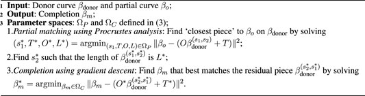
Algorithm 1:. Partial match and completion.

Note that ${\beta }_{\text{donor}}^{(s_2^{*},s_1^{*})}$ refers to the residual piece on β_donor once ${\beta }_{\text{donor}}^{(s_1^{*},s_2^{*})}$ is removed owing to the circular ordering on the parameter domain ${\mathbb{S}}^1$ of β_donor. The main challenge lies in carrying out step 3 of the algorithm in which the missing data β_m is determined by searching over ${\mathrm{\Omega }}_C\subset \mathcal{B}$ for the optimal curve that best matches the residual piece ${\beta }^{(s_2^{*},s_1^{*})}$ of β from the partial matching step. The challenge relates to the fact that Ω_C is a nonlinear subset of $\mathcal{B}$.

We propose to optimize over Ω_C with a gradient-descent algorithm. First, rescale $[s_2^{*},s_1^{*}]$ to [0, 1]. Then, consider an orthonormal basis $\{b_i:[\mathrm{0,1}]\to {\mathbb{R}}^2,i=\mathrm{1,2},\dots \}$ with b_i (0) = 0 and b_i (1) = 0, which enforce the endpoints constraint on the curve. In particular, we use a modification of the Fourier basis for each of the two coordinate functions, given by $\{\frac{\sin (2\pi jt)}{\sqrt{2}\pi j},\frac{\cos (2\pi jt)-1}{\sqrt{2}\pi j},j=\mathrm{1,2},\dots \}$¹. Let $E({\beta }_m)=\Vert (O^{*}{\beta }^{(s_2^{*},s_1^{*})}+T^{*})-{\beta }_m{\Vert }^2$. Then, the gradient of E (β_m) at a current estimate ${\beta }_m^{curr}$ can be approximated using directional derivatives along basis directions b_i as

$\nabla E\propto \sum _{i=1}^{\infty }⟨{\beta }_m^{curr}-\left(O^{*}{\beta }^{\left(s_2^{*},s_1^{*}\right)}+T^{*}\right),b_i⟩b_i,$

where ⟨⋅, ⋅⟩ is the usual ${\mathbb{L}}^2$ inner-product on $\mathcal{B}$. A single gradient update in the completion algorithm is then given by

${\beta }_m^{new}={\beta }_m^{curr}-ϵ\nabla E,$

where ϵ > 0 is a small step size. This is repeated until convergence. In practice, we reduce the dimension of the problem by truncating the basis at a finite number N; this additionally ensures that the optimal completion ${\beta }_m^{*}$ is relatively smooth. Two preliminary results from this two-step algorithm for bovid teeth are shown in Figure 2. The black curve is the donor β_donor, the red curve is β_o, and the optimal completion ${\beta }_m^{*}$, after a set number of iterations, is in blue.

FIGURE 2

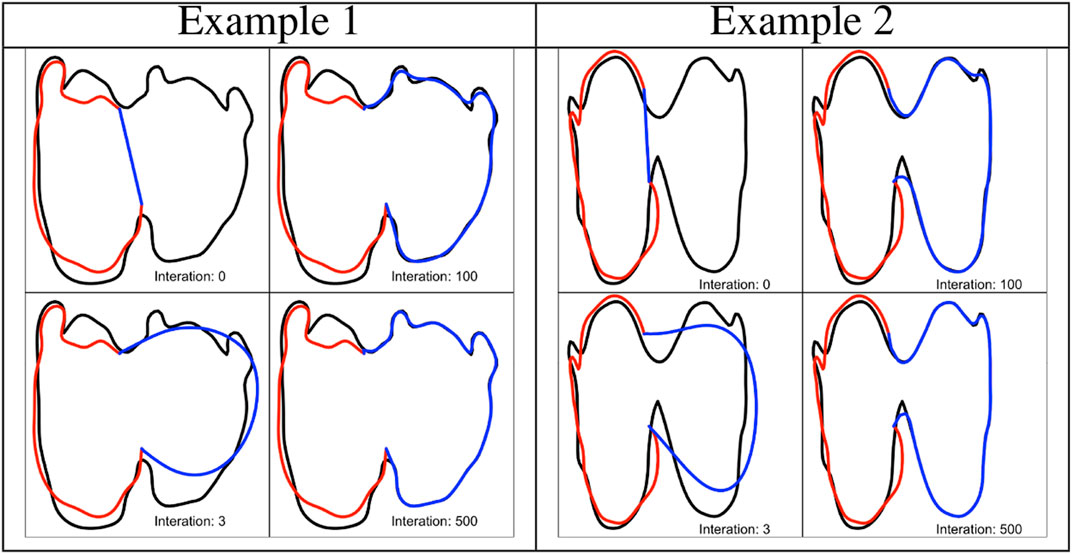
FIGURE 2. Two examples of shape imputation via Algorithm 1. The panels show the evolution of the completion (blue) at a few iterations of step 3, the observed partial curve (red) and the donor (black).

4 Assessing Variability in Completion Through Multiple Imputation

Algorithm 1 describes how a partially observed curve β_o can be completed given a donor curve β_donor. The completion is deterministic and uncertainty estimates are unavailable. Further, the application of this procedure is only possible when a training dataset consisting of several curves is available. An attractive way to examine completion variability is to consider a multiple imputation framework for missing data. There are numerous multiple imputation methods to handle missing data in traditional multivariate settings; see [29, 30] for a broad overview and details on missing data techniques. Our choice is a nonparametric hot-deck multiple imputation procedure. We describe this technique in a regression setting with response $\mathit{y}\in {\mathbb{R}}^n$ and n × p design matrix X, where each case j = 1, … , n is defined as the response-predictor pair (y_j, x_j).

(i) Replace a missing value y_miss of y with randomly selected observed values in y, chosen from a donor pool of fixed size K < n comprising fully observed cases that are“similar” to the incomplete case.

(ii) Repeat step (i) M times to create M completed datasets.

(iii) Analyze the M completed datasets independently (e.g., mean estimation) and combine results using Rubin’s combining rules [29].

As a first step towards carrying out this program for partially observed curves, we propose an adaptation of the hot-deck imputation procedure for a classification task. However, the development of methods to combine classification results across M datasets, similar to Rubin’s rules, is an interesting research problem in its own right, and we leave that for future work (Section 7). Once steps (i) and (ii) are completed, it is possible to visualize variability associated with completion using Algorithm 1 by plotting the completions. Moreover, variability in classification results can also be computed as a function of a donor set of size K and number of completed datasets M. Algorithm 2 outlines our adapted hot-deck imputation procedure for generating M completions of a partially observed curve β_o given a training dataset $\mathcal{D}=\{{\beta }_1,\dots ,{\beta }_n\}$ consisting of n fully observed curves from $\mathcal{B}$. The main change to the classic hot-deck imputation procedure described above lies in how “similarity” between cases (here curves) is assessed in (i). In particular, steps 3–8 in Algorithm 2 are used to compute the (shape) similarity between a partially observed curve and each curve in the training dataset $\mathcal{D}$. Then, the rest of (i) is carried out in step 9. Finally, (ii) is carried out in steps 10–13.

ALGORITHM 2:

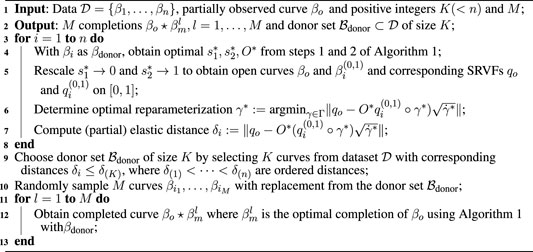
Algorithm 2:. Hot-deck imputation.

Note that once $s_1^{*}$ and $s_2^{*}$ are rescaled to 0 and 1, respectively, in line 5, the optimal partial match of β_i to β_o then corresponds to the piece ${\beta }_i^{(\mathrm{0,1})}$ of length L* from β_i, which is now represented as an open curve ${\beta }_i^{(\mathrm{0,1})}:[\mathrm{0,1}]\to {\mathbb{R}}^2$; the parameter domain [0, 1] of ${\beta }_i^{(\mathrm{0,1})}$ is not to be confused with the parameter [0, 1], representing ${\mathbb{S}}^1$, of the fully observed curve β_i. Similar comments apply to their corresponding SRVF versions. Note and contrast step 7 of Algorithm 2 to the completion step 3 in Algorithm 1: here, the distance δ_i is computed between β_o and the matched piece of the donor, and not the residual piece.

The key feature of Algorithm 2 is the use of the elastic distance, albeit not exactly in the form defined in (2) since an optimal rotation O* ∈ SO(2) has already been determined in line 5–we hence refer to this distance as partial elastic distance. The rationale for this is as follows. Once a piece of the donor β_i of length L* corresponding to parameter values $s_1^{*}$ and $s_2^{*}$ has been extracted, the lengths of ${\beta }_i^{(s_1^{*},s_2^{*})}$ and β_o can be quite different. Thus, computing the non-elastic distance between the two open curves under the assumption of arc-length parameterization in order to compare their shapes might not be appropriate. In contrast, in Algorithm 1, the distances themselves were not of chief interest. Our approach hence is to assume at this stage that ${\beta }_i^{(s_1^{*},s_2^{*})}$ and β_o are arbitrarily parameterized and hence use the partial elastic distance d_E to compare their shapes using their corresponding SRVFs; this also explains why we ignore using the optimal translation T* resulting from Algorithm 1. To see that δ_i in line 8 of Algorithm 2 is indeed the partial shape distance, note that when a particular rotation O* is fixed, from line 6

$\underset{\gamma \in \mathrm{\Gamma },O\in SO\left(2\right)}{\inf }\Vert q_0-O^{*}\left(q_i^{\left(\mathrm{0,1}\right)}◦\gamma \right)\sqrt{\dot{\gamma }}\Vert =\underset{\gamma \in \mathrm{\Gamma }}{\inf }\Vert q_0-O^{*}\left(q_i^{\left(\mathrm{0,1}\right)}◦\gamma \right)\sqrt{\dot{\gamma }}\Vert =\Vert q_o-O^{*}\left(q_i^{\left(\mathrm{0,1}\right)}◦{\gamma }^{*}\right)\sqrt{{\dot{\gamma }}^{*}}\Vert .$

Figure 3 provides an illustration of the hot-deck imputation procedure with M = 10 and K = 10 for two partially observed bovid teeth using Algorithm 2; see Section 6 for details on the bovid dataset.

FIGURE 3

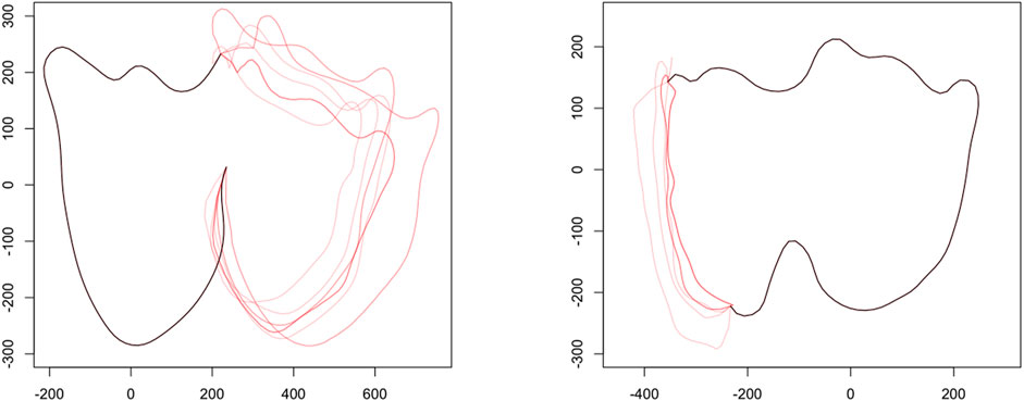
FIGURE 3. Examples of partial matches followed by imputation on partially observed teeth. Left: Approximately 50% of the tooth is observed. Right: Approximately 80% of the tooth is observed. The black curve denotes the fully observed portion of the tooth with each red curve being a single completion of the tooth. In both examples shown here M = 10 and K = 10.

5 Nearest Neighbor Classification

Consider a training dataset ${\mathcal{D}}_{\text{train}}≔{\{(y_i,{\beta }_i)\}}_{i=1}^n$ consisting of fully observed curves ${\beta }_i\in \mathcal{B}$ and corresponding class labels y_i ∈ {1, … , G}. The goal is to classify a partially observed curve β_o to one of the G classes using training data ${\mathcal{D}}_{\text{train}}$.

A distance-based classification procedure is a natural choice, compatible with how completion and imputation is achieved. Accordingly, we consider the k_n-nearest neighbor classification technique. A neighborhood of a curve in $\mathcal{B}$ can be defined with respect to both non-elastic and elastic shape distances d_NE and d_E. Effectively, although fully observed curves in ${\mathcal{D}}_{\text{train}}$ assume values in $\mathcal{B}$, the classification procedure will be defined on their shapes assuming values in the shape space ${\mathcal{S}}_{\beta }$ (or ${\mathcal{S}}_q$ under the SRVF transform).

The advantage of using the shape space lies in the fact that ${\mathcal{S}}_{\beta }$ is made up of equivalence classes of $\mathcal{B}$ under the equivalence relation characterized by shape-preserving transformations. For a fixed radius r, neighborhoods as balls of radius r around a fixed point β* constructed on $\mathcal{B}$ using shape distances d_NE are necessarily larger than corresponding ones on $\mathcal{B}$ using the usual ${\mathbb{L}}^2$ distance, since, by virtue of its definition, for every r > 0,

$\left\{\beta \in \mathcal{B}:\Vert \beta -{\beta }^{*}\Vert \le r\right\}\subseteq \left\{\beta \in \mathcal{B}:d_{NE}\left(\beta ,{\beta }^{*}\right)\le r\right\}.$

In a k_n-nearest neighbor setting, the radius r is distance, say $r_{k_n}$, of the $k_n^{\mathsf{t}\mathsf{h}}$ closest curve to β*, and changes with the training data. However, $r_{k_n}$ computed using the distance d_NE will be smaller than one computed using the ${\mathbb{L}}^2$ distance; thus one is able to find k_n neighbors at a smaller distance from β*. This leads to better performance of the classifier for large sample size n and improves rates of convergence of the predicted class probabilities (see, for example, [31]). Similar comments apply to the elastic distance d_E, albeit under subtler conditions since it is induced by the elastic Riemannian metric on $\mathcal{B}$, which is not directly related to the ${\mathbb{L}}^2$ metric on $\mathcal{B}$.

We will use the elastic distance d_E again to accommodate for the possibility that curves in ${\mathcal{D}}_{\text{train}}$ and β_o ⋆ β_m can have arbitrary parameterizations following completion of β_o with any β_m. Let ${\mathcal{N}}_{k_n}({\beta }_o\star {\beta }_m)≔\{{\beta }_{i_1},\dots ,{\beta }_{i_{k_n}}\}\subset {\mathcal{D}}_{\text{train}}$ be k_n nearest curves to a particular completion β_o ⋆ β_m of β_o in the training data. We consider two nearest neighbor classifiers.

• knn classifier: Assign β_o to the class with largest predicted probability. The predicted probability that label y for β_o assumes value g ∈ {1, … , G} is given by

$\pi \left(y=g|{\beta }_o,{\mathcal{D}}_{\text{train}}\right)=\frac{1}{k_n}\sum _{{\beta }_i\in {\mathcal{N}}_{k_n}\left({\beta }_o\star {\beta }_m\right)}{\mathbb{I}}_{\left\{y_i=g\right\}},$

 and β_o ⋆ β_m is one completion obtained from Algorithm 1 with β_m ∈ Ω_C.

• knn-imp classifier: Here, we incorporate uncertainty in completion of β_o into the classification procedure by combining the knn classifier with hot-deck imputation. Specifically, with M completions ${\beta }_o\star {\beta }_m^l,l=1,\dots ,M$ obtained from Algorithm 2, the corresponding class probability is

$\pi \left(y=g|{\beta }_o,{\mathcal{D}}_{\text{train}}\right)=\frac{1}{k_{n}M}\sum _{l=1}^M\sum _{{\beta }_i\in {\mathcal{N}}_{k_n}\left({\beta }_o\star {\beta }_m^l\right)}{\mathbb{I}}_{\left\{y_i=g\right\}}.$

The class probability is thus obtained by averaging over all completions obtained by sampling M donor curves with replacement from the donor set ${\mathcal{B}}_{\text{donor}}$ in Algorithm 2.

The knn-imp classifier is a novel extension of the knn classifier to accommodate variability in completions through the hot-deck multiple imputation procedure. However, at the outset, it is not clear if it will generally outperform the knn classifier, since performance will heavily depend on quality of the completion step in Algorithm 1 and shape variability in the training dataset.

6 Tribe and Species Classification of Bovid Teeth

We examine performance of Algorithm 1 and Algorithm 2 with respect to classification of images of fully and partially observed bovid teeth using the two nearest neighbor methods under two settings.

(i) A simulated setting, where curves pertaining to partially observed teeth are created from fully observed ones with known class labels.

(ii) A real data setting comprising “true” partially observed teeth with unknown class labels.

There are numerous measures of classification performance. We use the log-loss measure to asses performance: let n_p denote the number of partially observed curves ${\beta }_o^1,\dots ,{\beta }_o^{n_p}$ to be classified in G classes {1, … , G} with unknown class labels $y_1,\dots ,y_{n_p}$ and let ${\mathcal{D}}_{\text{train}}$ denote the training dataset of fully observed curves. Then

$\text{Log}-\text{loss}≔-\frac{1}{n_p}\sum _{i=1}^{n_p}\sum _{g=1}^G{\mathbb{I}}_{\left\{y_i=g\right\}}\log \left[\pi \left(y_i=g|{\beta }_o^i,{\mathcal{D}}_{\text{train}}\right)\right],$

where the class probability is defined as earlier depending on whether the knn or knn-imp classifier is used. Evidently, a low Log-loss is indicative of good classification. Note that the Log-loss is positive with no upper bound. The Log-loss can be used only when the class labels are known. In the real data setting with unknown labels, the Log-loss is not used; instead, classification accuracy is assessed relative to classification done by an expert (co-author JKB).

All computations are performed using routines available in the R [32] package fdasrvf [33] on a 16-node Intel Xeon-based computational cluster in the Computer Science Department at Loyola University Chicago. Full code for the analyses can be found on Github [34].

Our motivating application stems from anthropology, where fossil bovid teeth associated with our human ancestors are used to reconstruct past environments. Bovids are useful because they are ecologically sensitive to their environment and typically dominate the South African faunal assemblages [35, 36, 37, 38].

The tooth images for our study were obtained from four institutions in South Africa: National Museum, Bloemfontein; Ditsong Museum, Pretoria; and Amathole Museum, King William’s Town. Images were also taken at the Field Museum, Chicago, United States. The complete methodology as to how the teeth images were collected is outlined in [6]. Briefly, the occlusal surface of each of the three molars from the upper and lower dentitions for each extant bovid specimen were photographed separately. The specimen and the camera were levelled using a bubble level. A scale was placed next to the occlusal surface for every image.

Specifically, we consider images of teeth from 7 bovid tribes (Alcelaphini, Antilopini, Bovini, Hippotragini, Neotragini, Reduncini, and Tragelaphini) and 20 species (R. arundinum, A. buselaphus, S. caffer, R. campestris, P. capreolus, D. dorcas, K. ellipsiprymnus, H. equinus, R. fulvorufula, O. gazella, C. gnou, K. leche, A. marsupialis, H. niger, O. oreotragus, T. oryx, O. ourebi, T. scriptus, T. strepsiceros, C. taurinus). The dataset contains six tooth types: lower (i.e., mandibular) molars 1, 2 and 3 (LM1, LM2, LM3), and upper (i.e., maxillary) molars 1, 2 and 3 (UM1, UM2, UM3). Specific counts of the sample sizes of each tooth type and tribe are in Table 1. This dataset contains fully observed teeth of known taxa and will constitute the training data ${\mathcal{D}}_{\text{train}}$.

TABLE 1

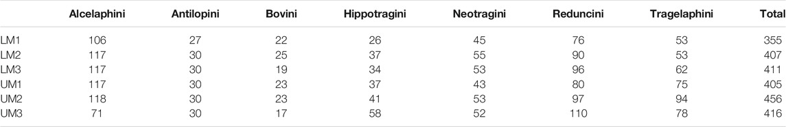
TABLE 1. Sample sizes for each tooth type and tribe.

Each tribe has unique dental characteristics that are shared by its members. Further, the complexity of the occlusal surface outline varies across the tribes. As such, considering shape for tribe classification is a natural endeavor in this application. Generally, classification at the species level is more difficult since the variability of shapes of occlusal surface outlines across species within the same tribe is not as large.

6.1 Simulated Setting

In this setting, a partially observed tooth was created from a fully observed one with known class label in ${\mathcal{D}}_{\text{train}}$, and a class probability is calculated using both nearest neighbor methods; the procedure is repeated for each tooth in ${\mathcal{D}}_{\text{train}}$ and the Log-loss is computed for the knn and knn-imp classifiers for choices:

(i) K = 5, 10, 20 of size of donor set ${\mathcal{B}}_{\text{donor}}$;

(ii) M = 5, 10, 20 of number of imputations based on sampling with replacement from ${\mathcal{B}}_{\text{donor}}$;

(iii) k_n = 1, 2, … , 20 of number of neighbors;

(iv) Tooth types LM1, LM2, LM3, UM1, UM2 and UM3;

(v) Side of tooth extracted, where Left is denoted as 1 and Right as 2.

A partially observed tooth was created in the following manner. The raw representation of each tooth in ${\mathcal{D}}_{\text{train}}$ comprised of 60 points around the occlusal surface of the tooth that were obtained from the program MLmetrics [6, 39]. For each tooth, the 60 points were split into two sets roughly divided by a line connecting the mesostyle to the entostyle in maxillary teeth and metastylid to the ectostylid in mandibular teeth. This type of cut was chosen as this break point is commonly observed in fossilized bovid teeth. Figure 4 provides an illustrative example of the procedure.

FIGURE 4

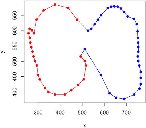
FIGURE 4. An example of how a partially observed tooth is obtained from a fully observed one in the simulated setting. The figure shows a lower molar 1 (LM1) from the tribe Alcelaphini with red points representing the extracted piece from the Left (1) side and blue points do the same for the Right (2) side.

6.1.1 Tribe classification

Figure 5 shows Log-loss curves associated with the knn-imp classifier as a function of k_n (number of neighbors) for the above-mentioned choices of M and K, and also the corresponding curve for the knn classifier. In all cases, for smaller values of the number of nearest neighbors chosen, the knn-imp classifier outperforms the knn classifier. As the number of nearest neighbors increases, not performing imputation performs as well or better than imputation in most cases. In fact, for some teeth there are certain combinations of M and K that are better in terms of Log-loss for imputation regardless of the choice k_n of nearest neighbors.

FIGURE 5

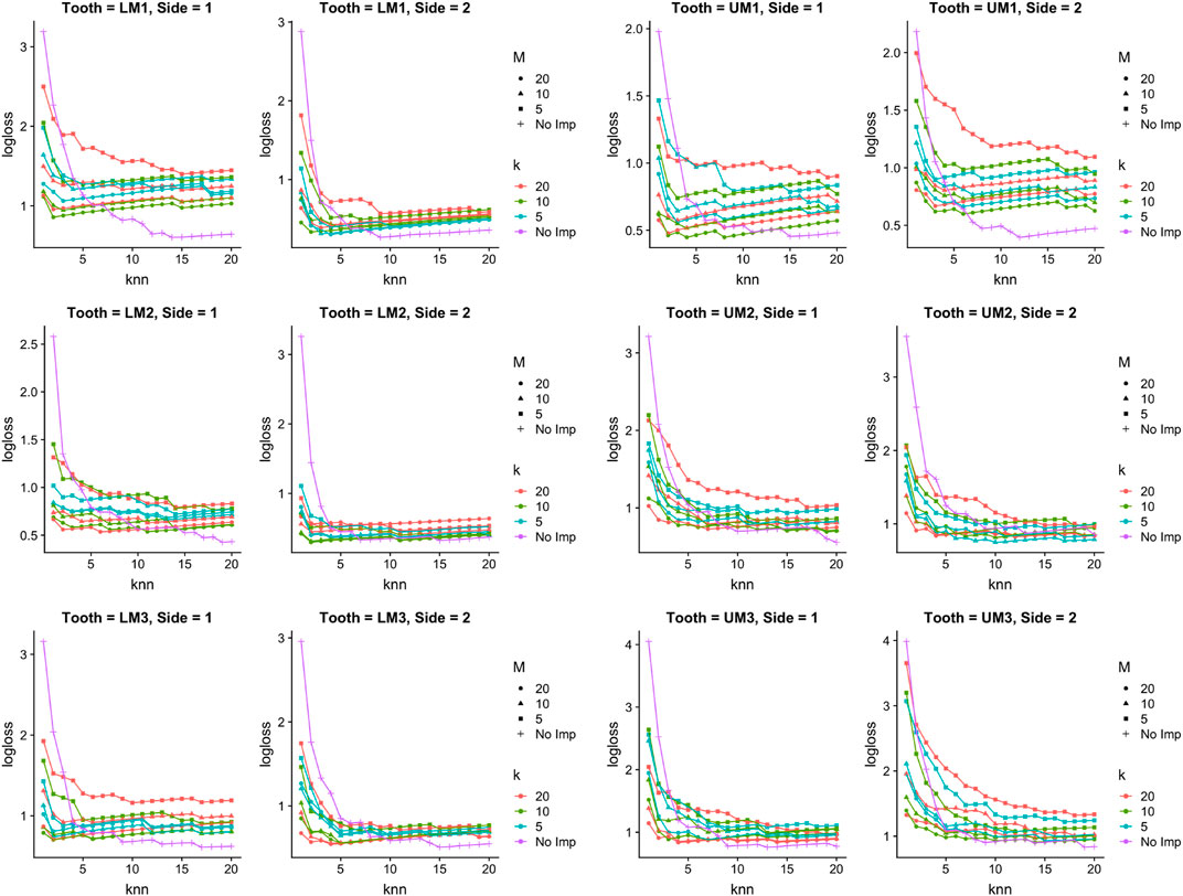
FIGURE 5. Tribe classification in simulated setting. Log-loss for the knn-imp classifier as a function of number k_n neighbors for different values of donor set size K and number of imputations M; purple “No-imp” curve represents the same for the knn classifier.

6.1.2 Species classification

Figure 6 shows Log-loss curves for species classification and paints a fairly similar picture to Figure 5: when the number of nearest neighbors is chosen to be small (i.e., fewer than 5), there is always at least one imputation setting that has lower Log-loss than no imputation. However, in all cases as the number of nearest neighbors chosen gets close to 20, no imputation performs better in terms of Log-loss than doing imputation.

FIGURE 6

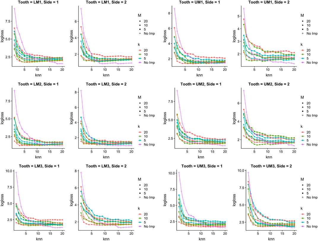
FIGURE 6. Species classification in simulated setting. Log-loss for the knn-imp classifier as a function of number k_n neighbors for different values of donor set size K and number of imputations M; purple “No-imp” curve represents the same for the knn classifier.

6.2 Real Data Setting

A small set n_p = 7 of real, partially observed fossil bovid teeth from the site of Gladysvale, South Africa, extracted from images, with unknown class labels were used. We use the image numbers to label them: IMG4825, IMG4980, IMG4983, IMG4990, IMG5139, IMG9973 and IMG5514. Training data ${\mathcal{D}}_{\text{train}}$ is the same as the one used in the simulated setting. Recall that in the simulation setting, partially observed teeth had roughly half of the number of sampled points as the fully observed ones. In the real data setting, this is not the case: in four partially observed teeth (IMG4825, IMG4980, IMG4983, IMG9973), more than half of the tooth is observed; in one (IMG4990) less than half of the tooth is observed; and, in the remaining two (IMG5139, IMG5514), approximately half of the tooth is observed. This impacts the number of points chosen to represent (and parametrize) the open, partially observed curves. Since we cannot know the length of the missing piece for real partially observed curves, numbers of points to sample along the curves were determined based on expert advice from co-author JKB.

For both knn-imp and knn classifiers, we set the number of neighbors k_n = 10; for the knn-imp classifier we used K = 10 and M = 10. These choices were based on performances in the simulated setting.

6.2.1 Classification at Tribe Level

Table 2 shows predicted class probabilities associated with the knn classifier. Each row has an entry in bold indicating the “true” (according to an expert) class of these teeth. We observe that the classifications without imputation are highly accurate for the 7 teeth. One can see that 6 out of 7 of these teeth are classified to the correct tribe. In addition, the probability of belonging to the correct tribe in the 6 correctly classified teeth was 1. However, in the one case where the classification is wrong, the predicted probability was 0.

TABLE 2

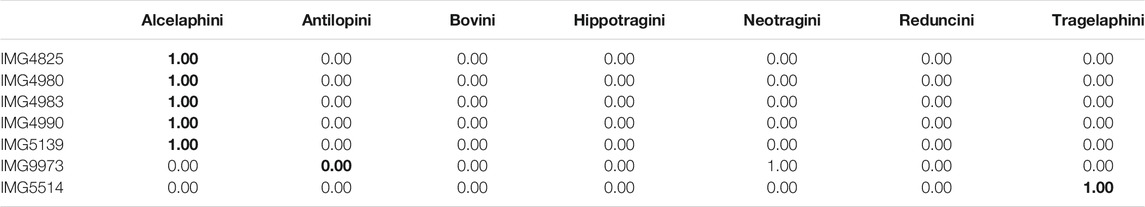
TABLE 2. Real data. Tribe level predicted class probabilities from the knn classifier with k_n = 10. Emboldened values indicate the “true” class as obtained from an expert.

Table 3 shows similar results for the knn-imp classifier. The same 6 teeth that were correctly classified before are again correctly classified, however, with probabilities that are all lower than 1. Again, the tooth that was incorrectly classified previously is again incorrectly classified and the probability predicted of belonging to the correct class is again 0. Notably, the partially observed tooth from IMG9973 was difficult to classify when using either classifier; interestingly, in both cases it was classified with high probability to the Neotragini class.

TABLE 3

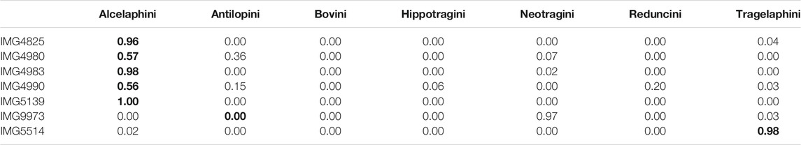
TABLE 3. Real data. Tribe level predicted class probabilities from the knn-imp classifier with k_n = K = M = 10. Emboldened values indicate the “true” class as obtained from an expert.

6.2.2 Classification at the Species Level

Table 4 shows predicted class probabilities associated with the knn classifier. We saw in Tables 2, 3 that each of the 5 teeth from the Alcelaphini tribe was correctly classified, with probability at least 0.5. However, at the species level, only 2 of these 5 teeth (IMG4983, IMG4990) have high probability associated with the correct species; the three other teeth (IMG4825, IMG4980 and IMG5139) have a probability of belonging to the correct species of 0.4. In addition, for the two remaining teeth that belong to the Tragelaphini and Antilopini tribes, the predicted probability for the correct species was 0.1 and 0, respectively.

TABLE 4

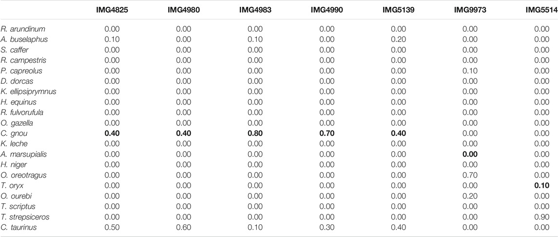
TABLE 4. Real data. Species level predicted class probabilities with knn classifier with k_n = 10. Emboldened values indicate the “true” class as obtained from an expert.

When classifying using the knn-imp classifier with imputation, the results are similar with a few notable differences. Table 5 shows these results. First, of the 5 Alcelaphini teeth, 3 are correctly classified using imputation (IMG4825, IMG4990 and IMG5139). Second, two of these are in fact correctly classified with higher probability when carrying out imputation with the knn-imp classifier when compared to the knn classifier (IMG4825: 0.44 vs. 0.4 and IMG5129: 0.52 vs. 0.4). Finally, the other four teeth corresponding to IMG4980, IMG4983, IMG9973 and IMG5514 had predicted probabilities for the correct species of 0.04, 0.22, 0 and 0.09, respectively.

TABLE 5

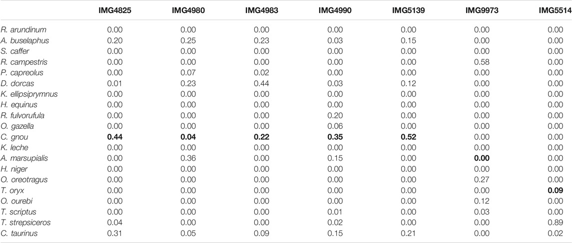
TABLE 5. Real data. Species-level predicted class probabilities with knn-imp classifier with k_n = K = M = 10. Emboldened values indicate the “true” class as obtained from an expert.

7 Discussion

We have presented a computational approach for classifying partially observed curves. In particular, we presented two algorithms to complete and classify partially observed planar curves and simultaneously assess variability involved with the completion through a multiple imputation procedure. To our knowledge, this is the first work in literature to explicitly use the notion of shapes of parameterized curves in addressing the problem considered from the missing data perspective; coarsening the parameter space of suitable open curves, from which the partially observed curves are completed, through the notion of shape equivalence results in sensible completions. Moreover, shape-based distances used to define classifiers deliver satisfactory classification performance. The results from application of the algorithms to the dataset of images of bovid teeth are quite promising and are deserving of further, extensive, investigation involving several different classifiers.

Through the application of the proposed framework on real data, we have found that hot-deck imputation can sometimes deteriorate classification performance; there is an intuitive explanation for these findings. Classification performance is greatly affected by the “amount of information” contained in the observed partial curve. By “amount of information”, we specifically mean the ability to discriminate between different classes. In particular, if the observed partial curve contains a lot of information about its class membership compared to the missing portion, then imputation injects additional variability into the problem, which has a negative effect on classification performance. On the other hand, if the observed partial curve is not easily distinguishable across the different classes in the training data, then the variability coming from the imputation procedure provides valuable information, thus improving classification performance. Knowledge about information content in an observed partial curve for classification can be obtained either from a training dataset consisting of fully observed curves with class labels or from a subject matter expert. In such cases, a Bayesian classification model with a judicious choice of prior on class-specific templates can be developed; such an approach will extend the one recently proposed for univariate functional data [23] to the curve setting, and constitutes ongoing work.

As with any methodological development that represents a first foray into tackling a challenging problem, our approach suffers from a few shortcomings, which inevitably present many possible avenues for future research. Algorithm 1 can be improved. Ideally, the partial match and completion steps are carried out jointly. Moreover, assuming curves to be arc-length parameterized, while convenient, can sometimes be unrealistic in practice, especially when data curves are extracted as part of an elaborate pre-processing procedure. This points towards developing a version of Algorithm 1 based on the corresponding SRVFs q_o and q_m; the main challenge here is how to handle the interplay between points $\{s_1^{*},s_2^{*}\}$ and their images $\{\gamma (s_1^{*}),\gamma (s_2^{*})\}$ under arbitrary reparameterizations.

In the current work, an explicit statistical model to handle the several sources of variation (e.g., measurement error in extracting curves from images) that can profoundly affect both completion and classification is conspicuous in its absence; without such a model, it is difficult to quantify uncertainty about the completions, which quite naturally percolates down to the classification task. An attractive model-based approach is to not just estimate the missing piece of the partially observed curve, but instead estimate an entire template that has a portion that is very similar in shape to the partially observed curve. Such an approach has recently been used for traditional univariate functional data under a Bayesian formulation [23] and appears promising.

Our primary task in this paper is classification. However, it is unclear how one can use the proposed algorithms if interest was in computing statistical summaries in the presence of partially observed curves, such as the mean shape or PCA on the space of shapes. For example, output of Algorithm 2 is a set of M closed curves ${\beta }_o\star {\beta }_m^l, l=1,\dots ,M$ with the property that each ${\beta }_o\star {\beta }_m^l$ exactly matches β_o on a subset of the parameter domain; it is not clear how the M completions can be combined (e.g., a Karcher mean of closed curves) to construct a representative summary completion. This is related to how estimates from imputations can be combined with a handle on within and across sample variabilities using formal rules (e.g., Rubin’s rules). Development of such general rules in the present setting is far from straightforward.

More generally, while the hot-deck imputation procedure worked reasonably well when combined with the completion task, there is a pressing need to systematically develop missing data concepts and imputation methods to better address the special structure of missingness in the context of shapes of curves. The following challenges naturally arise: (i) Is the notion of Missing Completely at Random (MCAR), so profitably used in traditional settings, ever a reasonable assumption for shapes of curves? It is almost impossible to disentangle measurement error from reasons for why a piece of a curve is missing. (ii) Conditional probability measures associated with random functions when conditioned on its values in a sub-domain are notoriously difficult, and rarely exist. Given this, how does one adapt, or perhaps circumvent, the traditional notion of sampling from the conditional distribution of the missing values conditioned on the observed values to the present setting? Much remains to be done in this direction.

Data Availability Statement

The raw data supporting the conclusions of this article will be made available by the authors, without undue reservation.

Author Contributions

All authors participated in problem formulation. GM, KB, SK, and OH developed and implemented the methodology. GM analyzed the data. JB provided the data and interpreted the results. GT helped with computation.

Funding

This work is partially supported by the following grants: NSF DMS-2015320, NSF DMS-1811969 (OH); NSF DMS-1812065, NSF DMS-2015236 (JKB); NSF DMS-1812124 (GJM and GKT); NSF DMS- 2015374 (GJM and KB); NSF NIH R37-CA214955 (SK and KB); EPSRC EP/V048104/1 (KB); NSF CCF-1740761, NSF DMS-2015226, NSF CCF-1839252 (SK).

Conflict of Interest

The authors declare that the research was conducted in the absence of any commercial or financial relationships that could be construed as a potential conflict of interest.

Publisher’s Note

All claims expressed in this article are solely those of the authors and do not necessarily represent those of their affiliated organizations, or those of the publisher, the editors and the reviewers. Any product that may be evaluated in this article, or claim that may be made by its manufacturer, is not guaranteed or endorsed by the publisher.

Acknowledgments

We thank Professor Ian Jermyn for valuable discussions on this topic. We would also like to thank Grady Flanary and Kajal Chokshi for their help in the early stages of this project.

Footnotes

¹In practice, the basis is truncated to some finite number. We have found that between 40 and 80 total basis elements per coordinate function are sufficient, although this depends on the geometric complexity of the observed curves. In the application considered in Section 6, we used 80 basis elements.

References

1. Delaigle, A, and Hall, P. Classification using censored functional data. J Am Stat Assoc (2013) 108(504):1269–83. doi:10.1080/01621459.2013.824893

CrossRef Full Text | Google Scholar

2. Delaigle, A, and Hall, P. Approximating fragmented functional data by segments of Markov chains. Biometrika (2016) 103:779–99. doi:10.1093/biomet/asw040

CrossRef Full Text | Google Scholar

3. Descary, M-H, and Panaretos, VM. Recovering covariance from functional fragments. Biometrika (2018) 106(1):145–60. doi:10.1093/biomet/asy055

CrossRef Full Text | Google Scholar

4. Lin, Z, Wang, J-L, and Zhong, Q. Basis expansions for functional snippets. Oxford: Biometrika (2020). In Press.

Google Scholar

5. Kraus, D. Components and completion of partially observed functional data. J R Stat Soc B (2015) 77(5):777–801. doi:10.1111/rssb.12087

CrossRef Full Text | Google Scholar

6. Brophy, JK, de Ruiter, DJ, Athreya, S, and DeWitt, TJ. Quantitative morphological analysis of bovid teeth and implications for paleoenvironmental reconstruction of Plovers Lake, Gauteng Province, South Africa. J Archaeological Sci (2014) 41:376–88. doi:10.1016/j.jas.2013.08.005

CrossRef Full Text | Google Scholar

7. Srivastava, A, Klassen, E, Joshi, SH, and Jermyn, IH. Shape analysis of elastic curves in Euclidean spaces. IEEE Trans Pattern Anal Mach Intell (2011) 33:1415–28. doi:10.1109/tpami.2010.184

PubMed Abstract | CrossRef Full Text | Google Scholar

8. Kurtek, S, Srivastava, A, Klassen, E, and Ding, Z. Statistical modeling of curves using shapes and related features. J Am Stat Assoc (2012) 107(499):1152–65. doi:10.1080/01621459.2012.699770

CrossRef Full Text | Google Scholar

9. Joshi, SH, and Srivastava, A. Intrinsic Bayesian active contours for extraction of object boundaries in images. Int J Comput Vis (2009) 81(3):331–55. doi:10.1007/s11263-008-0179-8

CrossRef Full Text | Google Scholar

10. Kurtek, S, and Srivastava, A. Handwritten text segmentation using elastic shape analysis. In: International Conference on Pattern Recognition (2014). p. 2501–6. doi:10.1109/icpr.2014.432

CrossRef Full Text | Google Scholar

11. Brown, CM, Arbour, JH, and Jackson, DA. Testing of the effect of missing data estimation and distribution in morphometric multivariate data analyses. Syst Biol (2012) 61(6):941–54. doi:10.1093/sysbio/sys047

PubMed Abstract | CrossRef Full Text | Google Scholar

12. Gunz, P, Mitteroecker, P, Neubauer, S, Weber, GW, and Bookstein, FL. Principles for the virtual reconstruction of hominin crania. J Hum Evol (2009) 57:48–62. doi:10.1016/j.jhevol.2009.04.004

PubMed Abstract | CrossRef Full Text | Google Scholar

13. Gunz, P, Mitteroecker, P, Bookstein, FL, and Weber, GW. Computer-aided reconstruction of incomplete human crania using statistical and geometrical estimation methods. In: Enter the past: the e-way into the four dimensions of cultural heritage; CAA 2003; computer applications and quantitative methods in archaeology. Oxford: Archaeopress (2004). p. 92–4.

Google Scholar

14. Neeser, R, Ackermann, RR, and Gain, J. Comparing the accuracy and precision of three techniques used for estimating missing landmarks when reconstructing fossil Hominin Crania. Am J Phys Anthropol (2009) 140:1–18. doi:10.1002/ajpa.21023

PubMed Abstract | CrossRef Full Text | Google Scholar

15. Couette, S, and White, J. 3D geometric morphometrics and missing-data. Can extant taxa give clues for the analysis of fossil primates? Gen Palaeontology (2009) 9:423–33.

Google Scholar

16. Arbour, JH, and Brown, CM. Incomplete specimens in geometric morphometric analyses. Methods Ecol Evol (2014) 5:16–26. doi:10.1111/2041-210x.12128

CrossRef Full Text | Google Scholar

17. Albers, CJ, and Gower, JC. A general approach to handling missing values in procrustes analysis. Adv Data Anal Classif (2010) 4(4):223–37. doi:10.1007/s11634-010-0077-0

CrossRef Full Text | Google Scholar

18. Mitchelson, JR. MOSHFIT: algorithms for occlusion-tolerant mean shape and rigid motion from 3D movement data. J Biomech (2013) 46:2326–9. doi:10.1016/j.jbiomech.2013.05.029

PubMed Abstract | CrossRef Full Text | Google Scholar

19. Robinson, DT. Functional Data Analysis and Partial Shape Matching in the Square Root Velocity Framework. PhD thesis. Florida: Florida State University (2012).

Google Scholar

20. Srivastava, A, and Jermyn, IH. Looking for Shapes in Two-Dimensional Cluttered Point Clouds. IEEE Trans Pattern Anal Mach Intell (2009) 31(9):1616–29. doi:10.1109/tpami.2008.223

PubMed Abstract | CrossRef Full Text | Google Scholar

21. Liebl, D, and Rameseder, S. Partially observed functional data: The case of systematically missing parts. Comput Stat Data Anal (2019) 131:104–15. doi:10.1016/j.csda.2018.08.011

CrossRef Full Text | Google Scholar

22. Ciarleglio, A, Petkova, E, and Harel, O. Elucidating age and sex-dependent association between frontal EEG asymmetry and depression: An application of multiple imputation in functional regression. J Am Stat Assoc (2021). In Press. doi:10.1080/01621459.2021.1942011

CrossRef Full Text | Google Scholar

23. Matuk, J, Bharath, K, Chkrebtii, O, and Kurtek, S. Bayesian framework for simultaneous registration and estimation of noisy, sparse and fragmented functional data. J Am Stat Assoc (2021). In Press, doi:10.1080/01621459.2021.1893179

CrossRef Full Text | Google Scholar

24. Srivastava, A, and Klassen, EP. Functional and Shape Data Analysis. New York, NY: Springer (2016).

Google Scholar

25. Kendall, DG. Shape Manifolds, Procrustean Metrics, and Complex Projective Spaces. Bull Lond Math Soc (1984) 16:81–121. doi:10.1112/blms/16.2.81

CrossRef Full Text | Google Scholar

26. Younes, L. Computable Elastic Distances between Shapes. SIAM J Appl Math (1998) 58(2):565–86. doi:10.1137/s0036139995287685

CrossRef Full Text | Google Scholar

27. Mio, W, Srivastava, A, and Joshi, S. On shape of plane elastic curves. Int J Comput Vis (2007) 73(3):307–24. doi:10.1007/s11263-006-9968-0

CrossRef Full Text | Google Scholar

28. Dryden, IL, and Mardia, KV. Statistical Shape Analysis. Chichester: John Wiley & Sons (1998).

Google Scholar

29. Little, RJA, and Rubin, DB. Statistical Analysis with Missing Data. UK: John Wiley & Sons (1987).

Google Scholar

30. Andridge, RR, and Little, RJA. A review of hot deck imputation for survey non-response. Int Stat Rev (2010) 78(1):40–64. doi:10.1111/j.1751-5823.2010.00103.x

PubMed Abstract | CrossRef Full Text | Google Scholar

31. Ferraty, F, and Vieu, P. Nonparametric functional data analysis. NY: Springer (2006).

Google Scholar

32.R Core Team. R: A Language and Environment for Statistical Computing. Vienna: R Foundation for Statistical Computing (2021).

Google Scholar

33. Tucker, JD. fdasrvf: Elastic Functional Data Analysis (2021). R package version 1.9.7.

Google Scholar

34. Matthews, GJ. Shape Completion Matthews et al. US: GitHub repository (2021). Available at: https://github.com/gjm112/shape_completion_Matthews_et_al.

Google Scholar

35. Bobe, R, and Eck, GG. Responses of African bovids to Pliocene climatic change. Paleobiology (2001) 27:1–48. doi:10.1666/0094-8373(2001)027<0001:roabtp>2.0.co;2

CrossRef Full Text | Google Scholar

36. Bobe, R, Behrensmeyer, AK, and Chapman, RE. Faunal change, environmental variability and late Pliocene hominin evolution. J Hum Evol (2002) 42:475–97. doi:10.1006/jhev.2001.0535

PubMed Abstract | CrossRef Full Text | Google Scholar

37. Alemseged, Z. An integrated approach to taphonomy and faunal change in the Shungura Formation (Ethiopia) and its implication for hominid evolution. J Hum Evol (2003) 44:451–78. doi:10.1016/s0047-2484(03)00012-5

PubMed Abstract | CrossRef Full Text | Google Scholar

38. de Ruiter, DJ, Brophy, JK, Lewis, PJ, Churchill, SE, and Berger, LR. Faunal assemblage composition and paleoenvironment of Plovers Lake, a Middle Stone Age locality in Gauteng Province, South Africa. J Hum Evol (2008) 55:1102–17. doi:10.1016/j.jhevol.2008.07.011

CrossRef Full Text | Google Scholar

39. Wolfe, CA, Lestrel, PE, and Read, DW. EFF23 2-D and 3-D Elliptical Fourier Functions., PC/MS-DOS Version 4.0 edition (1999). Software Description and User’s Manual.

Google Scholar