A Statistically and Numerically Efficient Independence Test Based on Random Projections and Distance Covariance

1 Introduction

Test of independence is a fundamental problem in statistics, with many existing work including the maximal information coefficient (MIC) [1], the copula based measures [2,3], the kernel based criterion [4] and the distance correlation [5,6], which motivated our current work. Note that the above works as well as ours focus on the testing for independence, which can be formulated as statistical hypotheses testing problems. On the other hand, interesting developments (e.g., [7]) aim at a more general framework for interpretable statistical dependence, which is not the goal of this paper.

Distance correlation proposed by [6] is an important method in the test of independence. The direct implementation of distance correlation takes O(n²) time, where n is the sample size. The time cost of distance correlation could be substantial when the sample size is just a few thousand. When the random variables are univariate, there exist efficient numerical algorithms of time complexity O(n log  n) [8]. However, for the multivariate random variables, we have not found any efficient algorithms in existing papers after an extensive literature survey.

Independence tests of multivariate random variables could have a wide range of applications. In many problem settings, as mentioned in [9], each experimental unit will be measured multiple times, resulting in multivariate data. Researchers are often interested in exploring potential relationships among subsets of these measurements. For example, some measurements may represent attributes of physical characteristics while others represent attributes of psychological characteristics. It may be of interest to determine whether there exists a relationship between the physical and psychological characteristics. A test of independence between pairs of vectors, where the vectors may have different dimensions and scales, becomes crucial. Moreover, the number of experimental units, or equivalently, sample size, could be massive, which requires the test to be computationally efficient. This work will meet the demands for numerically efficient independence tests of multivariate random variables.

The newly proposed test of independence between two (potentially multivariate) random variables X and Y works as follows. Firstly, both X and Y are randomly projected to one-dimensional spaces. Then the fast computing method for distance covariances between a pair of univariate random variables is adopted to compute for a surrogate distance covariance. The above two steps are repeated numerous times. The final estimate of the distance covariance is the average of all aforementioned surrogate distance covariances.

For numerical efficiency, we will show (in Theorem 3.1) that the newly proposed algorithm enjoys the O(Kn log  n) computational complexity and O( max{n, K}) memory requirement, where K is the number of random projections and n is the sample size. On the statistical efficiency, we will show (in Theorem 4.19) that the asymptotic power of the test of independence by utilizing the newly proposed statistics is as efficient as its original multivariate counterpart, which achieves the state-of-the-art rates.

The rest of this paper is organized as follows. In Section 2, we review the definition of distance covariance, its fast algorithm in univariate cases, and related distance-based independence tests. Section 3 gives the detailed algorithm for distance covariance of random vectors and corresponding independence tests. In Section 4, we present some theoretical properties on distance covariance and the asymptotic distribution of the proposed estimator. In Section 5, we conduct numerical examples to compare our method against others in the existing literature. Some discussions are presented in Section 6. We conclude in Section 7. All technical proofs, as well as the formal presentation of algorithms, are relegated to the appendix when appropriate.

Throughout this paper, we adopt the following notations. We denote $c_p=\frac{{\pi }^{(p+1)/2}}{\mathrm{\Gamma }((p+1)/2)}$ and $c_q=\frac{{\pi }^{(q+1)/2}}{\mathrm{\Gamma }((q+1)/2)}$ as two constants, where Γ(⋅) denotes the Gamma function. We will also need the following constants: $C_p=\frac{c_1{c}_{p-1}}{c_p}=\frac{\sqrt{\pi }\mathrm{\Gamma }((p+1)/2)}{\mathrm{\Gamma }(p/2)}$ and $C_q=\frac{c_1{c}_{q-1}}{c_q}=\frac{\sqrt{\pi }\mathrm{\Gamma }((q+1)/2)}{\mathrm{\Gamma }(q/2)}$. For any vector v, let v^t denote its transpose.

2 Review of Distance Covariance: Definition, Fast Algorithm, and Related Independence Tests

In this section, we review some related existing works. In Section 2.1, we recall the concept of distance variances and correlations, as well as some of their properties. In Section 2.2, we discuss the estimators of distance covariances and correlations, as well as their computation. We present their applications in the test of independence in Section 2.3.

2.1 Definition of Distance Covariances

Measuring and testing the dependency between two random variables is a fundamental problem in statistics. The classical Pearson’s correlation coefficient can be inaccurate and even misleading when nonlinear dependency exists [6]. propose the novel measure–distance correlation–which is exactly zero if and only if two random variables are independent. A limitation is that if the distance correlation is implemented based on its original definition, the corresponding computational complexity can be as high as O(n²), which is not desirable when n is large.

We review the definition of the distance correlation in [6]. Let us consider two random variables $X\in {\mathbb{R}}^p$, $Y\in {\mathbb{R}}^q,p\ge 1,q\ge 1$. Let the complex-valued functions ϕ_X,Y(⋅), ϕ_X(⋅), and ϕ_Y(⋅) be the characteristic functions of the joint density of X and Y, the density of X, and the density of Y, respectively. For any function ϕ, we denote $|\varphi {|}^2=\varphi \bar{\varphi }$, where $\bar{\varphi }$ is the conjugate of ϕ; in words, |ϕ| is the magnitude of ϕ at a particular point. For vectors, let us use |⋅| to denote the Euclidean norm. In [6], the definition of distance covariance between random variables X and Y is

${\mathcal{V}}^2(X,Y)={\int }_{{\mathbb{R}}^{p+q}}\frac{|{\varphi }_{X,Y}(t,s)-{\varphi }_X(t){\varphi }_Y(s){|}^2}{c_p{c}_q|t{|}^{p+1}|s{|}^{q+1}}dtds,$(2.1)

where two constants c_p and c_q have been defined at the end of Section 1. The distance correlation is defined as

${\mathcal{R}}^2(X,Y)=\frac{{\mathcal{V}}^2(X,Y)}{\sqrt{{\mathcal{V}}^2(X,X)}\sqrt{{\mathcal{V}}^2(Y,Y)}}.$

The following property has been established in the aforementioned paper.

Theorem 2.1 nSuppose $X\in {\mathbb{R}}^p,p\ge 1$ and $Y\in {\mathbb{R}}^q,q\ge 1$ are two random variables, the following statements are equivalent:

1) X is independent of Y;

2) ϕ_X,Y(t, s) = ϕ_X(t)ϕ_Y(s), for any $t\in {\mathbb{R}}^p$ and $s\in {\mathbb{R}}^q$;

3) ${\mathcal{V}}^2(X,Y)=0$;

4) ${\mathcal{R}}^2(X,Y)=0$.

Given sample (X₁, Y₁), …, (X_n, Y_n), we can estimate the distance covariance by replacing the population characteristic function with the sample characteristic function: for $i=\sqrt{-1},t\in {\mathbb{R}}^p,s\in {\mathbb{R}}^q$, we define

$\begin{array}{ccc}\hfill {\widehat{\varphi }}_X(t)& =\hfill & \frac{1}{n}\sum _{j=1}^n{e}^{i{X}_j^{t}t},\hfill \\ \hfill {\widehat{\varphi }}_Y(s)& =\hfill & \frac{1}{n}\sum _{j=1}^n{e}^{i{Y}_j^{t}s},\text{\hspace{0.17em}and\hspace{0.17em}}\hfill \\ \hfill {\widehat{\varphi }}_{X,Y}(t,s)& =\hfill & \frac{1}{n}\sum _{j=1}^n{e}^{i{X}_j^{t}t+i{Y}_j^{t}s}.\hfill \end{array}$

Consequently one can have the following estimator for ${\mathcal{V}}^2(X,Y)$:

${\mathcal{V}}_n^2(X,Y)={\int }_{{\mathbb{R}}^{p+q}}\frac{|{\widehat{\varphi }}_{X,Y}(t,s)-{\widehat{\varphi }}_X(t){\widehat{\varphi }}_Y(s){|}^2}{c_p{c}_q|t{|}^{p+1}|s{|}^{q+1}}dt\cdot ds.$(2.2)

Note that the above formula is convenient to define a quantity, however, is not convenient for computation, due to the integration on the right-hand side. In the literature, other estimates have been introduced and will be presented in the following.

2.2 Fast Algorithm in the Univariate Cases

The paper [10] gives an equivalent definition for the distance covariance between random variables X and Y:

$\begin{array}{ll}\hfill {\mathcal{V}}^2(X,Y)& =\mathbb{E}[d(X,X^{\prime })d(Y,Y^{\prime })]\hfill \\ \hfill & =\mathbb{E}[|X-X^{\prime }\Vert Y-Y^{\prime }|]-2\mathbb{E}[|X-X^{\prime }\Vert Y-Y^{″}|]+\mathbb{E}[|X-X^{\prime }|]\mathbb{E}[|Y-Y^{\prime }|],\hfill \end{array}$(2.3)

where the double centered distance d(⋅, ⋅) is defined as

$d(X,X^{\prime })=|X-X^{\prime }|-{\mathbb{E}}_X[|X-X^{\prime }|]-{\mathbb{E}}_{X^{\prime }}[|X-X^{\prime }|]+\mathbb{E}[|X-X^{\prime }|],$

where ${\mathbb{E}}_X$, ${\mathbb{E}}_{X^{\prime }}$ and $\mathbb{E}$ are expectations over X, X′ and (X, X′), respectively.

Motivated by the above definition, one can give an unbiased estimator for ${\mathcal{V}}^2(X,Y)$. The following notations will be utilized: for 1 ≤ i, j ≤ n,

$\begin{array}{ll}\hfill & a_{ij}=|X_i-X_j|,b_{ij}=|Y_i-Y_j|,\hfill \\ \hfill & a_{i\cdot }=\sum _{l=1}^n{a}_{il},b_{i\cdot }=\sum _{l=1}^n{b}_{il},\hfill \\ \hfill & a_{\cdot \cdot }=\sum _{k,l=1}^n{a}_{kl},\text{and}{b}_{\cdot \cdot }=\sum _{k,l=1}^n{b}_{kl}.\hfill \end{array}$(2.4)

It has been proven [8, 28] that

${\mathrm{\Omega }}_n(X,Y)=\frac{1}{n(n-3)}\sum _{i\ne j}{a}_{ij}{b}_{ij}-\frac{2}{n(n-2)(n-3)}\sum _{i=1}^n{a}_{i\cdot }{b}_{i\cdot }+\frac{a_{\cdot \cdot }{b}_{\cdot \cdot }}{n(n-1)(n-2)(n-3)}$(2.5)

is an unbiased estimator of ${\mathcal{V}}^2(X,Y)$. In addition, a fast algorithm has been proposed [8] for the aforementioned sample distance covariance in the univariate cases with complexity order O(n log  n) and storage O(n). We list the result below for reference purpose.

Theorem 2.2 (Theorem 3.2 & Corollary 4.1 in [8]). Suppose X₁, …, X_n and $Y_1,\dots ,Y_n\in \mathbb{R}$. The unbiased estimator Ω_n defined in (2.5) can be computed by an O(n log  n) algorithm.In addition, as a byproduct, the following result is established in the same paper.

Corollary 2.3 The quantity

$\frac{a_{\cdot \cdot }{b}_{\cdot \cdot }}{n(n-1)(n-2)(n-3)}=\frac{{\sum }_{k,l=1}^n{a}_{kl}{\sum }_{k,l=1}^n{b}_{kl}}{n(n-1)(n-2)(n-3)}$

can be computed by an O(n log  n) algorithm.We will use the above result in our test of independence. However, as far as we know, in the multivariate cases, there does not exist any work on the fast algorithm of the order of complexity O(n log  n). This paper will fill in this gap by introducing an order O(nK log  n) complexity algorithm in multivariate cases.

2.3 Distance Based Independence Tests

Ref. [6] proposed an independence test using the distance covariance. We summarize it below as a theorem, which serves as a benchmark. Our test will be aligned with the following one, except that we introduced a new test statistic, which can be more efficiently computed, and it has comparable asymptotic properties with the test statistic that is used below.

Theorem 2.4 ([6], Theorem 6). For potentially multivariate random variables X and Y, a prescribed level α_s, and sample size n, one rejects the independence if and only if

$\frac{n{\mathcal{V}}_n^2(X,Y)}{S_2}>{({\mathrm{\Phi }}^{-1}(1-{\alpha }_s/2))}^2,$

where ${\mathcal{V}}_n^2(X,Y)$ has been defined in (2.2), Φ(⋅) denote the cumulative distribution function of the standard normal distribution and

$S_2=\frac{1}{n^4}\sum _{i,j=1}^n|X_i-X_j|\sum _{i,j=1}^n|Y_i-Y_j|.$

Moreover, let α(X, Y, n) denote the achieved significance level of the above test. If $\mathbb{E}[|X|+|Y|]<\infty$, then for all 0 < α_s < 0.215, one can show the following:

$\begin{array}{ll}\hfill & \underset{n\to \infty }{\lim }\alpha (X,Y,n)\le {\alpha }_s,\text{\hspace{0.17em}and\hspace{0.17em}}\hfill \\ \hfill & \underset{X,Y}{\sup }\left\{\underset{n\to \infty }{\lim }\alpha (X,Y,n):\mathcal{V}(X,Y)=0\right\}={\alpha }_s.\hfill \end{array}$

Note that the quantity ${\mathcal{V}}_n^2(X,Y)$ that is used above as in [6] differs from the one that will be used in our proposed method. As mentioned, we use the above as an illustration for distance-based tests of independence, as well as the theoretical/asymptotic properties that such a test can achieve.

3 Numerically Efficient Method for Random Vectors

This section is made of two components. We present a random-projection-based distance covariance estimator that will be proven to be unbiased with a computational complexity that is O(Kn log  n) in Section 3.1. In Section 3.2, we describe how the test of independence can be done by utilizing the above estimator. For users’ convenience, stand-alone algorithms are furnished in the Supplementary Appendix.

3.1 Random Projection Based Methods for Approximating Distance Covariance

We consider how to use a fast algorithm for univariate random variables to compute or approximate the sample distance covariance of random vectors. The main idea works as follows: first, projecting the multivariate observations on some random directions; then, using the fast algorithm to compute the distance covariance of the projections; at last, averaging distance covariances from different projecting directions.

More specifically, our estimator can be computed as follows. For potentially multivariate $X_1,\dots ,X_n\in {\mathbb{R}}^p$ and $Y_1,\dots ,Y_n\in {\mathbb{R}}^q$, let K be a predetermined number of iterations, we do:

1) For each k (1 ≤ k ≤ K), randomly generate u_k and v_k from Uniform$({\mathcal{S}}^{p-1})$ and Uniform$({\mathcal{S}}^{q-1})$, respectively. Here ${\mathcal{S}}^{p-1}$ and ${\mathcal{S}}^{q-1}$ are the unit spheres in ${\mathbb{R}}^p$ and ${\mathbb{R}}^q$, respectively.

2) Let $u_k^{t}X$ and $v_k^{t}Y$ denote the projections of X and Y to the space that are orthogonal to vectors u_k and v_k, respectively. That is we have

$u_k^{t}X=(u_k^t{X}_1,\dots ,u_k^t{X}_n),\text{\hspace{0.17em}and\hspace{0.17em}}{v}_k^{t}Y=(v_k^t{Y}_1,\dots ,v_k^t{Y}_n).$

Note that samples $u_k^{t}X$ and $v_k^{t}Y$ are now univariate.

3) Utilize the fast (i.e., order O(n log  n)) algorithm that was mentioned in Theorem 2.2 to compute for the unbiased estimator in Eq. 2.5 with respect to $u_k^{t}X$ and $v_k^{t}Y$. Formally, we denote

${\mathrm{\Omega }}_n^{(k)}=C_p{C}_q{\mathrm{\Omega }}_n(u_k^{t}X,v_k^{t}Y),$

where C_p and C_q have been defined at the end of Section 1.

(4) The above three steps are repeated for K times. The final estimator is

${\bar{\mathrm{\Omega }}}_n=\frac{1}{K}\sum _{k=1}^K{\mathrm{\Omega }}_n^{(k)}.$(3.1)

To emphasize the dependency of the above quantity with K, we sometimes use a notation ${\bar{\mathrm{\Omega }}}_{n,K}\triangleq {\bar{\mathrm{\Omega }}}_n$.

See Algorithm 1 in the Supplementary Appendix for a stand-alone presentation of the above method. In the light of Theorem 2.2, we can handily declare the following.

Theorem 3.1 For potentially multivariate $X_1,\dots ,X_n\in {\mathbb{R}}^p$ and $Y_1,\dots ,Y_n\in {\mathbb{R}}^q$, the order of computational complexity of computing the aforementioned ${\bar{\mathrm{\Omega }}}_n$ is O(Kn log  n) with storage O( max{n, K}), where K is the number of random projections.The proof of the above theorem is omitted because it is straightforward from Theorem 2.2. The statistical properties of the proposed estimator ${\bar{\mathrm{\Omega }}}_n$ will be studied in the subsequent section (specifically in Section 4.4).

3.2 Test of Independence

By a later result (cf. Theorem 4.19), we can apply ${\bar{\mathrm{\Omega }}}_n$ in the independence tests. The corresponding asymptotic distribution of the test statistic ${\bar{\mathrm{\Omega }}}_n$ can be approximated by a Gamma(α, β) distribution with α and β given in Eq. 4.7. We can compute the significance level of the test statistic by permutation and conduct the independence test accordingly. Recall that we have potentially multivariate $X_1,\dots ,X_n\in {\mathbb{R}}^p$ and $Y_1,\dots ,Y_n\in {\mathbb{R}}^q$. Recall that K denotes the number of Monte Carlo iterations in our previous algorithm. Let α_s denote the prescribed significance level of the independence test. Let L denote the number of random permutations that we will adopt. We would like to test the null hypothesis ${\mathcal{H}}_0$—X and Y are independent—against its alternative. Recall ${\bar{\mathrm{\Omega }}}_n$ is our proposed estimator in Eq. 3.1. The following algorithm describes a test of independence, which applies permutation to generate a threshold.

1) For each ℓ, 1 ≤ ℓ ≤ L, generate a random permutation of Y: $Y^{\ast ,\ell }=(Y_1^{\ast },\dots Y_n^{\ast })$;

2) Using the algorithm in Section 3.1, one can compute the estimator ${\bar{\mathrm{\Omega }}}_n$ as in Eq. 3.1 for X and Y^∗,ℓ; denote the outcome to be $V_{\ell }={\bar{\mathrm{\Omega }}}_n(X,Y^{\ast ,\ell })$. Note under random permutations, X and Y^∗,ℓ are independent.

3) The above two steps are executed for all ℓ = 1, …, L. One rejects ${\mathcal{H}}_0$ if and only if we have

$\frac{1+{\sum }_{\ell =1}^{L}I({\bar{\mathrm{\Omega }}}_n>V_{\ell })}{1+L}>{\alpha }_s.$

See Algorithm 2 in the Supplementary Appendix for a stand-alone description.

It is notified that one can use the approximate asymptotic distribution information to estimate a threshold in the independence test. The following describes such an approach. Recall that random vectors $X_1,\dots ,X_n\in {\mathbb{R}}^p$ and $Y_1,\dots ,Y_n\in {\mathbb{R}}^q$, number of random projections K, and a prescribed significance level α_s have been mentioned earlier.

1) For each k (1 ≤ k ≤ K), randomly generate u_k and v_k from uniform$({\mathcal{S}}^{p-1})$ and uniform$({\mathcal{S}}^{q-1})$, respectively.

2) Use the fast algorithm in Theorem 2.2 to compute the following quantities:

$\begin{array}{ccc}\hfill & \hfill & {\mathrm{\Omega }}_n^{(k)}=C_p{C}_q{\mathrm{\Omega }}_n(u_k^{t}X,v_k^{t}Y),\hfill \\ \hfill & \hfill & S_{n,1}^{(k)}=C_p^2{C}_q^2{\mathrm{\Omega }}_n(u_k^{t}X,u_k^{t}X){\mathrm{\Omega }}_n(v_k^{t}Y,v_k^{t}Y),\hfill \\ \hfill & \hfill & S_{n,2}^{(k)}=C_p\frac{a_{\cdot \cdot }^{u_k}}{n(n-1)},S_{n,3}^{(k)}=C_q\frac{b_{\cdot \cdot }^{v_k}}{n(n-1)},\hfill \end{array}$

where C_p and C_q have been defined at the end of Section 1 and in the last equation, the $a_{\cdot \cdot }^{u_k}$ and $b_{\cdot \cdot }^{v_k}$ are defined as follows:

$\begin{array}{ccc}\hfill & \hfill & a_{ij}^{u_k}=|u_k^t(X_i-X_j)|,b_{ij}^{v_k}=|v_k^t(Y_i-Y_j)|,\hfill \\ \hfill & \hfill & a_{\cdot \cdot }^{u_k}=\sum _{k,l=1}^n{a}_{kl}^{u_k},b_{\cdot \cdot }^{v_k}=\sum _{k,l=1}^n{b}_{kl}^{v_k}.\hfill \end{array}$

3) For the aforementioned k, randomly generate $u_k^{\prime }$ and $v_k^{\prime }$ from uniform$({\mathcal{S}}^{p-1})$ and uniform$({\mathcal{S}}^{q-1})$, respectively. Use the fast algorithm that is mentioned in Theorem 2.2 to compute the following.

${\mathrm{\Omega }}_{n,X}^{(k)}=C_p^2{\mathrm{\Omega }}_n(u_k^{t}X,{u^{\prime }}_k^{t}X),{\mathrm{\Omega }}_{n,Y}^{(k)}=C_p^2{\mathrm{\Omega }}_n(v_k^{t}Y,{v^{\prime }}_k^{t}Y).$

where C_p and C_q have been defined at the end of Section 1.

4) Repeat the previous steps for all k = 1, …, K. Then we compute the following quantities:

$\begin{array}{ccc}\hfill & \hfill & {\bar{\mathrm{\Omega }}}_n=\frac{1}{K}\sum _{k=1}^K{\mathrm{\Omega }}_n^{(k)},{\bar{S}}_{n,1}=\frac{1}{K}\sum _{k=1}^K{S}_{n,1}^{(k)},{\bar{S}}_{n,2}=\frac{1}{K}\sum _{k=1}^K{S}_{n,2}^{(k)},\hfill \\ \hfill & \hfill & {\bar{S}}_{n,3}=\frac{1}{K}\sum _{k=1}^K{S}_{n,3}^{(k)},{\bar{\mathrm{\Omega }}}_{n,X}=\frac{1}{K}\sum _{k=1}^K{\mathrm{\Omega }}_{n,X}^{(k)},{\bar{\mathrm{\Omega }}}_{n,Y}=\frac{1}{K}\sum _{k=1}^K{\mathrm{\Omega }}_{n,Y}^{(k)},\hfill \\ \hfill & \hfill & \alpha =\frac{1}{2}\frac{{\bar{S}}_{n,2}^2{\bar{S}}_{n,3}^2}{\frac{K-1}{K}{\bar{\mathrm{\Omega }}}_{n,X}{\bar{\mathrm{\Omega }}}_{n,Y}+\frac{1}{K}{\bar{S}}_{n,1}},\hfill \end{array}$(3.2)

$\begin{array}{ccc}\hfill & \hfill & \beta =\frac{1}{2}\frac{{\bar{S}}_{n,2}{\bar{S}}_{n,3}}{\frac{K-1}{K}{\bar{\mathrm{\Omega }}}_{n,X}{\bar{\mathrm{\Omega }}}_{n,Y}+\frac{1}{K}{\bar{S}}_{n,1}}.\hfill \end{array}$(3.3)

5) Reject ${\mathcal{H}}_0$ if $n{\bar{\mathrm{\Omega }}}_n+{\bar{S}}_{n,2}{\bar{S}}_{n,3}>\text{Gamma}(\alpha ,\beta ;1-{\alpha }_s)$; otherwise, accept it. Here Gamma(α, β; 1 − α_s) is the 1 − α_s quantile of the distribution Gamma(α, β).

The above procedure is motivated by the observation that the asymptotic distribution of the test statistic $n{\bar{\mathrm{\Omega }}}_n$ can be approximated by a Gamma distribution, whose parameters can be estimated by Eq. 3.2 and Eq. 3.3. A stand-alone description of the above procedure can be found in Algorithm 3 in the Supplementary Appendix.

4 Theoretical Properties

In this section, we establish the theoretical foundation of the proposed method. In Section 4.1, we study some properties of the random projections and the subsequent average estimator. These properties will be needed in studying the properties of the proposed estimator. We study the properties of the proposed distance covariance estimator (Ω_n) in Section 4.2, taking advantage of the fact that Ω_n is a U-statistic. It turns out that the properties of eigenvalues of a particular operator play an important role. We present the relevant results in Section 4.3. The main properties of the proposed estimator $({\bar{\mathrm{\Omega }}}_n)$ are presented in Section 4.4.

4.1 Using Random Projections in Distance-Based Methods

In this section, we will study some properties of distance covariances of randomly projected random vectors. We begin with a necessary and sufficient condition of independence.

Lemma 4.1 Suppose u and v are points on the hyper-spheres: $u\in {\mathcal{S}}^{p-1}=\{u\in {\mathbb{R}}^p:|u|=1\}$ and $v\in {\mathcal{S}}^{q-1}$. We have

$\mathit{random\hspace{0.17em}vectors}X\in {\mathbb{R}}^{p}andY\in {\mathbb{R}}^{q}areindependent$

if and only if

${\mathcal{V}}^2(u^{t}X,v^{t}Y)=0,foranyu\in {\mathcal{S}}^{p-1},v\in {\mathcal{S}}^{q-1}.$

The proof is relatively straightforward. We relegate a formal proof to the appendix. This lemma indicates that the independence is somewhat preserved under projections. The main contribution of the above result is to motivate us to think of using random projection, to reduce the multivariate random vectors into univariate random variables. As mentioned earlier, there exist fast algorithms of distance-based methods for univariate random variables.The following result allows us to regard the distance covariance of random vectors of any dimension as an integral of distance covariance of univariate random variables, which are the projections of the aforementioned random vectors. The formulas in the following lemma provide the foundation for our proposed method: the distance covariances in the multivariate cases can be written as integrations of distance covariances in the univariate cases. our proposed method essentially adopts the principle of Monte Carlo to approximate such integrals. We again relegate the proof to the Supplementary Appendix.

Lemma 4.2 Suppose u and v are points on unit hyper-spheres: $u\in {\mathcal{S}}^{p-1}=\{u\in {\mathbb{R}}^p:|u|=1\}$ and $v\in {\mathcal{S}}^{q-1}$. Let μ and ν denote the uniform probability measure on ${\mathcal{S}}^{p-1}$ and ${\mathcal{S}}^{q-1}$, respectively. Then, we have for random vectors $X\in {\mathbb{R}}^p$ and $Y\in {\mathbb{R}}^q$,

${\mathcal{V}}^2(X,Y)=C_p{C}_q{\int }_{{\mathcal{S}}^{p-1}\times {\mathcal{S}}^{q-1}}{\mathcal{V}}^2(u^{t}X,v^{t}Y)d\mu (u)d\nu (v),$

where C_p and C_q are two constants that are defined at the end of Section 1. Moreover, a similar result holds for the sample distance covariance:

${\mathcal{V}}_n^2(X,Y)=C_p{C}_q{\int }_{{\mathcal{S}}^{p-1}\times {\mathcal{S}}^{q-1}}{\mathcal{V}}_n^2(u^{t}X,v^{t}Y)d\mu (u)d\nu (v).$

Besides the integral equations in the above lemma, we can also establish the following result for the unbiased estimator. Such a result provides the direct foundation of our proposed method. Recall that Ω_n, which is in Eq. 2.5, is an unbiased estimator of the distance covariance ${\mathcal{V}}^2(X,Y)$. A proof is provided in the Supplementary Appendix.

Lemma 4.3 Suppose u and v are points on the hyper-spheres: $u\in {\mathcal{S}}^{p-1}=\{u\in {\mathbb{R}}^p:|u|=1\}$ and $v\in {\mathcal{S}}^{q-1}$. Let μ and ν denote the measure corresponding to the uniform densities on the surfaces ${\mathcal{S}}^{p-1}$ and ${\mathcal{S}}^{q-1}$, respectively. Then, we have

${\mathrm{\Omega }}_n(X,Y)=C_p{C}_q{\int }_{{\mathcal{S}}^{p-1}\times {\mathcal{S}}^{q-1}}{\mathrm{\Omega }}_n(u^{t}X,v^{t}Y)d\mu (u)d\nu (v),$

where C_p and C_q are constants that were mentioned at the end of Section 1.From the above lemma, recalling the design of our proposed estimator ${\bar{\mathrm{\Omega }}}_n$ as in Eq. 3.1, it is straightforward to see that the proposed estimator ${\bar{\mathrm{\Omega }}}_n$ is an unbiased estimator of Ω_n(X, Y). For completeness, we state the following without a proof.

Corollary 4.4 The proposed estimator ${\bar{\mathrm{\Omega }}}_n$ in Eq. 3.1) is an unbiased estimator of the estimator Ω_n(X, Y) that was defined in Eq. 2.5.Note that the estimator ${\bar{\mathrm{\Omega }}}_n$ in Eq. 3.1 evidently depends on the number of random projections K. Recall that to emphasize such a dependency, we sometimes use a notation ${\bar{\mathrm{\Omega }}}_{n,K}\triangleq {\bar{\mathrm{\Omega }}}_n$. The following concentration inequality shows the speed that ${\bar{\mathrm{\Omega }}}_{n,K}$ can converge to Ω_n as K → ∞.

Lemma 4.5 Suppose E[|X|²] < ∞ and E[|Y|²] < ∞. For any ϵ > 0, we have

$\mathbf{P}\left(|{\bar{\mathrm{\Omega }}}_{n,K}-{\mathrm{\Omega }}_n|>ϵ\right)\le 2\exp \left\{-\frac{CK{ϵ}^2}{Tr[{\mathrm{\Sigma }}_X]Tr[{\mathrm{\Sigma }}_Y]}\right\},$

where Σ_X and Σ_Y are the covariance matrices of X and Y, respectively, Tr[Σ_X] and Tr[Σ_Y] are their matrix traces, and $C=\frac{2}{25C_p^2{C}_q^2}$ is a constant.The proof is a relatively standard application of Hoeffding’s inequality [11], which has been relegated to the appendix. The above lemma essentially indicates that the quantity $|{\bar{\mathrm{\Omega }}}_{n,K}-{\mathrm{\Omega }}_n|$ converges to zero at a rate no worse than $O(1/\sqrt{K})$.

4.2 Asymptotic Properties of the Sample Distance Covariance Ω_n

The asymptotic behavior of the sample distance covariance Ω_n in Eq. 2.5 of this paper, has been studied in many places, seeing [5,8,10,12]. We found that it is still worthwhile to present them here, as we will use them to establish the statistical properties of our proposed estimator. The asymptotic distributions of Ω_n will be studied under two situations: 1) a general case and 2) when X and Y are assumed to be independent. We will see that the asymptotic distributions are different in these two situations.

It has been showed in ([8], Theorem 3.2) that Ω_n is a U-statistic. In the following, we state the result without formal proof. We will need the following function, denoted by h₄, which takes four pairs of input variables:

$\begin{array}{ccc}\hfill & \hfill & h_4((X_1,Y_1),(X_2,Y_2),(X_3,Y_3),(X_4,Y_4))\hfill \\ \hfill & =\hfill & \frac{1}{4}\sum _{1\le i,j\le 4,i\ne j}|X_i-X_j||Y_i-Y_j|-\frac{1}{4}\sum _{i=1}^4\left(\sum _{1\le j\le 4,j\ne i}|X_i-X_j|\sum _{1\le j\le 4,j\ne i}|Y_i-Y_j|\right)\hfill \\ \hfill & \hfill & +\frac{1}{24}\sum _{1\le i,j\le 4,i\ne j}|X_i-X_j|\sum _{1\le i,j\le 4,i\ne j}|Y_i-Y_j|.\hfill \end{array}$(4.1)

Note that the definition of h₄ coincides with Ω_n when the number of observations n = 4.

Lemma 4.6 (U-statistics). Let Ψ₄ denote all distinct 4-subset of {1, …, n} and let us define X_ψ = {X_i|i ∈ ψ} and Y_ψ = {Y_i|i ∈ ψ}, then Ω_n is a U-statistic and can be expressed as

${\mathrm{\Omega }}_n={\left(\genfrac{}{}{0.0pt}{}{n}{4}\right)}^{-1}\sum _{\psi \in {\mathrm{\Psi }}_4}{h}_4\left(X_{\psi },Y_{\psi }\right).$

From the literature of the U-statistics, we know that the following quantities play critical roles. We state them here:

$\begin{array}{ll}\hfill h_1((X_1,Y_1))& ={\mathbb{E}}_{\mathrm{2,3,4}}[h_4((X_1,Y_1),(X_2,Y_2),(X_3,Y_3),(X_4,Y_4))],\hfill \\ \hfill h_2((X_1,Y_1),(X_2,Y_2))& ={\mathbb{E}}_{\mathrm{3,4}}[h_4((X_1,Y_1),(X_2,Y_2),(X_3,Y_3),(X_4,Y_4))],\hfill \\ \hfill h_3((X_1,Y_1),(X_2,Y_2),(X_3,Y_3))& ={\mathbb{E}}_4[h_4((X_1,Y_1),(X_2,Y_2),(X_3,Y_3),(X_4,Y_4))],\hfill \end{array}$

where ${\mathbb{E}}_{\mathrm{2,3,4}}$ stands for taking expectation over (X₂, Y₂), (X₃, Y₃) and (X₄, Y₄); ${\mathbb{E}}_{\mathrm{3,4}}$ stands for taking expectation over (X₃, Y₃) and (X₄, Y₄); and ${\mathbb{E}}_4$ stands for taking expectation over (X₄, Y₄); respectively.One immediate application of the above notations is the following result, which quantifies the variance of Ω_n. Since the formula is a known result, seeing ([13], Chapter 5.2.1 Lemma A), we state it without proof.

Lemma 4.7 (Variance of the U-statistic). The variance of Ω_n could be written as

$\mathit{Var}({\mathrm{\Omega }}_n)={\left(\genfrac{}{}{0.0pt}{}{n}{4}\right)}^{-1}\sum _{l=1}^4\left(\genfrac{}{}{0.0pt}{}{4}{l}\right)\left(\genfrac{}{}{0.0pt}{}{n-4}{4-l}\right)\mathit{Var}(h_l)=\frac{16}{n}\mathit{Var}(h_1)+\frac{240}{n^2}\mathit{Var}(h_1)+\frac{72}{n^2}\mathit{Var}(h_2)+O\left(\frac{1}{n^3}\right),$

where O(⋅) is the standard big O notation in mathematics.From the above lemma, we can see that Var(h₁) and Var(h₂) play indispensable roles in determining the variance of Ω_n. The following lemma shows that under some conditions, we can ensure that   Var(h₁) and Var(h₂) are bounded. A proof has been relegated to the appendix.

Lemma 4.8 If we have $\mathbb{E}[|X{|}^2]<\infty$, $\mathbb{E}[|Y{|}^2]<\infty$ and $\mathbb{E}[|X{|}^2|Y{|}^2]<\infty$, then we have Var(h₄) < ∞. Consequently, we also have Var(h₁) < ∞ and Var(h₂) < ∞.Even though as indicated in Lemma 4.7, the quantities h₁(X₁, Y₁) and h₂((X₁, Y₁), (X₂, Y₂)) play important roles in determining the variance of Ω_n, in a generic case, they do not have a simple formula. The following lemma gives the generic formulas for h₁(X₁, Y₁) and h₂((X₁, Y₁), (X₂, Y₂)). Its calculation can be found in the Supplementary Appendix.

Lemma 4.9 (Generic h₁ and h₂). In the general case, assuming (X₁, Y₁), (X, Y), (X′, Y′), and (X^″, Y^″) are independent and identically distributed, we have

$\begin{array}{ll}\hfill h_1((X_1,Y_1))=& \frac{1}{2}\mathbb{E}[|X_1-X\prime ||Y_1-Y\prime |]-\frac{1}{2}\mathbb{E}[|X_1-X\prime ||Y_1-Y″|]\hfill \\ \hfill & +\frac{1}{2}\mathbb{E}[|X_1-X\prime ||Y-Y″|]-\frac{1}{2}\mathbb{E}[|X_1-X\prime ||Y\prime -Y″|]\hfill \\ \hfill & +\frac{1}{2}\mathbb{E}[|X-X″||Y_1-Y\prime |]-\frac{1}{2}\mathbb{E}[|X\prime -X″||Y_1-Y\prime |]\hfill \\ \hfill & +\frac{1}{2}\mathbb{E}[|X-X\prime ||Y-Y\prime |]-\frac{1}{2}\mathbb{E}[|X-X\prime ||Y-Y″|].\hfill \end{array}$

We have a similar formula for h₂((X₁, Y₁), (X₂, Y₂)) in (B.7). Due to its length, we do not display it here.If one assumes that X and Y are independent, we can have a simpler formula for h₁, h₂, as well as their corresponding variances. We list the results below, with detailed calculations relegated to the appendix. One can see that under independence, the corresponding formulas are much simpler.

Lemma 4.10 When X and Y are independent, we have the following. For (X, Y) and (X′, Y′) that are independent and identically distributed as (X₁, Y₁) and (X₂, Y₂), we have

$\begin{array}{ccc}\hfill h_1((X_1,Y_1))& =\hfill & 0,\hfill \end{array}$(4.2)

$\begin{array}{ccc}\hfill h_2((X_1,Y_1),(X_2,Y_2))& =\hfill & \frac{1}{6}\left(|X_1-X_2|-\mathbb{E}[|X_1-X|]-\mathbb{E}[|X_2-X|]+\mathbb{E}[|X-X\prime |]\right)\hfill \\ \hfill & \hfill & (|Y_1-Y_2|-\mathbb{E}[|Y_1-Y|]-\mathbb{E}[|Y_2-Y|]+\mathbb{E}[|Y-Y\prime |]),\hfill \end{array}$(4.3)

$\begin{array}{ccc}\hfill \mathit{Var}(h_2)& =\hfill & \frac{1}{36}{\mathcal{V}}^2(X,X){\mathcal{V}}^2(Y,Y),\hfill \end{array}$(4.4)

where $\mathbb{E}$ stands for the expectation operators with respect to X, X and X′, Y, or Y and Y′, whenever appropriate, respectively.If we have 0 <  Var(h₁) < ∞, it is known that the asymptotic distribution of Ω_n is normal, as stated in the following. Note that based on Lemma 4.10, X and Y cannot be independent; otherwise one should have h₁ = 0 almost surely. The following theorem is based on a known result on the convergence of U-statistics, seeing ([13], Chapter 5.5.1 Theorem A). We state it without a proof.

Theorem 4.11 Suppose 0 <  Var(h₁) < ∞ and Var(h₄) < ∞, then we have

${\mathrm{\Omega }}_n\stackrel{P}{\to }{\mathcal{V}}^2(X,Y)$

moreover, we have

$\sqrt{n}({\mathrm{\Omega }}_n-{\mathcal{V}}^2(X,Y))\stackrel{D}{\to }N(\mathrm{0,16}\mathit{Var}(h_1)),asn\to \infty .$

When X and Y are independent, the asymptotic distribution of $\sqrt{n}{\mathrm{\Omega }}_n$ is no longer normal. In this case, from Lemma 4.10, we have

$h_1((X_1,Y_1))=0\text{\hspace{0.17em}almost\hspace{0.17em}surely},\text{\hspace{0.17em}and\hspace{0.17em}}Var[h_1((X_1,Y_1))]=0.$

The following theorem, which applies a result in ([13], Chapter 5.5.2), indicates that nΩ_n converges to a weighted sum of (possibly infinitely many) independent ${\chi }_1^2$ random variables.

Theorem 4.12 If X and Y are independent, the asymptotic distribution of Ω_n is

$n{\mathrm{\Omega }}_n\stackrel{D}{\to }\sum _{i=1}^{\infty }{\lambda }_i(Z_i^2-1)=\sum _{i=1}^{\infty }{\lambda }_i{Z}_i^2-\sum _{i=1}^{\infty }{\lambda }_i,$

where $Z_i^2\sim {\chi }_1^2$ i.i.d, λ_i’s are the eigenvalues of operator G that is defined as

$Gg(x_1,y_1)={\mathbb{E}}_{x_2,y_2}[6h_2((x_1,y_1),(x_2,y_2))g(x_2,y_2)],$

where function h₂((⋅, ⋅), (⋅, ⋅)) was defined in (4.3).

Proof The asymptotic distribution of Ω_n is from the result in ([13], Chapter 5.5.2).See Section 4.3 for more details on methods for computing the value of λ_i’s. In particular, we will show that we have ${\sum }_{i=1}^{\infty }{\lambda }_i=\mathbb{E}[|X-X\prime |]\mathbb{E}[|Y-Y\prime |]$ (Corollary 4.15) and ${\sum }_{i=1}^{\infty }{\lambda }_i^2={\mathcal{V}}^2(X,X){\mathcal{V}}^2(Y,Y)$ (which is essentially from Eq. 4.4 and Lemma 4.7).

4.3 Properties of Eigenvalues λ_i’s

From Theorem 4.12, we see that the eigenvalues λ_i’s play important role in determining the asymptotic distribution of Ω_n. We study its properties here. Throughout this subsection, we assume that X and Y are independent. Let us recall that the asymptotic distribution of sample distance covariance Ω_n,

$n{\mathrm{\Omega }}_n\stackrel{D}{\to }\sum _{i=1}^{\infty }{\lambda }_i(Z_i^2-1)=\sum _{i=1}^{\infty }{\lambda }_i{Z}_i^2-\sum _{i=1}^{\infty }{\lambda }_i,$

where λ_i’s are the eigenvalues of the operator G that is defined as

$Gg(x_1,y_1)={\mathbb{E}}_{x_2,y_2}[6h_2((x_1,y_1),(x_2,y_2))g(x_2,y_2)],$

where function h₂((⋅, ⋅), (⋅, ⋅)) was defined in Eq. 4.3. By definition, eigenvalues λ₁, λ₂, … corresponding to distinct solutions of the following equation

$Gg(x_1,y_1)=\lambda g(x_1,y_1).$(4.5)

We now study the properties of λ_i’s. Utilizing Lemma 12 and Eq. 4.4 in [12], we can verify the following result. We give details of verifications in the Supplementary Appendix.

Lemma 4.13 Both of the following two functions are positive definite kernels:

$h_X(X_1,X_2)=-|X_1-X_2|+\mathbb{E}[|X_1-X|]+\mathbb{E}[|X_2-X|]-\mathbb{E}[|X-X\prime |]$

and

$h_Y(Y_1,Y_2)=-|Y_1-Y_2|+\mathbb{E}[|Y_1-Y|]+\mathbb{E}[|Y_2-Y|]-\mathbb{E}[|Y-Y\prime |].$

The above result gives us a foundation to apply the equivalence result that has been articulated thoroughly in [12]. Equipped with the above lemma, we have the following result, which characterizes a property of λ_i’s. The detailed proof can be found in the Supplementary Appendix.

Lemma 4.14 Suppose {λ₁, λ₂, …} are the set of eigenvalues of kernel 6h₂((x₁, y₁), (x₂, y₂)), $\{{\lambda }_1^X,{\lambda }_2^X,\dots \}$ and $\{{\lambda }_1^Y,{\lambda }_2^Y,\dots \}$ are the sets of eigenvalues of the positive definite kernels h_X and h_Y, respectively. We have the following:

$\{{\lambda }_1,{\lambda }_2,\dots \}=\{{\lambda }_1^X,{\lambda }_2^X,\dots \}\otimes \{{\lambda }_1^Y,{\lambda }_2^Y,\dots \};$

that is, each λ_i satisfying (4.5) can be written as, for some j, j′,

${\lambda }_i={\lambda }_j^X\cdot {\lambda }_{j^{\prime }}^Y$

where ${\lambda }_j^X$and ${\lambda }_{j^{\prime }}^Y$ are the eigenvalues corresponding to kernel functions h_X(X₁, X₂) and h_Y(Y₁, Y₂), respectively.Above lemma implies that eigenvalues of h₂ could be obtained immediately after knowing the eigenvalues of h_X and h_Y. But, in practice, there usually does not exist analytic solution for even the eigenvalues of h_X or h_Y. Instead, given the observations (X₁, …, X_n) and (Y₁, …, Y_n), we can compute the eigenvalues of matrices ${\tilde{K}}_X={(h_X(X_i,X_j))}_{n\times n}$ and ${\tilde{K}}_Y={(h_Y(Y_i,Y_j))}_{n\times n}$ and use those empirical eigenvalues to approximate ${\lambda }_1^X,{\lambda }_2^X,\dots$ and ${\lambda }_1^Y,{\lambda }_2^Y,\dots$, and then consequently λ₁, λ₂, …We end this subsection with the following corollary on the summations of eigenvalues, which is necessary for the proof of Theorem 4.12. The proof can be found in the Supplementary Appendix.

Corollary 4.15 The aforementioned eigenvalues ${\lambda }_1^X,{\lambda }_2^X,\dots$ and ${\lambda }_1^Y,{\lambda }_2^Y,\dots$ satisfy

$\sum _{i=1}^{\infty }{\lambda }_i^X=\mathbb{E}[|X-X\prime |],and\sum _{i=1}^{\infty }{\lambda }_i^Y=\mathbb{E}[|Y-Y\prime |].$

As a result, we have

$\sum _{i=1}^{\infty }{\lambda }_i=\mathbb{E}[|X-X\prime |]\mathbb{E}[|Y-Y\prime |],$

and

$\sum _{i=1}^{\infty }{\lambda }_i^2={\mathcal{V}}^2(X,X){\mathcal{V}}^2(Y,Y).$

4.4 Asymptotic Properties of Averaged Projected Sample Distance Covariance ${\bar{\mathrm{\Omega }}}_n$

We have reviewed the properties of the statistics Ω_n in a previous section (Section 4.2). The disadvantage of directly applying Ω_n (which is defined in Eq. 2.5) is that for multivariate X and Y, the implementation may require at least O(n²) operations. Recall that for univariate X and Y, an O(n log  n) algorithm exists, cf. Theorem 2.2. The proposed estimator (${\bar{\mathrm{\Omega }}}_n$ in Eq. 3.1) is the averaged distance covariances, after randomly projecting X and Y to one-dimensional spaces, respectively. In this section, we will study the asymptotic behavior of ${\bar{\mathrm{\Omega }}}_n$. It turns out that the analysis will be similar to the works in Section 4.2. The asymptotic distribution of ${\bar{\mathrm{\Omega }}}_n$ will differ in two cases: (1) the general case and (2) the case when X and Y are independent.

As preparation for presenting the main result, we recall and introduce some notations. Recall the definition of ${\bar{\mathrm{\Omega }}}_n$:

${\bar{\mathrm{\Omega }}}_n=\frac{1}{K}\sum _{k=1}^K{\mathrm{\Omega }}_n^{(k)},$

where

${\mathrm{\Omega }}_n^{(k)}=C_p{C}_q{\mathrm{\Omega }}_n(u_k^{t}X,v_k^{t}Y)$

and constants C_p, C_q have been defined at the end of Section 1. By Corollary 4.4, we have $\mathbb{E}\left[{\mathrm{\Omega }}_n^{(k)}\right]={\mathrm{\Omega }}_n$, where $\mathbb{E}$ stands for the expectation with respect to the random projection. Note that from the work inSection 4.2, estimator ${\mathrm{\Omega }}_n^{(k)}$ is a U-statistic. The following equation reveals that estimator ${\bar{\mathrm{\Omega }}}_n$ is also a U-statistic,

${\bar{\mathrm{\Omega }}}_n={\left(\genfrac{}{}{0.0pt}{}{n}{4}\right)}^{-1}\sum _{\psi \in {\mathrm{\Psi }}_4}\frac{C_p{C}_q}{K}\sum _{k=1}^K{h}_4(u_k^t{X}_{\psi },v_k^t{Y}_{\psi })\triangleq {\left(\genfrac{}{}{0.0pt}{}{n}{4}\right)}^{-1}\sum _{\psi \in {\mathrm{\Psi }}_4}{\bar{h}}_4(X_{\psi },Y_{\psi }),$

where

${\bar{h}}_4(X_{\psi },Y_{\psi })=\frac{1}{K}\sum _{k=1}^K{C}_p{C}_q{h}_4(u_k^t{X}_{\psi },v_k^t{Y}_{\psi }).$

We have seen that quantities h₁ and h₂ play significant roles in the asymptotic behavior of statistic Ω_n. Let us define the counterpart notations as follows:

$\begin{array}{ccc}\hfill {\bar{h}}_1((X_1,Y_1))& ={\mathbb{E}}_{\mathrm{2,3,4}}[{\bar{h}}_4((X_1,Y_1),(X_2,Y_2),(X_3,Y_3),(X_4,Y_4))]\triangleq \frac{1}{K}{\sum }_{k=1}^K{h}_1^{(k)},\hfill & \hfill \\ \hfill {\bar{h}}_2((X_1,Y_1),(X_2,Y_2))& ={\mathbb{E}}_{\mathrm{3,4}}[{\bar{h}}_4((X_1,Y_1),(X_2,Y_2),(X_3,Y_3),(X_4,Y_4))]\triangleq \frac{1}{K}{\sum }_{k=1}^K{h}_2^{(k)},\hfill & \hfill \end{array}$(4.6)

where ${\mathbb{E}}_{\mathrm{2,3,4}}$ stands for taking expectation over (X₂, Y₂), (X₃, Y₃) and (X₄, Y₄); ${\mathbb{E}}_{\mathrm{3,4}}$ stands for taking expectation over (X₃, Y₃) and (X₄, Y₄); as well as the following:

$\begin{array}{ccc}\hfill h_1^{(k)}& =\hfill & {\mathbb{E}}_{\mathrm{2,3,4}}[C_p{C}_q{h}_4(u_k^t{X}_{\psi },v_k^t{Y}_{\psi })],\hfill \\ \hfill h_2^{(k)}& =\hfill & {\mathbb{E}}_{\mathrm{3,4}}[C_p{C}_q{h}_4(u_k^t{X}_{\psi },v_k^t{Y}_{\psi })].\hfill \end{array}$

In the general case, we do not assume that X and Y are independent. Let U = (u₁, …, u_K) and V = (v₁, …, v_K) denote the collection of random projections. We can write the variance of ${\bar{\mathrm{\Omega }}}_n$as follows. The proof is an application of Lemma 4.7 and the law of total covariance. We relegate it to the Supplementary Appendix.

Lemma 4.16 Suppose ${\mathbb{E}}_{U,V}[{\mathrm{Var}}_{X,Y}({\bar{h}}_1|U,V)]>0$ and ${\mathrm{Var}}_{u,v}({\mathcal{V}}^2(u^{t}X,v^{t}Y))>0$, then, the variance of ${\bar{\mathrm{\Omega }}}_n$ is

$\begin{array}{ccc}\hfill \mathit{Var}({\bar{\mathrm{\Omega }}}_n)& =\hfill & \frac{1}{K}{\mathit{Var}}_{u,v}({\mathcal{V}}^2(u^{t}X,v^{t}Y))+\frac{16}{n}{\mathbb{E}}_{U,V}[{\mathit{Var}}_{X,Y}({\bar{h}}_1|U,V)]\hfill \\ \hfill & \hfill & +\frac{72}{n^2}{\mathbb{E}}_{U,V}[{\mathit{Var}}_{X,Y}({\bar{h}}_2|U,V)]+O\left(\frac{1}{n^3}\right).\hfill \end{array}$

Equipped with the above lemma, we can summarize the asymptotic properties in the following theorem. We state it without proof as it is an immediate result from Lemma 4.16 as well as the contents in ([13], Chapter 5.5.1 Theorem A).

Theorem 4.17 Suppose $0<{\mathbb{E}}_{U,V}[{\mathit{Var}}_{X,Y}({\bar{h}}_1|U,V)]<\infty$, ${\mathbb{E}}_{U,V}[{\mathit{Var}}_{X,Y}({\bar{h}}_4|U,V)]<\infty$. Also, let us assume that K → ∞, n → ∞, then we have

${\bar{\mathrm{\Omega }}}_n\stackrel{P}{\to }{\mathcal{V}}^2(X,Y).$

And, the asymptotic distribution of ${\bar{\mathrm{\Omega }}}_n$ could differ under different conditions.

1) If K → ∞ and K/n → 0, then

$\sqrt{K}\left({\bar{\mathrm{\Omega }}}_n-{\mathcal{V}}^2(X,Y)\right)\stackrel{D}{\to }N\left(0,{\mathit{Var}}_{u,v}({\mathcal{V}}^2(u^{t}X,v^{t}Y))\right).$

2) If n → ∞ and K/n → ∞, then

$\sqrt{n}\left({\bar{\mathrm{\Omega }}}_n-{\mathcal{V}}^2(X,Y)\right)\stackrel{D}{\to }N\left(\mathrm{0,16}{\mathbb{E}}_{U,V}[{\mathit{Var}}_{X,Y}({\bar{h}}_1|U,V)]\right).$

3) If n → ∞ and K/n → C, where C is some constant, then

$\sqrt{n}\left({\bar{\mathrm{\Omega }}}_n-{\mathcal{V}}^2(X,Y)\right)\stackrel{D}{\to }N\left(0,\frac{1}{C}{\mathit{Var}}_{u,v}({\mathcal{V}}^2(u^{t}X,v^{t}Y))+16{\mathbb{E}}_{U,V}[{\mathit{Var}}_{X,Y}({\bar{h}}_1|U,V)]\right).$

Since our main idea is to utilize ${\bar{\mathrm{\Omega }}}_n$ to approximate the quantity Ω_n, it is of interest to compare the asymptotic variance of Ω_n in Theorem 4.11 with the asymptotic variances in the above theorem. We present some discussions in the following remark.

Remark 4.18 Let us recall the asymptotic properties of Ω_n,

$\sqrt{n}({\mathrm{\Omega }}_n-{\mathcal{V}}^2(X,Y))\stackrel{D}{\to }N(\mathrm{0,16}\mathit{Var}(h_1)).$

Then, we make the comparison in the following different scenarios.

1) If K → ∞ and K/n → 0, then the convergence rate of ${\bar{\mathrm{\Omega }}}_n$ is much slower than Ω_n as K ≪ n.

2) If n → ∞ and K/n → ∞, then the convergence rate of ${\bar{\mathrm{\Omega }}}_n$ is the same with Ω_n and their variances is also the same

3) If n → ∞ and K/n → C, where C is some constant, then the convergence rate of ${\bar{\mathrm{\Omega }}}_n$ is the same with Ω_n but the variance of ${\bar{\mathrm{\Omega }}}_n$ is larger than that of Ω_n.

Generally, when X is not independent of Y, ${\bar{\mathrm{\Omega }}}_n$ is as good as Ω_n in terms of convergence rate. However, in the independence test, the convergence rate of test statistics under the null hypotheses is of more interest. In the following context of this section, we will show that ${\bar{\mathrm{\Omega }}}_n$ has the same convergence rate with Ω_n when X is independent of Y.Now, let us consider the case that X and Y are independent. Similarly, by Lemma 4.10, we have

${\bar{h}}_1^{(k)}=0,{\bar{h}}_1=0,\text{almost\hspace{0.17em}surely},\text{\hspace{0.17em}and\hspace{0.17em}},\mathit{Var}({\bar{h}}_1)=0.$

And, by Lemma 4.1, we know that

${\mathcal{V}}^2(u^{t}X,v^{t}Y)=0,\forall u,v,$

which implies

${\mathit{Var}}_{u,v}\left({\mathcal{V}}^2(u^{t}X,v^{t}Y)\right)=0.$

Therefore, we only need to consider ${\mathit{Var}}_{X,Y}({\bar{h}}_2|U,V)$. Suppose (U, V) is given, a result in ([13], Chapter 5.5.2), together with Lemma 4.16, indicates that $n{\bar{\mathrm{\Omega }}}_n$ converges to a weighted sum of (possibly infinitely many) independent ${\chi }_1^2$ random variables. The proof can be found in the Supplementary Appendix.

Theorem 4.19 If X and Y are independent, given the value of U = (u₁, …, u_K) and V = (v₁, …, v_K), the asymptotic distribution of ${\bar{\mathrm{\Omega }}}_n$ is

$n{\bar{\mathrm{\Omega }}}_n\stackrel{D}{\to }\sum _{i=1}^{\infty }{\bar{\lambda }}_i(Z_i^2-1)=\sum _{i=1}^{\infty }{\bar{\lambda }}_i{Z}_i^2-\sum _{i=1}^{\infty }{\bar{\lambda }}_i,$

where $Z_i^2\sim {\chi }_1^2$ i.i.d, and

$\sum _{i=1}^{\infty }{\bar{\lambda }}_i=\frac{C_p{C}_q}{K}\sum _{k=1}^K\mathbb{E}[|u_k^t(X-X\prime )|]\mathbb{E}[|v_k^t(Y-Y\prime )|],$

$\sum _{i=1}^{\infty }{\bar{\lambda }}_i^2=\frac{C_p^2{C}_q^2}{K^2}\sum _{k,k^{\prime }=1}^K{\mathcal{V}}^2\left(u_k^{t}X,u_{k^{\prime }}^{t}X\right){\mathcal{V}}^2\left(v_k^{t}Y,v_{k^{\prime }}^{t}Y\right).$

Remark 4.20 Let us recall that if X and Y are independent, the asymptotic distribution of Ω_n is

$n{\mathrm{\Omega }}_n\stackrel{D}{\to }\sum _{i=1}^{\infty }{\lambda }_i(Z_i^2-1).$

Theorem 4.19. shows that under the null hypotheses, ${\bar{\mathrm{\Omega }}}_n$ enjoys the same convergence rate with Ω_n.There usually does not exist a close-form expression for ${\sum }_{i=1}^{\infty }{\bar{\lambda }}_i{Z}_i^2$, but we can approximate it with the Gamma distribution whose first two moments matched. Thus, we have that ${\sum }_{i=1}^{\infty }{\bar{\lambda }}_i{Z}_i^2$ could be approximated by Gamma(α, β) with probability density function.

$\frac{{\beta }^{\alpha }}{\mathrm{\Gamma }(\alpha )}{x}^{\alpha -1}{e}^{-\beta x},x>0,$

where

$\alpha =\frac{1}{2}\frac{{\left({\sum }_{i=1}^{\infty }{\bar{\lambda }}_i\right)}^2}{{\sum }_{i=1}^{\infty }{\bar{\lambda }}_i^2},\beta =\frac{1}{2}\frac{{\sum }_{i=1}^{\infty }{\bar{\lambda }}_i}{{\sum }_{i=1}^{\infty }{\bar{\lambda }}_i^2}.$(4.7)

See [14] Section 3 for an empirical justification on this Gamma approximation. See [15] for a survey on different approximation methods of the weighted sum of the chi-square distribution.The following result shows that both ${\sum }_{i=1}^{\infty }{\bar{\lambda }}_i$ and ${\sum }_{i=1}^{\infty }{\bar{\lambda }}_i^2$ could be estimated from data, see appendix for the corresponding justification.

Proposition 4.21 We can approximate ${\sum }_{i=1}^{\infty }{\bar{\lambda }}_i$ and ${\sum }_{i=1}^{\infty }{\bar{\lambda }}_i$ as follows:

$\begin{array}{ll}\hfill \sum _{i=1}^{\infty }{\bar{\lambda }}_i\approx & \frac{C_p{C}_q}{K{n}^2{(n-1)}^2}\sum _{k=1}^K{a}_{\cdot \cdot }^{u_k}{b}_{\cdot \cdot }^{v_k},\hfill \\ \hfill \sum _{i=1}^{\infty }{\bar{\lambda }}_i^2\approx & \frac{K-1}{K}{\mathrm{\Omega }}_n(X,X){\mathrm{\Omega }}_n(Y,Y)+\frac{C_p^2{C}_q^2}{K}\sum _{k=1}^K{\mathrm{\Omega }}_n(u_k^{t}X,u_k^{t}X){\mathrm{\Omega }}_n(v_k^{t}Y,v_k^{t}Y).\hfill \end{array}$

5 Simulations

Our numerical studies follow the works of [4,6,12]. In Section 5.1, we study how the performance of the proposed estimator is influenced by some parameters, including the sample size, the dimensionalities of the data, as well as the number of random projections in our algorithm. We also study and compare the computational efficiency of the direct method and the proposed method in Section 5.2. The comparison of the corresponding independence test with other existing methods will be included in Section 5.3.

5.1 Impact of Sample Size, Data Dimensions and the Number of Monte Carlo Iterations

In this part, we will use some synthetic data to study the impact of sample size n, data dimensions (p, q) and the number of the Monte Carlo iterations K on the convergence and test power of our proposed test statistic ${\bar{\mathrm{\Omega }}}_n$. The significance level is set to be α_s = 0.05. Each experiment is repeated for N = 400 times to get reliable mean and variance of estimators.

In first two examples, we fix data dimensions p = q = 10 and let the sample size n vary in 100, 500, 1000, 5000, 10000 and let the number of the Monte Carlo iterations K vary in 10, 50, 100, 500, and 1000. The data generation mechanism is described as follows, and it generates independent variables.

Example 5.1 We generate random vectors $X\in {\mathbb{R}}^{10}$ and $Y\in {\mathbb{R}}^{10}$. Each entry X_i follows Unif(0, 1), independently. Each entry $Y_i=Z_i^2$, where Z_i follows Unif(0, 1), independently.See Figure 1 for the boxplots of the outcomes of Example 5.1. In each subfigure, we fix the Monte Carlo Iteration Number K and let the number of observations n grow. It is worth noting that the scale of each subfigure could be different to display the entire boxplots. This experiment shows that the estimator converges to 0 regardless of the number of the Monte Carlo iterations. It also suggests that K = 50 Monte Carlo iterations should suffice in the independent cases.The following example is to study dependent variables.

FIGURE 1

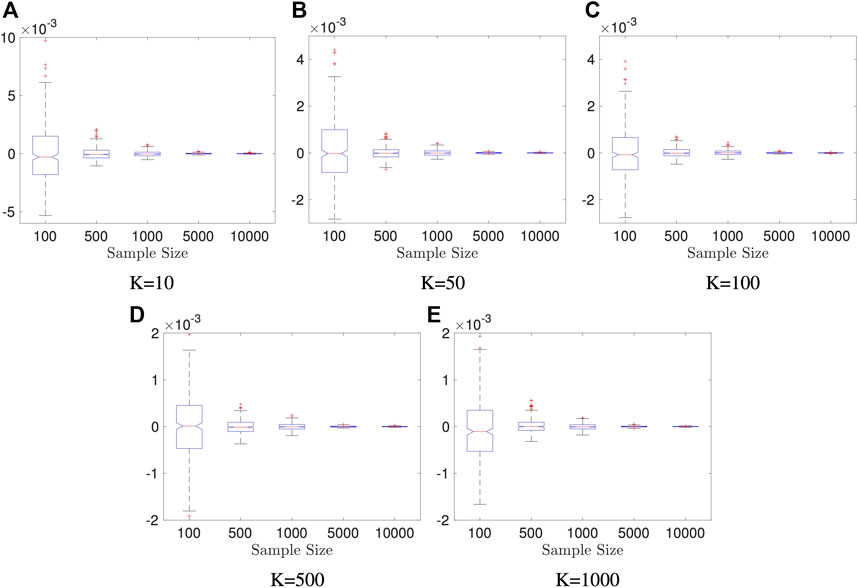
FIGURE 1. Boxplots of estimators in Example 5.1: dimension of X and Y is fixed to be p = q = 10; the result is based on 400 repeated experiments. In each subplot, y-axis represents the value of distance covariance estimators.

Example 5.2 We generate random vectors $X\in {\mathbb{R}}^{10}$ and $Y\in {\mathbb{R}}^{10}$ Each entry X_i follows Unif(0, 1), independently. Let Y_i denote the i-th entry of Y. We let $Y_1=X_1^2$ and $Y_2=X_2^2$ The rest entry of Y, $Y_i=Z_i^2$, i = 3, …, 10, where Z_i follows Unif(0, 1), independently.See Figure 2 for the boxplots of the outcomes of Example 5.2. In each subfigure, we fix the number of the Monte Carlo iterations K and let the number of observations n grow. This example shows that if K is fixed, the variation of the estimator remains regardless of the sample size n. In the dependent cases, the number of the Monte Carlo iterations K plays a more important role in estimator convergence than sample size n.The outcomes of Example 5.1 and 5.2 confirm the theoretical results that the proposed estimator converges to 0 as sample size n grows in the independent case, and converges to some nonzero number as the number of the Monte Carlo iterations K grows in the dependent case.In the following two examples, we fix the sample size n = 2000 as we noticed that our method is more efficient than the direct method when n is large. We fix the number of the Monte Carlo iterations K = 50 and relax the restriction on the data dimensions to allow p ≠ q and let p, q vary in (10, 50, 100, 500, 1000). We continue with an independent case as follows.

FIGURE 2

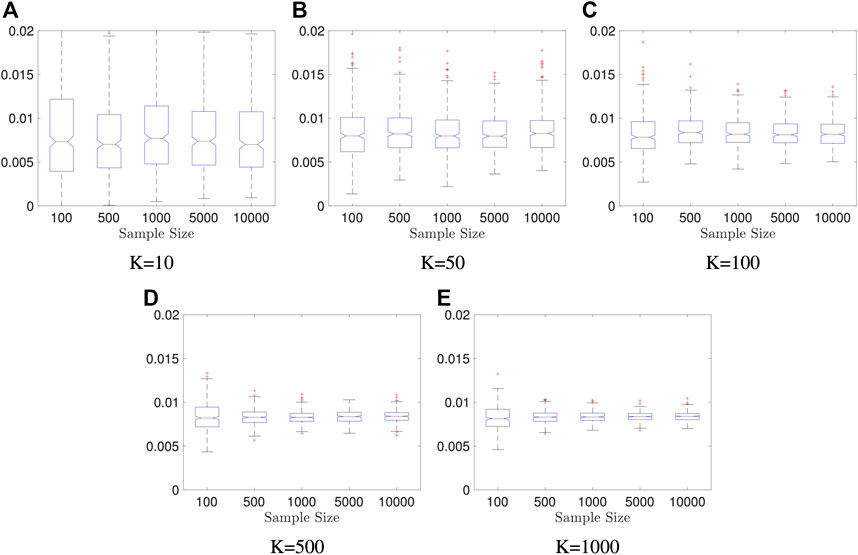
FIGURE 2. Boxplots of our estimators in Example 5.2: dimension of X and Y is fixed to be p = q = 10; the result is based on 400 repeated experiments. In each subplot, y-axis represents the value of distance covariance estimators.

Example 5.3 We generate random vectors $X\in {\mathbb{R}}^p$ and $Y\in {\mathbb{R}}^q$. Each entry of X follows Unif(0, 1), independently. Each entry $Y_i=Z_i^2$, where Z_i follows Unif(0, 1), independently.See Figure 3 for the boxplots of the outcomes of Example 5.3. In each subfigure, we fix the dimension of X and let the dimension of Y grow. It is worth noting that the scale of each subfigure could be different to display the entire boxplots. It shows that the proposed estimator converges fairly fast in independent cases regardless of the dimension of the data.The following presents a dependent case. In this case, only a small number of entries in X and Y are dependent, which means that the dependency structure between X and Y is low-dimensional though X or Y could be of high dimensions.

FIGURE 3

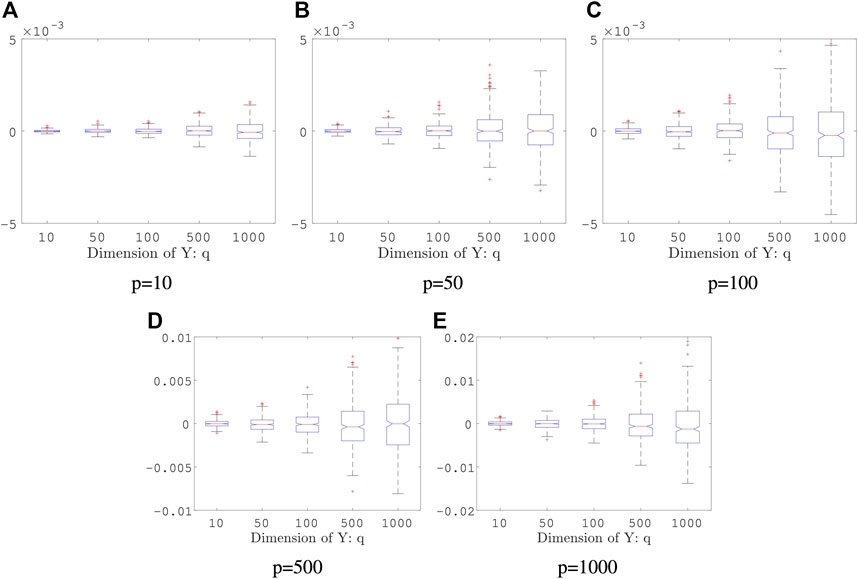
FIGURE 3. Boxplot of Estimators in Example 5.3: both sample size and the number of Monte Carlo iterations is fixed, n = 2000, K = 50; the result is based on 400 repeated experiments. In each subplot, y-axis represents the value of distance covariance estimators.

Example 5.4 We generate random vectors $X\in {\mathbb{R}}^p$ and $Y\in {\mathbb{R}}^q$. Each entry of X follows Unif(0, 1), independently. We let the first 5 entries of Y to be the square of the first 5 entries of X and let the rest entries of Y to be the square of some independent Unif(0, 1) random variables. Specifically, we let $Y_i=X_i^2,i=1,\dots ,5$, and, $Y_i=Z_i^2,i=6,\dots ,q$, where Z_i’s are drawn independently from Unif(0, 1).See Figure 4 for the boxplots of the outcomes of Example 5.4. In each subfigure, we fix the dimension of X and let the dimension of Y grow. The test power of the proposed test against data dimensions can be seen in Table 1. It is worth noting that when the sample size is fixed, the test power of our method decays as the dimension of X and Y increase. We use the Direct Distance Covariance (DDC) defined in Eq. 2.5 on the same data. As a contrast, the test power of DDC is 1.000 even p = q = 1000. This example raises a limitation of random projection: it may fail to detect the low dimensional dependency in high dimensional data. A possible remedy for this issue is performing dimension reduction before applying the proposed method. We do not research further along this direction since it is beyond the scope of this paper.

FIGURE 4

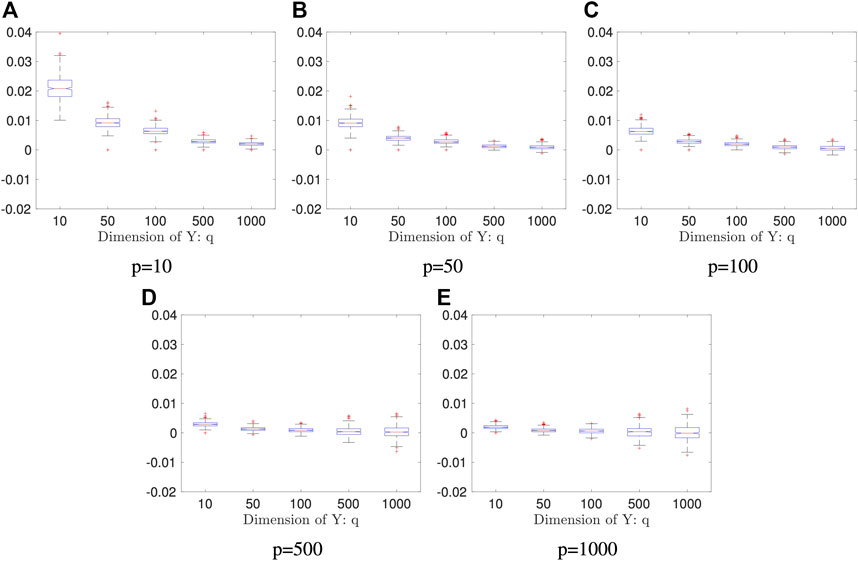
FIGURE 4. Boxplots of the proposed estimators in Example 5.4: both sample size and the number of the Monte Carlo iterations are fixed: n = 2000 and K = 50; the result is based on 400 repeated experiments. In each subplot, y-axis represents the value of distance covariance estimators.

TABLE 1

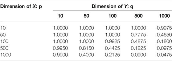
TABLE 1. Test Power in Example 5.4: this result is based 400 repeated experiments; the significance level is 0.05.

5.2 Comparison With Direct Method

In this section, we would like to illustrate the computational and space efficiency of the proposed method (RPDC). RPDC is much faster than the direct method (DDC, Eq. 2.5) when the sample size is large. It is worth noting that DDC is infeasible when the sample size is too large as its space complexity is O(n²). See Table 2 for a comparison of computing time (unit: second) against the sample size n. This experiment is run on a laptop (MacBook Pro Retina, 13-inch, Early 2015, 2.7 GHz Intel Core i5, 8 GB 1867 MHz DDR3) with MATLAB R2016b (9.1.0.441655).

TABLE 2

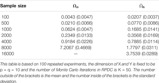
TABLE 2. Speed Comparison: Direct Distance Covariance vs. Randomly Projected Distance Covariance.

5.3 Comparison With Other Independence Tests

In this part, we compare the statistical test power of the proposed test (RPDC) with Hilbert-Schmidt Independence Criterion (HSIC) [4] as HSIC is gaining attention in machine learning and statistics communities. In our experiments, a Gaussian kernel with standard deviation σ = 1 is used for HSIC. We also compare with Randomized Dependence Coefficient (RDC) [16], which utilizes the technique of random projection as we do. Two classical tests for multivariate independence, which are described below, are included in the comparison as well as Direct Distance Covariance (DDC) defined in Eq. 2.5.

• Wilks Lambda (WL): the likelihood ratio test of hypotheses Σ₁₂ = 0 with μ unknown is based on

$\frac{\det (S)}{\det (S_{11})\det (S_{22})}=\frac{\det (S_{22}-S_{21}{S}_{11}^{-1}{S}_{12})}{\det (S_{22})},$

where det(⋅) is the determinant, S, S₁₁ and S₂₂ denote the sample covariances of (X, Y), X and Y, respectively, and S₁₂ is the sample covariance $\widehat{\text{Cov}}(X,Y)$. Under multivariate normality, the test statistic

$W=-n\log \det (I-S_{22}^{-1}{S}_{21}{S}_{11}^{-1}{S}_{12})$

has the Wilks Lambda distribution Λ(q, n − 1 − p, p), see [17].

• Puri-Sen (PS) statistics: [18], Chapter 8, proposed similar tests based on more general sample dispersion matrices T. In that test S, S₁₁, S₁₂ and S₂₂ are replaced by T, T₁₁, T₁₂ and T₂₂, where T could be a matrix of Spearman’s rank correlation statistics. Then, the test statistic becomes

$W=-n\log \det (I-T_{22}^{-1}{T}_{21}{T}_{11}^{-1}{T}_{12})$

The critical values of the Wilks Lambda (WL) and Puri-Sen (PS) statistics are given by Bartlett’s approximation ([19], Section 5.3.2b): if n is large and p, q > 2, then

$-\left(n-\frac{1}{2}(p+q+3)\right)\log \det (I-S_{22}^{-1}{S}_{21}{S}_{11}^{-1}{S}_{12})$

has an approximation χ²(pq) distribution.

The reference distributions of RDC and HSIC are approximated by 200 permutations. And the reference distributions of DDC and RPDC are approximated by Gamma Distribution. The significance level is set to be α_s = 0.05 and each experiment is repeated for N = 400 times to get reliable type-I error/test power.

We start with an example that (X, Y) is multivariate normal. In this case, WL and PS are expected to be optimal as the assumptions of these two classical tests are satisfied. Surprisingly, DDC has comparable performance with the aforementioned two methods. RPDC can achieve satisfactory performance when the sample size is reasonably large.

Example 5.5 We set the dimension of the data to be p = q = 10. We generate random vectors $X\in {\mathbb{R}}^{10}$ and $Y\in {\mathbb{R}}^{10}$ from the standard multivariate normal distribution $\mathcal{N}(0,{\mathbf{I}}_{10})$. The joint distribution of (X, Y) is also normal and we have Cor(X_i, Y_i) = ρ, i = 1, …, 10, and the rest correlation are all 0. We set the value of ρ to be 0 and 0.1 to represent independent and correlated scenarios, respectively. The sample size n is set to be from 100 to 1500 with an increment of 100.Figure 5 plots the type-I error in subfigure (a) and test power in subfigure (b) against sample size. In the independence case (ρ = 0.0), the type-I error of each test is always around the significance level α_s = 0.05, which implies the Gamma approximation works well for asymptotic distributions. In the dependent case (ρ = 0.1), the overall performance of RPDC is close to HSIC and RPDC outperforms when the sample size is smaller and underperforms when the sample size is larger. Unfortunately, RDC’s test power is insignificant.Next, we compare those methods when (X, Y) is no longer multivariate normal and the dependency between X and Y is non-linear. We even add a noise term to compare their performance in both low and high noise-to-signal ratio scenarios. In this case, DDC and RPDC are much better than WL, PS, and RDC. The performance of HSIC is close to DDC and RPDC when the noise is low but much worse than those two when the noise is high.

FIGURE 5

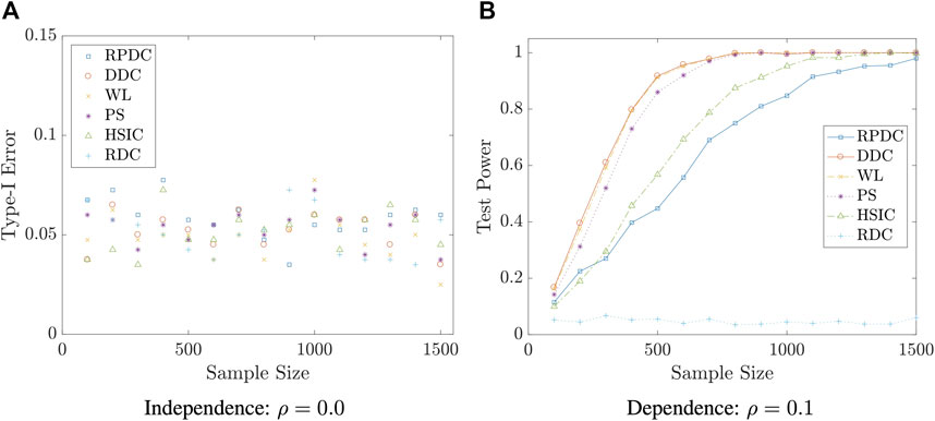
FIGURE 5. Type-I Error/Test Power vs. Sample Size n in Example 5.5: the result is based on 400 repeated experiments.

Example 5.6 We set the dimension of data to be p = q = 10. We generate random vector $X\in {\mathbb{R}}^{10}$ from the standard multivariate normal distribution $\mathcal{N}(0,{\mathbf{I}}_{10})$. Let the i-th entry of Y be $Y_i=\log (X_i^2)+{ϵ}_i,i=1,\dots ,q$, where ϵ_i’s are independent random errors, ${ϵ}_i\sim \mathcal{N}(0,{\sigma }^2)$. We set the value of σ to be 1 and 3 to represent low and high noise ratios, respectively. In the σ = 1 case, the sample size n is from 100 to 1000 with an increment 20; and in the σ = 3 case, the sample size n is from 100 to 4000 with an increment 100.Figure 6 plots the test power of each test against sample size. In both low and high noise cases, none of WL, PS, and RDC has any test power. In the low noise case, all of RPDC, DDC, and HSIC have satisfactory test power (> 0.9) when the sample size is greater than 300. In the high noise case, RPDC and DDC could achieve more than 0.8 in test power once the sample size is greater than 500 while the test power of HSIC reaches 0.8 when the sample size is more than 2000.In the following example, we generate the data similarly with Example 5.6 but the difference is that the dependency is changing over time. Specifically, X and Y are independent at the beginning but they become dependent after some time point. Since all those tests are invariant with the order of the observations, this experiment simply means that only a proportion of observations are dependent while the rest are not.

FIGURE 6

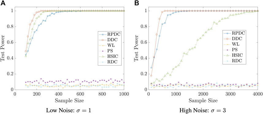
FIGURE 6. Test Power vs. Sample Size n in Example 5.6: significance level is α_s = 0.05; the result is based on N = 400 repeated experiments.

Example 5.7 We set the dimension of data to be p = q = 10. We generate random vector $X_t\in {\mathbb{R}}^{10},t=1,\dots ,n$, from the standard multivariate normal distribution $\mathcal{N}(0,{\mathbf{I}}_{10})$. Let the i-th entry of Y_t be $Y_{t,i}=\log (Z_{t,i}^2)+{ϵ}_{t,i},t=1,\dots ,T$ and $Y_{t,i}=\log (X_{t,i}^2)+{ϵ}_{t,i},t=T+1,\dots ,n$, where $Z_{t}i.i.d.\sim \mathcal{N}(0,{\mathbf{I}}_{10})$ and ϵ_t,i’s are independent random errors, ${ϵ}_{t,i}\sim \mathcal{N}(\mathrm{0,1})$. We set the value of T to be 0.5n and 0.8n to represent early and late dependency transition, respectively. In the early change case, the sample size n is from 500 to 2000 with an increment 100; and in the late change case, the sample size n is from 500 to 4000 with an increment 100.Figure 7 plots the test power of each test against sample size. In both early and late change cases, none of WL, PS, and RDC has any test power. In the early change case, all of RPDC, DDC, and HSIC have satisfactory test power (> 0.9) when the sample size is greater than 1500. In the late change case, DDC and HSIC could achieve more than 0.8 in test power once sample size reaches 4000 while the test power of RPDC is only 0.6 when the sample size is 4000. As expected, the performance of DDC is better than RPDC in both cases and the performance of HSIC is between DDC and RPDC.

FIGURE 7

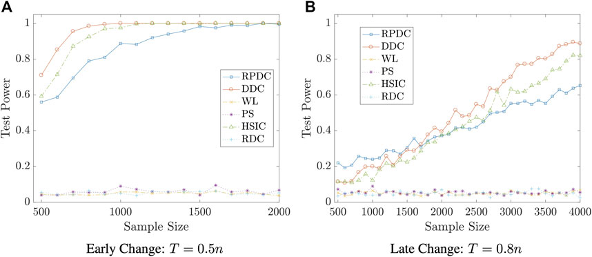
FIGURE 7. Test Power vs. Sample Size n in Example 5.7: significance level is α_s = 0.05; the result is based on N = 400 repeated experiments.

Remark 5.8 The examples in this subsection show that though RPDC underperforms DDC when the sample size is relatively small, RPDC could achieve the same test power with DDC when the sample size is sufficiently large. Thus, when the sample size is large enough, RPDC is superior to DDC because of its computational efficiency in both time and space.

6 Discussions

6.1 A Discussion on the Computational Efficiency

We compare the computational efficiency of the proposed method (RPDC) and the direct method (DDC) in Section 5.2. We will discuss this issue here.

As $X\in {\mathbb{R}}^p$ and $Y\in {\mathbb{R}}^q$ are multivariate random variables, the effect of p and q on computing time could be significant when p and q are not negligible compared to sample size n. Now, we analyze the computational efficiency of DDC and RPDC by taking p and q into consideration. The computational complexity of DDC becomes O(n²(p + q)) and that of RPDC becomes O(nK( log  n + p + q)). Let us denote the total number of operations in DDC by O₁ and that in RPDC by O₂. Then, there exist constants L₁ and L₂ such that

$O_1\approx L_1{n}^2(p+q)\text{,\hspace{0.17em}and\hspace{0.17em}}{O}_2\approx L_{2}nK(\log n+p+q).$

There is no doubt that O₂ will eventually be much less than O₁ as sample size n grows. Due to the complexity of the fast algorithm, we expect L₂ > L₁, which means the computing time of RPDC is even larger than DDC when the sample size is relatively small. Then, we need to study an interesting problem: what is the break-even point in terms of sample size n when RPDC and DDC have the same computing time?

Let n₀ = n₀(p + q, K) denote the break-even point, which is a function of p + q and number of Monte Carlo iterations K. For simplicity, we fix K = 50 since 50 iterations could achieve satisfactory test power as we showed in Example 5.4. Then, n₀ becomes a function solely depending on p + q. Since it is hard to derive the close form of n₀, we derive it numerically instead. For fixed p + q, we let the sample size vary and record the difference between the running time of the two methods. Then, we fit the difference of running time against sample size with a smoothing spline. The root of this spline is the numerical value of n₀ at p + q.

We plot the n₀ against p + q in Figure 8. As the figure shows, the break-even sample size decreases as the data dimension increases, which implies that our proposed method is more advantageous than the direct method when random variables are of high dimension. However, as shown in Example 5.4, the random projection-based method does not perform well when high dimensional data have a low dimensional dependency structure. We should be cautious to use the proposed method when the dimension is high.

FIGURE 8

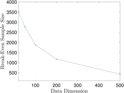
FIGURE 8. Break-Even Sample Size n₀ against Data Dimension p + q. This figure is based on 100 repeated experiments.

6.2 Connections With Existing Literature

It turns out that distance-based methods are not the only choices in independence tests. See [20] and the references therein to see alternatives.

Our proposed method utilizes random projections, which bears a similarity with the randomized feature mapping strategy [21] that was developed in the machine learning community. Such an approach has been proven to be effective in kernel-related methods [22–26]. However, a closer examination will reveal the following difference: most of the aforementioned work is rooted in the Bochner’s theorem [27] from harmonic analysis, which states that a continuous kernel in the Euclidean space is positive definite if and only if the kernel function is the Fourier transform of a non-negative measure. In this paper, we will deal with the distance function which is not a positive definite kernel. We will manage to derive a counterpart to the randomized feature mapping, which was the influential idea that has been used in [21].

Random projections have been used in [28] to develop a powerful two-sample test in high dimensions. They derived an asymptotic power function for their proposed test, and then provide sufficient conditions for their test to achieve greater power than other state-of-the-art tests. They then used the receiver operating characteristic (ROC) curves (that are generated from simulated data) to evaluate its performance against competing tests. The derivation of the asymptotic relative efficiency (ARE) is of its own interests. Despite the usage of random projection, the details of their methodology are very different from the one that is studied in the present paper.

Several distribution-free tests that are based on sample space partitions were suggested in [29] for univariate random variables. They proved that all suggested tests are consistent and showed the connection between their tests and the mutual information (MI). Most importantly, they derived fast (polynomial-time) algorithms, which are essential for large sample size, since the computational complexity of the naive algorithm is exponential in sample size. Efficient implementations of all statistics and tests described in the aforementioned paper are available in the R package HHG, which can be freely downloaded from the Comprehensive R Archive Network, http://cran.r-project.org/. Null tables can be downloaded from the first author’s website.

Distance-based independence/dependence measurements sometimes have been utilized in performing a greedy feature selection, often via dependence maximization [8,30,31], and it has been effective on some real-world datasets. This paper simply mentions such a potential research line, without pursuing it.

Paper [32] derives an efficient approach to compute for the conditional distance correlations. We noted that there are strong resemblances between the distance covariances and its conditional version. The search for a potential extension of the work in this paper to conditional distance correlation can be a meaningful future topic of research.

Paper [33] provides some important insights into the power of distance covariance for multivariate data. In particular, they discover that distance-based independence tests have limiting power under some less common circumstances. As a remedy, they propose tests based on an aggregation of marginal sample distance and extend their approach to those based on Hilbert-Schmidt covariance and marginal distance/Hilbert-Schmidt covariance. It could be another interesting research direction but beyond the scope of this paper.

7 Conclusion

A significant contribution of this paper is we demonstrated that the multivariate variables in the independence tests need not imply the higher-order computational desideratum of the distance-based methods.

Distance-based methods are important in statistics, particularly in the test of independence. When the random variables are univariate, efficient numerical algorithms exist. It is an open question when the random variables are multivariate. This paper studies the random projection approach to tackle the above problem. It first turns the multivariate calculation problem into univariate calculation one via a random projection. Then they study how the average of those statistics out of the projected (therefore univariate) samples can approximate the distance-based statistics that were intended to use. Theoretical analysis was carried out, which shows that the loss of asymptotic efficiency (in the form of the asymptotic variance of the test statistics) is likely insignificant. The new method can be numerically much more efficient, when the sample size is large, which is well-expected under this information (or big-date) era. Simulation studies validate the theoretical statements. The theoretical analysis takes advantage of some newly available results, such as the equivalence of the distance-based methods with the reproducible kernel Hilbert spaces [12]. The numerical methods utilize a recently appeared algorithm in [8].

Data Availability Statement

The original contributions presented in the study are included in the article/Supplementary Material, further inquiries can be directed to the corresponding author.

Author Contributions

All authors listed have made a substantial, direct, and intellectual contribution to the work and approved it for publication.

Conflict of Interest

The authors declare that the research was conducted in the absence of any commercial or financial relationships that could be construed as a potential conflict of interest.

Publisher’s Note

All claims expressed in this article are solely those of the authors and do not necessarily represent those of their affiliated organizations, or those of the publisher, the editors and the reviewers. Any product that may be evaluated in this article, or claim that may be made by its manufacturer, is not guaranteed or endorsed by the publisher.

Acknowledgments

This material was based upon work partially supported by the National Science Foundation under Grant DMS-1127914 to the Statistical and Applied Mathematical Sciences Institute. Any opinions, findings, and conclusions, or recommendations expressed in this material are those of the author(s) and do not necessarily reflect the views of the National Science Foundation. This work has also been partially supported by NSF grant DMS-1613152.

Supplementary Material

The Supplementary Material for this article can be found online at: https://www.frontiersin.org/articles/10.3389/fams.2021.779841/full#supplementary-material

References

1. David, N, Yakir, A, Hilary, K, Sharon, R, Peter, J, Eric, S, et al. Detecting Novel Associations in Large Data Sets. Science (2011) 334(6062):1518–24.

PubMed Abstract | Google Scholar

2. Schweizer, B, and Wolff, EF. On Nonparametric Measures of Dependence for Random Variables. Ann Stat (1981) 879–85. doi:10.1214/aos/1176345528

CrossRef Full Text | Google Scholar

3. Siburg, KF, and Stoimenov, PA. A Measure of Mutual Complete Dependence. Metrika (2010) 71(2):239–51. doi:10.1007/s00184-008-0229-9

CrossRef Full Text | Google Scholar

4. Gretton, A, Bousquet, O, Smola, A, and Schölkopf, B. Measuring Statistical Dependence with hilbert-schmidt Norms. International Conference on Algorithmic Learning Theory. Springer (2005). p. 63–77. doi:10.1007/11564089_7

CrossRef Full Text | Google Scholar

5. Székely, GJ, and Rizzo, ML. Brownian Distance Covariance. Ann Appl Stat (2009) 3(4):1236–65. doi:10.1214/09-aoas312

CrossRef Full Text | Google Scholar

6. GáborSzékely, J, MariaRizzo, L, and Bakirov, NK. Measuring and Testing Dependence by Correlation of Distances. Ann Stat (2007) 35(6):2769–94. doi:10.1214/009053607000000505

CrossRef Full Text | Google Scholar

7. Matthew, R, and Nicolae, DL. On Quantifying Dependence: a Framework for Developing Interpretable Measures. Stat Sci (2013) 28(1):116–30.

Google Scholar

8. Huo, X, and Székely, GJ. Fast Computing for Distance Covariance. Technometrics (2016) 58(4):435–47. doi:10.1080/00401706.2015.1054435

CrossRef Full Text | Google Scholar

9. Taskinen, S, Oja, H, and Randles, RH. Multivariate Nonparametric Tests of independence. J Am Stat Assoc (2005) 100(471):916–25. doi:10.1198/016214505000000097

CrossRef Full Text | Google Scholar

10. Lyons, R. Distance Covariance in Metric Spaces. Ann Probab (2013) 41(5):3284–305. doi:10.1214/12-aop803

CrossRef Full Text | Google Scholar

11. Hoeffding, W. Probability Inequalities for Sums of Bounded Random Variables. J Am Stat Assoc (1963) 58(301):13–30. doi:10.1080/01621459.1963.10500830

CrossRef Full Text | Google Scholar

12. Sejdinovic, D, Sriperumbudur, B, Gretton, A, and Fukumizu, K. Equivalence of Distance-Based and RKHS-Based Statistics in Hypothesis Testing. Ann Stat (2013) 41(5):2263–91. doi:10.1214/13-aos1140

CrossRef Full Text | Google Scholar

13. Serfling, RJ. Approximation Theorems of Mathematical Statistics (Wiley Series in Probability and Statistics). Wiley-Interscience (1980).

Google Scholar

14. George, EP, Some Theorems on Quadratic Forms Applied in the Study of Analysis of Variance Problems, I. Effect of Inequality of Variance in the One-Way Classification. Ann Math Stat (1954) 25(2):290–302.

Google Scholar

15. DeanBodenham, A, and Adams, NM. A Comparison of Efficient Approximations for a Weighted Sum of Chi-Squared Random Variables. Stat Comput pages (2014) 1–12.

Google Scholar

16. Lopez-Paz, D, Hennig, P, and Schölkopf, B. The Randomized Dependence Coefficient. In Advances in Neural Information Processing Systems, 1–9. 2013.

Google Scholar

17. Wilks, SS. On the Independence of K Sets of Normally Distributed Statistical Variables. Econometrica (1935) 3:309–26. doi:10.2307/1905324

CrossRef Full Text | Google Scholar

18. Puri, ML, and Sen, PK. Nonparametric Methods in Multivariate Analysis. Wiley Series in Probability and Mathematical Statistics. Probability and mathematical statistics. Wiley (1971).

Google Scholar

19. Mardia, KV, Bibby, JM, and Kent, JT. Multivariate Analysis. New York, NY: Probability and Mathematical Statistics. Acad. Press (1982).

Google Scholar

20. Lee, K-Y, Li, B, and Zhao, H. Variable Selection via Additive Conditional independence. J R Stat Soc Ser B (Statistical Methodology) (2016) 78(Part 5):1037–55. doi:10.1111/rssb.12150

CrossRef Full Text | Google Scholar

21. Rahimi, A, and Recht, B. Random Features for Large-Scale Kernel Machines. In Advances in Neural Information Processing Systems, 1177–84. 2007.

Google Scholar

22. Achlioptas, D, McSherry, F, and Schölkopf, B. Sampling Techniques for Kernel Methods. In Annual Advances In Neural Information Processing Systems 14: Proceedings Of The 2001 Conference (2001).

Google Scholar

23. Avrim, B. Random Projection, Margins, Kernels, and Feature-Selection. In Subspace, Latent Structure and Feature Selection, 52–68. Springer, 2006.

Google Scholar

24. Cai, T, Fan, J, and Jiang, T. Distributions of Angles in Random Packing on Spheres. J Mach Learn Res (2013) 14(1):1837–64.

PubMed Abstract | Google Scholar

25. Drineas, P, and Mahoney, MW. On the Nyström Method for Approximating a Gram Matrix for Improved Kernel-Based Learning. J Machine Learn Res (2005) 6(Dec):2153–75.

Google Scholar

26. Frieze, A, Kannan, R, and Vempala, S. Fast Monte-Carlo Algorithms for Finding Low-Rank Approximations. J Acm (2004) 51(6):1025–41. doi:10.1145/1039488.1039494

CrossRef Full Text | Google Scholar

27. Rudin, W. Fourier Analysis on Groups. John Wiley & Sons (1990).

Google Scholar

28. Miles, L, Laurent, J, and Wainwright, J. A More Powerful Two-Sample Test in High Dimensions Using Random Projection. In Advances in Neural Information Processing Systems, 1206–14. 2011.

Google Scholar

29. Heller, R, Heller, Y, Kaufman, S, Brill, B, and Gorfine, M. Consistent Distribution-free K-Sample and independence Tests for Univariate Random Variables. J Machine Learn Res (2016) 17(29):1–54.

Google Scholar

30. Li, R, Zhong, W, and Zhu, L. Feature Screening via Distance Correlation Learning. J Am Stat Assoc (2012) 107(499):1129–39. doi:10.1080/01621459.2012.695654

PubMed Abstract | CrossRef Full Text | Google Scholar

31. Zhu, L-P, Li, L, Li, R, and Zhu, L-X. Model-free Feature Screening for Ultrahigh-Dimensional Data. J Am Stat Assoc (2012).

Google Scholar

32. Wang, X, Pan, W, Hu, W, Tian, Y, and Zhang, H. Conditional Distance Correlation. J Am Stat Assoc (2015) 110(512):1726–34. doi:10.1080/01621459.2014.993081

CrossRef Full Text | Google Scholar

33. Zhu, C, Zhang, X, Yao, S, and Shao, X Distance-based and Rkhs-Based Dependence Metrics in High Dimension. Ann Stat (2020) 48(6):3366–94. doi:10.1214/19-aos1934

CrossRef Full Text | Google Scholar