A New Two-Parameter Estimator for Beta Regression Model: Method, Simulation, and Application

Introduction

The beta regression model has been common in many areas, primarily economic and medical research, such as income share, unemployment rates in certain nations, the Gini index for each region, graduation rates in major universities, or the percentage of body fat in medical subjects. Beta regression model, such as any regression model in the context of generalized linear models (GLMs) is used to examine the effect of certain explanatory variables on a non-normal response variable. However, in the case of beta regression, the response component is restricted to an interval (0, 1), such as proportions, percentages, and fractions.

Multicollinearity is a popular issue in econometric modeling. It indicates that there is a strong association between the explanatory variables. It is well-established that the covariance matrix of the maximum likelihood (ML) estimator is ill-conditioned in the case of severing multicollinearity. One of the negative consequences of this issue is that the variance of the regression coefficients gets inflated. As a consequence, the significance and the magnitude of the coefficients are affected. Many of the conventional approaches used to address this issue include: gathering additional data, re-specifying the model, or removing the correlated variable/s.

During the last years, shrinkage methods have become a commonly recognized and more effective methodology for solving the impact of the multicollinearity problem in several regression models. To solve this problem, Hoerl and Kennard [1, 2] proposed the ridge estimator. The concept of the ridge estimator is to add a small definite amount (k) to the diagonal entries of the covariance matrix to increase the conditioning of this matrix, reduce the mean squared error (MSE), and achieve consistent coefficients. For a review of the ridge estimator in both linear and GLMs, e.g., as shown in References Rady et al. [3], Abonazel and Taha [4], Qasim et al. [5], Alobaidi et al. [6], and Sami et al. [7].

One of the drawbacks of the ridge estimator is that estimated parameters are non-linear functions of the ridge parameter and the small k selected might not be high enough to solve multicollinearity. As a solution to this problem, Liu [8] developed the Liu estimator which is a linear function of the shrinkage parameter. The Liu estimator is a combination of the ridge estimator and the Stein estimator suggested by Stein [9]. For a review of the Liu estimator in both linear and GLMs, e.g., as shown in References. Liu [8], Karlsson et al. [10], Qasim et al. [11], and Naveed et al. [12]. Furthermore, Liu [13] proved the supremacy of the Liu-type estimator over the ridge and Liu estimators. Details about Liu-type estimator, properties, and applications in regression models are shown in References Liu [14], Özkale and Kaciranlar [15], Li and Yang [16], Kurnaz and Akay [17], Sahriman and Koerniawan [18], and Algamal and Abonazel [19]. As a good alternative for the Liu-type estimator, Özkale and Kaciranlar [15] proposed the two-parameter estimator, and they proved that the two-parameter estimator utilizes the power of both the ridge estimator and the Liu estimator. Extensions of two-parameter estimator in GLMs include Huang and Yang [20], Algamal [21], Asar and Genç [22], Rady et al. [23, 24], Çetinkaya and Kaçiranlar [25], Abonazel and Farghali [26], Akram et al. [27], and Lukman et al. [28].

The rest of the article is arranged as follows: Section Methodology presents an introduction about the beta regression model, its estimation using the ML method, and the proposed two-parameter estimator; Section Choosing the Shrinkage Parameters provides suggested shrinkage parameters for our estimator; Sections Simulation Study and Real Data Applications provide a numerical evaluation using both Monte Carlo simulation and two empirical data applications, respectively; and Section Conclusion offers some concluding remarks.

Methodology

Beta Regression Model

Practitioners usually use linear regression modeling to investigate the relationship and effect of some selected explanatory variables on the normal response variable. However, this is not suitable for circumstances where the response variable is constrained to the interval (0, 1) because it may give fitted values for the variable of concern that surpass its lower and upper limits. Therefore, inference based on the normality assumption can be deceptive. The beta regression model was first developed by Ferrari and Cribari-Neto [29] by connecting the mean function of its response variable to a set of linear predictors via a monotone differentiable function called the link function. This model contains a precision parameter, the inverse of which is called a dispersion scale. In the basic type of a beta regression model, the precision parameter is believed to be constant through observations. Nevertheless, the precision parameter might not be constant through findings such as those of Smithson and Verkuilen [30] and Cribari-Neto and Zeileis [31].

Let y is a continuous random variable that follows a beta distribution with the following probability density function:

$\begin{array}{l}\text{f}(y;\mu ,\varphi )=\frac{\Gamma (\varphi )}{\Gamma (\mu \varphi )\Gamma ((1-\mu )\varphi )}y{}^{(\mu \varphi )-1}{(1-y)}^{(\varphi -\mu \varphi -1)};\\ 0<y<1;0<\mu <1;\varphi >0,& (1)\end{array}$

where Γ(·) is the gamma function and ϕ is the precision parameter [32]:

$\begin{array}{l}\varphi =\frac{1-{\sigma }^2}{{\sigma }^2}.\end{array}$

The mean and variance of the beta probability distribution are: E(y) = μ, var(y) = μ(1 − μ)σ². Using the logit link function, the model allows μ_i, depending on covariates as follows:

$\begin{array}{ll}\text{g}({\mu }_i)=\text{log }\left(\frac{{\mu }_i}{1-{\mu }_i}\right)={\text{x}}_i^T\beta ={\eta }_i,& (2)\end{array}$

where g(·) be a monotonic differentiable link function used to relate the systematic component with the random component, $\beta ={\left({\beta }_1,\dots ,{\beta }_p\right)}^T$ is a p × 1 vector of unknown parameters, ${\mathrm{\text{x}}}_i={\left(\begin{array}{c}{x}_{i1},\dots ,x_{ip}\end{array}\right)}^T$ is the vector of p regressors, and η_i is a linear predictor.

Estimation of the beta regression parameters is done by using the ML method [33]. The log-likelihood function of the beta regression model is given by:

$\begin{array}{l}{L}\left({\mu }_i,\varphi ;y_i\right)={\displaystyle {\sum }_{i=1}^n\{\text{log}\Gamma (\varphi )-\text{log}\Gamma ({\mu }_i(\varphi ))}\\ -\text{log}\Gamma ((1-{\mu }_i)(\varphi ))+({\mu }_i(\varphi )-1)\text{log}(y_i)\\ +((1-\mu )(\varphi )-1)\text{log}(1-y_i)\}& (3)\end{array}$

By differentiating the log-likelihood function in Eq. (3) with respect to β, gives us the score function for β:

$\begin{array}{ll}S(\beta )=\varphi X^{T}A(y^{*}-{\mu }^{*}),& (4)\end{array}$

where $A=\mathrm{\text{diag}}\left(\frac{1}{{\mathrm{\text{g}}}^{{}^{\prime }}({\mu }_1)},\dots ,\frac{1}{{\mathrm{\text{g}}}^{\prime }({\mu }_n)}\right)$, $y^{*}={\left(y_1^{*},\dots ,y_n^{*}\right)}^T$, ${\mu }^{*}={\left({\mu }_1^{*},\dots ,{\mu }_n^{*}\right)}^T$, $y_i^{*}=log\left(\frac{y_i}{1-y_i}\right)$, and ${\mu }_i^{*}=\psi ({\mu }_i\varphi )-\psi ((1-{\mu }_i)\varphi )$, such that ψ(·) denoting the digamma function, and g′(·) is the first derivative of g(·). The iterative reweighted least-squares (IWLS) algorithm or Fisher's scoring algorithm was used for estimating β [34, 35]. The form of this algorithm can be written as:

$\begin{array}{l}{\beta }^{(r+1)}={\beta }^{(r)}+{\left(I_{\beta \beta }^{(r)}\right)}^{-1}{S}_{\beta }^{(r)}(\beta ),\end{array}$

where $S_{\beta }^{(r)}$ is the score function defined in Eq. (4), and ${\text{I}}_{\beta \beta }^{(r)}$ is the information matrix for β , as shown in References Espinheira et al. [35] for more details. The initial value of β can be obtained by the least-squares estimation, while the initial value for each precision parameter is:

$\begin{array}{ll}{\widehat{\varphi }}_i=\frac{{\widehat{\mu }}_i\left(1-{\widehat{\mu }}_i\right)}{{\widehat{\sigma }}_i^2},& (5)\end{array}$

where $\widehat{\mu }$ and ${\widehat{\sigma }}_i^2$ values are obtained from linear regression. Given r = 0, 1, 2, … is the number of iterations that are performed, convergence occurs when the difference between successive estimates becomes smaller than a given small constant. At the final step, the ML estimator of β is obtained as:

$\begin{array}{ll}{\widehat{\beta }}_{\text{BML}}={\left(X^TŴX\right)}^{-1}{X}^TŴẑ,& (6)\end{array}$

where X is an n×p matrix of regressors, $ẑ=\widehat{\eta }+{Ŵ}^{-1}Â\left(y^{*}-{\mu }^{*}\right)$, and Ŵ = diag (ŵ₁, …, ŵ_n);

$\begin{array}{l}{\widehat{w}}_i=\frac{\left(1-{\widehat{\sigma }}^2\right)}{{\widehat{\sigma }}^2}\{{\psi }^{\prime }\left(\frac{{\widehat{\mu }}_i\left(1-{\widehat{\sigma }}^2\right)}{{\widehat{\sigma }}^2}\right)\\ +{\psi }^{\prime }\left(\frac{(1-{\widehat{\mu }}_i)(1-{\widehat{\sigma }}^2)}{{\widehat{\sigma }}^2}\right)\}\frac{1}{{\left\{{\text{g}}^{\prime }\left({\widehat{\mu }}_i\right)\right\}}^2},\end{array}$

where Ŵ and  are the estimated ML matrices of W and A, respectively. The ML estimator of β is normally distributed with asymptotic mean vectors $E\left({\widehat{\beta }}_{\mathrm{\text{BR}}}\right)=\beta$ and asymptotic covariance matrix:

$\begin{array}{ll}\text{Cov}\left({\widehat{\beta }}_{\text{BML}}\right)=\frac{1}{\varphi }{\left(X^TŴX\right)}^{-1}& (7)\end{array}$

Hence, the asymptotic trace mean squared error (TMSE) of ${\widehat{\beta }}_{\mathrm{\text{BML}}}$ is

$\begin{array}{ll}\text{TMSE}\left({\widehat{\beta }}_{\text{BML}}\right)=\text{tr}\left[\frac{1}{\varphi }{(X^TŴX)}^{-1}\right]& (8)\end{array}$

Ridge and Liu Estimators

Recently, Abonazel and Taha [4] and Qasim et al. [5] introduced the ridge beta regression (RBR) estimator as follows:

$\begin{array}{ll}{\widehat{\beta }}_{\text{RBR}}={\left(X^TŴX+k\text{I}\right)}^{-1}{X}^TŴẑ;k>0& (9)\end{array}$

It can note that if k = 0, then ${\widehat{\beta }}_{\mathrm{\text{RBR}}}={\widehat{\beta }}_{\mathrm{\text{BML}}}$. The bias vector of the RBR estimator is

$\begin{array}{ll}\text{Bias}\left({\widehat{\beta }}_{\text{RBR}}\right)=-k{\left(X^TŴX+k\text{I}\right)}^{-1}\beta & (10)\end{array}$

Suppose that λ₁ ≥ … ≥ λ_p ≥ 0 are the ordered eigenvalues of X^TŴX matrix and Q is the matrix whose columns are the eigenvectors of X^TŴX matrix. Then $\Lambda =\mathrm{\text{diag}}\left({\lambda }_1,\dots ,{\lambda }_p\right)=Q^T{X}^TŴXQ$ and α = Q^Tγ. Then, the matrix mean squared error (MMSE) of the RBR estimator is:

$\begin{array}{l}\text{MMSE}\left({\widehat{\beta }}_{\text{RBR}}\right)=\text{Cov}\left({\widehat{\beta }}_{\text{RBR}}\right)+\text{Bias}\left({\widehat{\beta }}_{\text{RBR}}\right)\text{Bias}{\left({\widehat{\beta }}_{\text{RBR}}\right)}^T\\ =\frac{1}{\varphi }\left(Q{\Lambda }_k^{-1}{\Lambda \Lambda }_k^{-1}{Q}^T\right)+k^{2}Q{\Lambda }_k^{-1}\alpha {\alpha }^T{\Lambda }_k^{-1}{Q}^T,& (11)\end{array}$

where Λ_k = diag (λ₁ + k, …, λ_p + k), and the TMSE of the RBR estimator is

$\begin{array}{l}\text{TMSE}\left({\widehat{\beta }}_{\text{RBR}}\right)=\text{tr}\left(\text{MMSE}\left({\widehat{\beta }}_{\text{RBR}}\right)\right)\\ =\frac{1}{\varphi }{{\displaystyle \sum }}_{j=1}^p\frac{{\lambda }_j}{{\left({\lambda }_j+k\right)}^2}+k^2{{\displaystyle \sum }}_{j=1}^p\frac{{\alpha }_j^2}{{\left({\lambda }_j+k\right)}^2}& (12)\end{array}$

The first term in Eq. (12) is an asymptotic variance, and the second term is a square bias. Abonazel and Taha [4] and Qasim et al. [5] showed the derivation of the MSE properties of the RBR estimator.

The Liu estimator can be extended to the beta regression model, the Liu beta regression (LBR) estimator is given by Karlsson et al. [10] as:

$\begin{array}{l}{\widehat{\beta }}_{\text{LBR}}={\left(X^TŴX+\text{I}\right)}^{-1}\left(X^TŴX+d\text{I}\right){\widehat{\beta }}_{\text{BML}};\\ 0<d<1,& (13)\end{array}$

where d is the Liu parameter, the bias vector of the LBR estimator is:

$\begin{array}{ll}\text{Bias}\left({\widehat{\beta }}_{\text{LBR}}\right)={\left(X^TŴX+\text{I}\right)}^{-1}\left(d-1\right)\beta & (14)\end{array}$

The MMSE for the LBR estimator can be derived as:

$\begin{array}{l}\text{MMSE}\left({\widehat{\beta }}_{\text{LBR}}\right)=\text{Cov}\left({\widehat{\beta }}_{\text{LBR}}\right)+\text{Bias}\left({\widehat{\beta }}_{\text{LBR}}\right)\text{Bias}{\left({\widehat{\beta }}_{\text{LBR}}\right)}^T\\ =\frac{1}{\varphi }\left({Q\Lambda }_1^{-1}{\Lambda }_d{\Lambda }^{-1}{\Lambda }_d{\Lambda }_1^{-1}{Q}^T\right)\\ +{\left(d-1\right)}^2{Q\Lambda }_1^{-1}\alpha {\alpha }^T{\Lambda }_1^{-1}{Q}^T,& (15)\end{array}$

where Λ₁ = diag (λ₁ + 1, …, λ_p + 1) and Λ_d = diag (λ₁ + d, …, λ_p + d). The TMSE of the LBR estimator is:

$\begin{array}{l}\text{TMSE}\left({\widehat{\beta }}_{\text{LBR}}\right)=\text{tr}\left(\text{MMSE}\left({\widehat{\beta }}_{\text{LBR}}\right)\right)\\ =\frac{1}{\varphi }{\displaystyle \sum _{j=1}^p}\left\{\frac{{\left({\lambda }_j+d\right)}^2}{{\lambda }_j{\left({\lambda }_j+1\right)}^2}+\frac{{\left(d-1\right)}^2{\alpha }_j^2\varphi }{{\left({\lambda }_j+1\right)}^2}\right\}& (16)\end{array}$

Recently, Algamal and Abonazel [19] developed the Liu-type beta regression (LTBR) estimator:

$\begin{array}{l}{\widehat{\beta }}_{\text{LTBR}}={(X^TŴX+kI)}^{-1}(X^TŴX-dI){\widehat{\beta }}_{\text{BML}};\\ k>0,-\infty <d<\infty & (17)\end{array}$

The bias vector of the LTBR estimator is:

$\begin{array}{ll}\text{Bias}\left({\widehat{\beta }}_{LTBR}\right)=-\left(d+k\right){\left(X^TŴX+k\text{I}\right)}^{-1}\beta & (18)\end{array}$

The MMSE of the LTBR estimator is:

$\begin{array}{l}\text{MMSE}\left({\widehat{\beta }}_{\text{LTBR}}\right)=\text{Cov}\left({\widehat{\beta }}_{\text{LTBR}}\right)+\text{Bias}\left({\widehat{\beta }}_{\text{LTBR}}\right)\text{Bias}{\left({\widehat{\beta }}_{\text{LTBR}}\right)}^T\\ =\frac{1}{\varphi }\left(Q{\Lambda }_k^{-1}{\Lambda }_{-d}{\Lambda }^{-1}{\Lambda }_{-d}{\Lambda }_k^{-1}{Q}^T\right)\\ +{\left(d+k\right)}^{2}Q{\Lambda }_k^{-1}\alpha {\alpha }^T{\Lambda }_k^{-1}{Q}^T& (19)\end{array}$

where Λ_−d = diag (λ₁ − d, …, λ_p − d). Then, the MSE of the LTBR estimator is

$\begin{array}{l}\text{MSE}\left({\widehat{\beta }}_{\text{LTBR}}\right)=\text{tr}\left(\text{MMSE}\left({\widehat{\beta }}_{\text{LTBR}}\right)\right)\\ =\frac{1}{\varphi }{{\displaystyle \sum }}_{j=1}^p\left\{\frac{{\left({\lambda }_j-d\right)}^2}{{\lambda }_j{\left({\lambda }_j+k\right)}^2}+\frac{{\left(d+k\right)}^2{\alpha }_j^2\varphi }{{\left({\lambda }_j+k\right)}^2}\right\}& (20)\end{array}$

The Proposed Estimator

In this section, we extend the two-parameter estimator introduced by Özkale and Kaçiranlar [15] to the beta regression model to combat multicollinearity and obtain more stable and accurate results. The two-parameter beta regression (TPBR) estimator can be written as follows:

$\begin{array}{l}{\widehat{\beta }}_{\text{TPBR}}={(X^TŴX+kI)}^{-1}(X^TŴX+kdI){\widehat{\beta }}_{\text{BML}};\\ k>0;0<d<1& (21)\end{array}$

It is worth noting that the TPBR estimator is a general class that has some estimators as special cases. These estimators are the LBR, RBR, and beta maximum likelihood (BML) estimators, which can be given, respectively, as follows:

$\begin{array}{l}{\displaystyle \underset{k\to 1}{lim}}{\widehat{\beta }}_{\text{TPBR}}={\widehat{\beta }}_{\text{LBR}}={\left(X^TŴX+I\right)}^{-1}\left(X^TŴX+dI\right){\widehat{\beta }}_{\text{BML}},\\ {\displaystyle \underset{d\to 0}{lim}}{\widehat{\beta }}_{\text{TPBR}}={\widehat{\beta }}_{RBR}={\left(X^TŴX+kI\right)}^{-1}\left(X^TŴX\right){\widehat{\beta }}_{\text{BML}},\\ {\displaystyle \underset{k\to 0}{lim}}{\widehat{\beta }}_{\text{TPBR}}={\widehat{\beta }}_{\text{BML}}={\left(X^TŴX\right)}^{-1}\left(X^TŴẑ\right).\end{array}$

The bias vector of the TPBR estimator is

$\begin{array}{ll}\text{Bias}\left({\widehat{\beta }}_{\text{TPBR}}\right)=k\left(d-1\right){\left(X^TŴX+k\text{I}\right)}^{-1}\beta & (22)\end{array}$

The MMSE for TPBR estimator can be derived as:

$\begin{array}{l}\text{MMSE}\left({\widehat{\beta }}_{\text{TPBR}}\right)=\text{Cov}\left({\widehat{\beta }}_{\text{TPBR}}\right)+\text{Bias}\left({\widehat{\beta }}_{\text{TPBR}}\right)\text{Bias}{\left({\widehat{\beta }}_{\text{TPBR}}\right)}^T\\ =\frac{1}{\varphi }\left(Q{\Lambda }_k^{-1}{\Lambda }_{kd}{\Lambda }^{-1}{\Lambda }_{kd}{\Lambda }_k^{-1}{Q}^T\right)\\ +k^2{\left(d-1\right)}^{2}Q{\Lambda }_k^{-1}\alpha {\alpha }^T{\Lambda }_k^{-1}{Q}^T,& (23)\end{array}$

where Λ_kd = diag (λ₁+kd, λ₂ + kd, …, λ_p + kd), the TMSE of the TPBR estimator is:

$\begin{array}{l}\text{TMSE}\left({\widehat{\beta }}_{\text{TPBR}}\right)=\text{tr}\left(\text{MMSE}\left({\widehat{\beta }}_{\text{TPBR}}\right)\right)\\ =\frac{1}{\varphi }{{\displaystyle \sum }}_{j=1}^p\left\{\frac{{\left({\lambda }_j+kd\right)}^2}{{\lambda }_j{\left({\lambda }_j+k\right)}^2}+\frac{{\alpha }_j^2\varphi k^2{\left(d-1\right)}^2}{{\left({\lambda }_j+k\right)}^2}\right\}& (24)\end{array}$

The Superiority of the New Estimator

The following lemmas prove the superiority of the two-parameter beta estimator over the other estimators.

Lemma 1. Farebrother [36]: Let M be a positive definite matrix, δ be a vector of non-zero constants, and c be a positive constant. Then, cM − δδ^T > 0 if and only if (iff) δMδ^T < c.

Two-Parameter Beta Estimator vs. ML Estimator

The following lemma gives the condition that the TPBR estimator is superior to the ML estimator:

Lemma 2. under the beta regression model, let k > 0, 0 < d < 1, and $b_{\mathrm{\text{TPBR}}}=\mathrm{\text{Bias}}\left({\widehat{\beta }}_{\mathrm{\text{TPBR}}}\right)$. Then, $\mathrm{\text{MMSE}}\left({\widehat{\beta }}_{\mathrm{\text{BML}}}\right)-\mathrm{\text{MMSE}}\left({\widehat{\beta }}_{\mathrm{\text{TPBR}}}\right)>0$ iff k(1 − d)(2λ_j + k(1 + d)) > 0.

Proof: the difference between the MMSE functions of the ML estimator and the TPBR estimator is obtained by:

$\begin{array}{l}\text{MMSE}\left({\widehat{\beta }}_{\text{BML}}\right)-\text{MMSE}\left({\widehat{\beta }}_{\text{TPBR}}\right)\\ =\frac{1}{\varphi }Q\left(\varphi {\Lambda }^{-1}-\Lambda {}_k^{-1}{\Lambda }_{kd}{\Lambda }^{-1}{\Lambda }_{kd}\Lambda {}_k^{-1}\right)Q^T-b_{\text{TPBR}}{b}_{\text{TPBR}}^T,\end{array}$

The matrix $(\varphi {\Lambda }^{-1}-\Lambda {}_k^{-1}{\Lambda }_{kd}{\Lambda }^{-1}{\Lambda }_{kd}\Lambda {}_k^{-1})$ is positive definite, if $\varphi {({\lambda }_j+k)}^2-{({\lambda }_j+kd)}^2>0$, which is equivalent to [(λ_j + k) + (λ_j + kd)][(λ_j + k) − (λ_j + kd)] > 0. Simplifying the last inequality, one gets k(1 − d)(2 λ _j + k(1 + d)) > 0. The proof is finished by Lemma 1.

Two-Parameter Estimator vs. Ridge Estimator

The following lemma gives that the TPBR estimator is superior to the RBR estimator:

Lemma 3. under the beta regression model, consider k > 0, 0 < d < 1, and $b_{\mathrm{\text{RBR}}}=\mathrm{\text{Bias}}\left({\widehat{\beta }}_{\mathrm{\text{RBR}}}\right)$. Then, $\mathrm{\text{MMSE}}\left({\widehat{\beta }}_{\mathrm{\text{RBR}}}\right)-\mathrm{\text{MMSE}}\left({\widehat{\beta }}_{\mathrm{\text{TPBR}}}\right)>0$ iff kd(2 λ _j + kd) > 0.

Proof: the difference between the MMSE functions of the RBR estimator and the TPBR estimator is obtained by:

$\begin{array}{l}\text{MMSE}\left({\widehat{\beta }}_{\text{RBR}}\right)-\text{MMSE}\left({\widehat{\beta }}_{\text{TPBR}}\right)\\ =\frac{1}{\varphi }Q\left(\Lambda {}_k^{-1}\Lambda \Lambda {}_k^{-1}-\Lambda {}_k^{-1}{\Lambda }_{kd}{\Lambda }^{-1}{\Lambda }_{kd}\Lambda {}_k^{-1}\right)\\ Q^T+b_{\text{RBR}}{b}_{\text{RBR}}^T-b_{\text{TPBR}}{b}_{\text{TPBR}}^T,\end{array}$

This can be rewritten as:

$\begin{array}{l}\text{MMSE}\left({\widehat{\beta }}_{\text{RBR}}\right)-\text{MMSE}\left({\widehat{\beta }}_{\text{TPBR}}\right)\\ =\frac{1}{\varphi }Q\text{diag}{\left\{\frac{{\lambda }_j}{{\left({\lambda }_j+k\right)}^2}-\frac{{\left({\lambda }_j+kd\right)}^2}{{\lambda }_j{\left({\lambda }_j+k\right)}^2}\right\}}_{j=1}^p\\ Q^T+b_{\text{RBR}}{b}_{\text{RBR}}^T-b_{\text{TPBR}}{b}_{\text{TPBR}}^T,\end{array}$

The matrix $\Lambda {}_k^{-1}\Lambda \Lambda {}_k^{-1}-\Lambda {}_k^{-1}{\Lambda }_{kd}{\Lambda }^{-1}{\Lambda }_{kd}\Lambda {}_k^{-1}$ is positive definite if ${\lambda }_j^2-{({\lambda }_j+kd)}^2>0$ which is equivalent to [λ_j − (λ_j + kd)][λ_j + (λ_j + kd)] > 0. Simplifying the last inequality, one gets kd(2 λ _j + kd) > 0. Then, using Lemma 1, the proof is finished.

Two-Parameter Estimator vs. Liu Estimator

The following lemma gives the condition that the TPBR estimator is superior to the LBR estimator:

Lemma 4. under the beta regression model, consider k > 0, 0 < d < 1, and $b_{\mathrm{\text{LBR}}}=\mathrm{\text{Bias}}\left({\widehat{\beta }}_{\mathrm{\text{LBR}}}\right)$. Then, $\mathrm{\text{MMSE}}\left({\widehat{\beta }}_{\mathrm{\text{LBR}}}\right)-\mathrm{\text{MMSE}}\left({\widehat{\beta }}_{\mathrm{\text{TPBR}}}\right)>0$ iff ${\left({\lambda }_j+d\right)}^2{\left({\lambda }_j+k\right)}^2-{\left({\lambda }_j+kd\right)}^2{\left({\lambda }_j+I\right)}^2>0$.

Proof: the difference between the MMSE functions of ${\widehat{\beta }}_{\mathrm{\text{LBR}}}$ and ${\widehat{\beta }}_{\mathrm{\text{TPBR}}}$ is obtained by:

$\begin{array}{l}\text{MMSE}\left({\widehat{\beta }}_{\text{LBR}}\right)-\text{MMSE}\left({\widehat{\beta }}_{\text{TPBR}}\right)\\ =\frac{1}{\varphi }Q\left(\Lambda {}_1^{-1}{\Lambda }_d{\Lambda }^{-1}{\Lambda }_d\Lambda {}_1^{-1}-\Lambda {}_k^{-1}{\Lambda }_{kd}{\Lambda }^{-1}{\Lambda }_{kd}\Lambda {}_k^{-1}\right)\\ Q^T+b_{\text{LBR}}{b}_{\text{LBR}}^T-b_{\text{TPBR}}{b}_{\text{TPBR}}^T,\end{array}$

This can be rewritten as:

$\begin{array}{l}\text{MMSE}\left({\widehat{\beta }}_{\text{LBR}}\right)-\text{MMSE}\left({\widehat{\beta }}_{\text{TPBR}}\right)\\ =\frac{1}{\varphi }Q\text{diag}{\left\{\frac{{\left({\lambda }_j+d\right)}^2}{{\lambda }_j{\left({\lambda }_j+I\right)}^2}-\frac{{\left({\lambda }_j+kd\right)}^2}{{\lambda }_j{\left({\lambda }_j+k\right)}^2}\right\}}_{j=1}^p\\ Q^T+b_{\text{LBR}}{b}_{\text{LBR}}^T-b_{\text{TPBR}}{b}_{\text{TPBR}}^T,\end{array}$

The matrix $\Lambda {}_1^{-1}{\Lambda }_d{\Lambda }^{-1}{\Lambda }_d\Lambda {}_1^{-1}-\Lambda {}_k^{-1}{\Lambda }_{kd}{\Lambda }^{-1}{\Lambda }_{kd}\Lambda {}_k^{-1}$ is positive definite if ${({\lambda }_j+d)}^2{({\lambda }_j+k)}^2-{({\lambda }_j+kd)}^2{({\lambda }_j+I)}^2>0$, which is equivalent to $\left[{({\lambda }_j+d)}^2{({\lambda }_j+k)}^2>{({\lambda }_j+kd)}^2{({\lambda }_j+I)}^2\right]$. For k > 0, 0 < d < 1, it can be observed that ${({\lambda }_j+d)}^2{({\lambda }_j+k)}^2-{({\lambda }_j+kd)}^2{({\lambda }_j+I)}^2>0$. The proof is finished by Lemma 1.

Two-Parameter Estimator vs. Liu-Type Estimator

The following lemma gives the condition that the TPBR estimator is superior to the LTBR estimator:

Lemma 5. under the beta regression model, consider k > 0, −∞ < d₁ < ∞, 0 < d₂ < 1, and $b_{\mathrm{\text{LTBR}}}=\mathrm{\text{Bias}}\left({\widehat{\beta }}_{\mathrm{\text{LTBR}}}\right)$, where d₁ and d₂ are the d values of LTBR and TPBR estimators, respectively. Then, $\mathrm{\text{MMSE}}\left({\widehat{\beta }}_{\mathrm{\text{LTBR}}}\right)-\mathrm{\text{MMSE}}\left({\widehat{\beta }}_{\mathrm{\text{TPBR}}}\right)>0$ iff d₁(d₁ − 2λ_j) − kd₂(kd₂ + 2λ_j) > 0.

Proof: the difference between the MMSE functions of ${\widehat{\beta }}_{\mathrm{\text{LTBR}}}$ and ${\widehat{\beta }}_{\mathrm{\text{TPBR}}}$ is obtained by:

$\begin{array}{l}\text{MMSE}\left({\widehat{\beta }}_{\text{LTBR}}\right)-\text{MMSE}\left({\widehat{\beta }}_{\text{TPBR}}\right)\\ =\frac{1}{\varphi }Q\left({\Lambda }_k^{-1}{\Lambda }_{-d}{\Lambda }^{-1}{\Lambda }_{-d}{\Lambda }_k^{-1}-\Lambda {}_k^{-1}{\Lambda }_{kd}{\Lambda }^{-1}{\Lambda }_{kd}\Lambda {}_k^{-1}\right)\\ Q^T+b_{\text{LTBR}}{b}_{\text{LTBR}}^T-b_{\text{TPBR}}{b}_{\text{TPBR}}^T.\end{array}$

This can be rewritten as:

$\begin{array}{l}\text{MMSE}\left({\widehat{\beta }}_{\text{LTBR}}\right)-\text{MMSE}\left({\widehat{\beta }}_{\text{TPBR}}\right)\\ =\frac{1}{\varphi }Q\text{diag}{\left\{\frac{{\left({\lambda }_j-d_1\right)}^2}{{\lambda }_j{\left({\lambda }_j+k\right)}^2}-\frac{{\left({\lambda }_j+k{d}_2\right)}^2}{{\lambda }_j{\left({\lambda }_j+k\right)}^2}\right\}}_{j=1}^p\\ Q^T+b_{\text{LTBR}}{b}_{\text{LTBR}}^T-b_{\text{TPBR}}{b}_{\text{TPBR}}^T,\end{array}$

The matrix ${\Lambda }_k^{-1}{\Lambda }_{-d}{\Lambda }^{-1}{\Lambda }_{-d}{\Lambda }_k^{-1}-\Lambda {}_k^{-1}{\Lambda }_{kd}{\Lambda }^{-1}{\Lambda }_{kd}\Lambda {}_k^{-1}$ is positive definite if ${({\lambda }_j-d_1)}^2-{({\lambda }_j+k{d}_2)}^2>0$, which is equivalent to $\left[{({\lambda }_j-d_1)}^2>{({\lambda }_j+k{d}_2)}^2\right]$. For k > 0, −∞ < d₁ < ∞, 0 < d₂ < 1, it can be observed that d₁(d₁ − 2λ_j) − kd₂(kd₂ + 2λ_j) > 0. The proof is finished by Lemma 1.

Choosing the Shrinkage Parameters

There is no definite rule for estimating the shrinkage parameters (k and d). However, we propose some methods based on the work of Hoerl et al. [37] and Kibria [38]. For the RBR estimator, we can use the k parameter of Hoerl and Kennard [1] after modifying their formula based on the optimal k of the beta regression model [5]:

$\begin{array}{ll}k=\frac{1}{\varphi {{\displaystyle \sum }}_{j=1}^p{\widehat{\alpha }}_j^2},& (25)\end{array}$

where ${\widehat{\alpha }}_j$ is the jth element of the vector $\widehat{\alpha }=Q^T{\widehat{\beta }}_{\mathrm{\text{BML}}}$.

For the LBR estimator, we can use the optimal d parameter proposed by Karlsson et al. [10]:

$\begin{array}{ll}d=\frac{{{\displaystyle \sum }}_{j=1}^p\left[\left({\widehat{\alpha }}_j^2-\frac{1}{\varphi }\right)/{\left({\lambda }_j+1\right)}^2\right]}{{{\displaystyle \sum }}_{j=1}^p\left[\left(\frac{1}{\varphi {\lambda }_j}+{\widehat{\alpha }}_j^2\right)/{\left({\lambda }_j+1\right)}^2\right]}& (26)\end{array}$

For the LTBR estimator, we can use the optimal d parameter of the LTBR estimator that was proposed by Algamal and Abonazel [19]:

$\begin{array}{ll}{d}_{LTBR}=\frac{{{\displaystyle \sum }}_{j=1}^p\left[\left(\frac{1}{\varphi }-k{\widehat{\alpha }}_j^2\right)/{\left({\lambda }_j+k\right)}^2\right]}{{{\displaystyle \sum }}_{j=1}^p\left[\left(\frac{1}{\varphi }+{\lambda }_j{\widehat{\alpha }}_j^2\right)/{\lambda }_j{\left({\lambda }_j+k\right)}^2\right]}& (27)\end{array}$

Since d_LTBR depends on k, we suggest using the k parameter in Eq. (25).

For the proposed estimator (TPBR), we start by taking the derivative of MSE function given in Eq. (24) with respect to k and equating the resulting function to zero and by solving for the parameter k, we obtain the following individual parameters:

$\begin{array}{ll}{k}_j=\frac{{\lambda }_j}{\varphi \left({\lambda }_j{\widehat{\alpha }}_j^2\left(1-d\right)-\left(d/\varphi \right)\right)};j=1,\dots ,p.& (28)\end{array}$

Since each individual parameter k_j should be positive, we obtain the following upper bound for the k_j parameter d's so that k_j > 0:

$\begin{array}{ll}d<min{\left(\frac{{\lambda }_j{\widehat{\alpha }}_j^2}{\frac{1}{\varphi }+{\lambda }_j{\widehat{\alpha }}_j^2}\right)}_{j=1}^p,& (29)\end{array}$

where min(·) is the minimum function such that 0 < d < 1 and ${\widehat{\alpha }}_j$ is the jth element of the vector $\widehat{\alpha }$. Therefore, we propose the following shrinkage parameters for the TPBR estimator:

$\begin{array}{ll}{d}_{\text{TPBR}}=\frac{1}{2}min{\left(\frac{{\lambda }_j{\widehat{\alpha }}_j^2}{\frac{1}{\varphi }+{\lambda }_j{\widehat{\alpha }}_j^2}\right)}_{j=1}^p;& (30)\end{array}$

$\begin{array}{ll}{k}_{\text{TPBR}}=\frac{1}{p}{{\displaystyle \sum }}_{j=1}^p\left(\frac{{\lambda }_j}{\varphi \left({\lambda }_j{\widehat{\alpha }}_j^2\left(1-d_{\text{TPBR}}\right)-d_{\text{TPBR}/\varphi }\right)}\right)& (31)\end{array}$

Note that d_TPBR in Eq. (30) is always <1 and bigger than zero, and k_TPBR in Eq. (31) is always positive [15].

Simulation Study

A Monte Carlo simulation study has been conducted to compare the performances of BML, RBR, LBR, and LTBR estimators with the proposed estimator (TPBR estimator). Our simulation study is computed based on R-software, using the “betareg” package.

Simulation Design

The response variable y_i is generated as y_i ~ Beta(μ_i, ϕ), with ϕ ∈ {0.5,1,1.5} and ${\mu }_i=exp(x_i^T\beta )/(1+exp(x_i^T\beta ))$ for i = 1, 2, …, n, and $\beta ={({\beta }_1,\dots ,{\beta }_p)}^T$ with ${\sum }_{j=1}^p{\beta }_j^2=1$ and β₁ = … = β_p [19, 26, 39–41].

The explanatory variables $x_i={(\begin{array}{c}{x}_{i1},\dots ,x_{ip}\end{array})}^T$ are generated from the following:

$\begin{array}{l}{x}_{ij}={(1-{\rho }^2)}^{0.5}{w}_{ij}+\rho w_{ip},i=1,2,\dots ,n,\\ j=1,2,\dots ,p,& (32)\end{array}$

where ρ is the coefficient of the correlation between the explanatory variables and w_ij are independent standard normal pseudo-random numbers.

It is well-known that the sample size (n), the number of explanatory variables (p), and the pairwise correlation (ρ) between the explanatory variables have a direct impact on the prediction accuracy. Therefore, four values of n are considered: 50, 100, 250, and 400. In addition, three values of p are considered: 4, 8, and 12. Further, three values of ρ are considered: 0.90, 0.95, and 0.99. For a combination of these different values of n, ϕ, p, and ρ, the generated data are repeated L = 1, 000 times and the average MSE is calculated as:

$\begin{array}{ll}MSE\left(\widehat{\beta }\right)=\frac{1}{L}{{\displaystyle \sum }}_{l=1}^L{\left({\widehat{\beta }}_l-\beta \right)}^T\left({\widehat{\beta }}_l-\beta \right),& (33)\end{array}$

where ${\widehat{\beta }}_l$ is the estimated vector of β.

Simulation Results

The averaged MSE for all the combinations of n, ϕ, p,, and ρ are summarized in Tables 1–4. According to the simulation results, we conclude the following:

1. The TPBR estimator has the best performance in all the situations considered. Moreover, the performance of the TPBR estimator is better for larger values of ρ.

2. It is noted from Tables 1–4 that the TPBR estimator ranks first with respect to MSE. In the second rank is the LTBR estimator, as it performs better than BML, RBR, and LBR estimators. Additionally, the BML estimator has the worst performance among RBR, LBR, and TPBR estimators which is significantly impacted by the multicollinearity.

3. Regarding the number of explanatory variables, it is easily seen that there is a negative impact on MSE, where there are increases in their values when the p increase from four variables to eight and twelve variables. In addition, in terms of the sample size, the MSE values decrease when n increases, regardless of the value of ρ, ϕ, and p.

4. Clearly, the MSE values are decreasing when ϕ is increasing.

TABLE 1

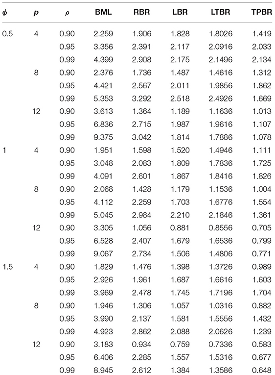
Table 1. Mean squared error (MSE) values for different estimators when n = 50.

TABLE 2

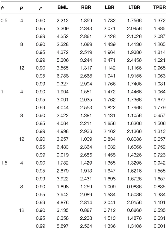
Table 2. Mean squared error values for different estimators when n = 100.

TABLE 3

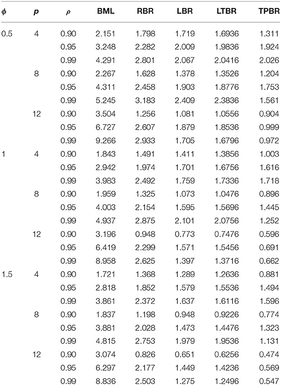
Table 3. Mean squared error values for different estimators when n = 250.

TABLE 4

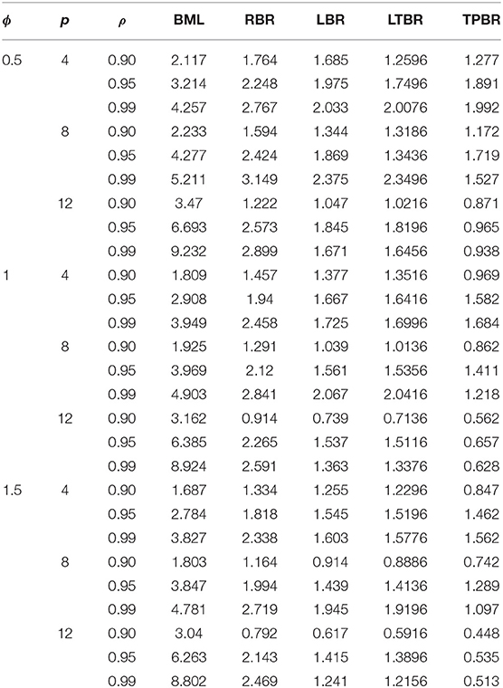
Table 4. Mean squared error values for different estimators when n = 400.

Relative Efficiency

Another comparative performance called relative efficiency (RE) can be utilized, it is calculated based on the MSE in Eq. (33) as follows [4, 39]:

$\begin{array}{ll}\text{RE}\left({\widehat{\beta }}_S\right)=\frac{MSE\left({\widehat{\beta }}_{BML}\right)}{MSE\left({\widehat{\beta }}_S\right)},& (34)\end{array}$

where ${\widehat{\beta }}_S$ denotes the estimators of RBR, LBR, LTBR, or TPBR. The RE results are shown in Figure 1.

FIGURE 1

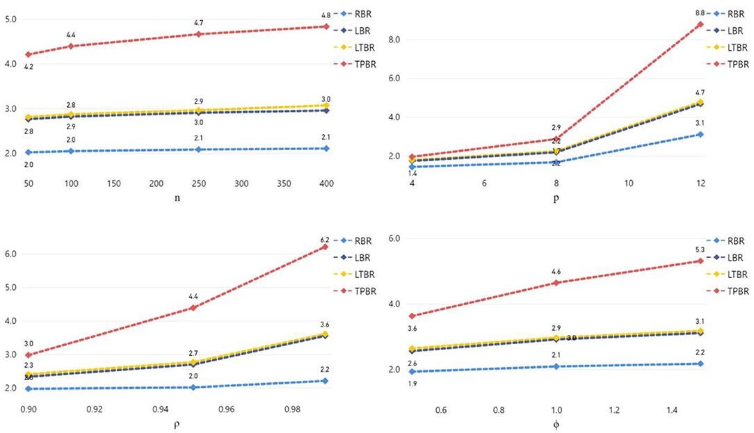
Figure 1. Relative efficiency (RE) of different estimators categorized by levels of n, p, ρ, and ϕ.

Figure 1 shows that the RE of the four biased (RBR, LBR, LTBR, and TPBR) estimators were increased if the sample size (n), the number of explanatory variables (p), the degree of correlation between explanatory variables (ρ), and/or the precision parameter value (ϕ) are increased. Moreover, we can observe that the TPBR estimator has higher RE values than the other estimators.

Real Data Applications

In this section, we used two real data applications to investigate the advantage of our proposed (TPBR) estimator in different fields.

Football Spanish Data

We apply the proposed estimator to the football Spanish La Liga, season 2016–2017 [19]. The data contain 20 teams. The response variable is the proportion of won matches. The six considerable explanatory variables are: x₁ is the number of yellow cards, x₂ is the number of red cards, x₃ is the total number of substitutions, x₄ is the number of matches with 2.5 goals on average, x₅ is the number of matches that ended with goals, and x₆ is the ratio of the goal scores to the number of matches.

First, to check whether there is a multicollinearity problem or not, the correlation matrix and condition number (CN) are used. Based on the correlation matrix among the six explanatory variables that are presented, displayed by Algamal and Abonazel [19]. It is obviously seen that there are correlations >0.82 between x₁ and x₆, x₁ and x₄, x₂ and x₄, and x₄ and x₆. Second, the condition number, $\text{CN}=\sqrt{{\lambda }_{\text{max}}/{\lambda }_{\text{min}}}$ of the data is 806.63 indicating the existence of multicollinearity. The estimated beta regression coefficients and MSE values for the BML, RBR, LBR, LTBR, and TPBR estimators are recorded in Table 5. From Table 5, it can note that the estimated coefficients of all estimators have the same signs; this means that the type of relationship between each explanatory variable and the response variable is not changed from what it was in the BML estimator. But MSE values of RBR, LBR, LTBR, and TPBR estimators are lower than the BML estimator. Whereas, the MSE value of the TPBR estimator is the lowest.

TABLE 5

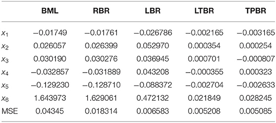
Table 5. The estimated coefficients and MSE values for the used estimators (football data).

Gasoline Yield Data

To further investigate the advantage of our proposed estimator (TPBR), we apply the TPBR estimator to the chemical dataset (gasoline yield data) which was originally obtained by Prater [42], and later used by the following authors: Ospina et al. [43] and Karlsson et al. [10]. The dataset contains 32 observations on the response and four explanatory variables. The variables in the study are described as follows: the dependent variable y is the proportion of crude oil after distillation and fractionation while the explanatory variables are crude oil gravity (Gravity), vapor pressure of crude oil (Pressure), temperature at which 10% of the crude oil has vaporized (Temp10), and temperature at which all petrol in the amount of crude oil vaporizes (Temp). Atkinson [44] analyzed this dataset using the linear regression model and observed some anomalies in the distribution of the error. Recently, Karlsson et al. [10] showed that the beta regression model is more suitable to model the data.

The CN for the dataset under study is 11,281.4, which signals severe multicollinearity. The estimated beta regression coefficients and MSE values for the used estimators are recorded in Table 6. From Table 6, it can be noted that the estimated coefficients of all estimators have the same signs. In addition, MSE values of RBR, LBR, LTBR, and TPBR estimators are lower than the BML estimator. Whereas, the MSE value of the TPBR estimator is the lowest.

TABLE 6

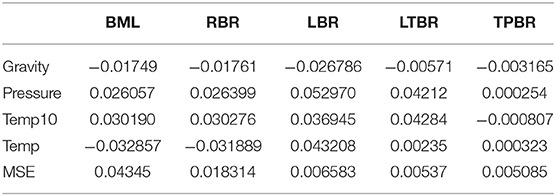
Table 6. The estimated coefficients and MSE values for the used estimators (gasoline yield data).

Conclusion

This article provided a two-parameter (TPBR) estimator for the beta regression model as a remedy for a multicollinearity problem. We proved, theoretically, that our proposed estimator is efficient than other biased estimators (ridge, Liu, and Liu-type estimators) suggested in the literature. Furthermore, a Monte Carlo simulation study was conducted to study the performance of the proposed estimator and ML, ridge, Liu, and Liu-type estimators. The results indicated that the proposed estimator outperforms these estimators, especially when there is a high-to-strong correlation between the explanatory variables. Finally, the benefit is shown by two empirical applications where the TPBR estimator performed well by decreasing the MSE compared with the ML, ridge, Liu, and Liu-type estimators.

For future work, for example, one can study the high-dimensional case in beta regression as an extension to Arashi et al. [45] or provide a robust biased estimation of beta regression as an extension to Awwad et al. [41] and Dawoud and Abonazel [40].

Data Availability Statement

Publicly available datasets were analyzed in this study. This data can be found at: For first application: https://www.laliga.es. For second application: the R-package betareg.

Author Contributions

MA: methodology, relative efficiency, interpreting the results, abstract, conclusions, writing—original draft, and final revision. ZA: simulation study and applications, interpreting the results, and revision. FA: methodology, interpreting the results, and revision. IT: introduction, methodology, and writing—original draft. All authors contributed to the article and approved the submitted version.

Conflict of Interest

The authors declare that the research was conducted in the absence of any commercial or financial relationships that could be construed as a potential conflict of interest.

Publisher's Note

All claims expressed in this article are solely those of the authors and do not necessarily represent those of their affiliated organizations, or those of the publisher, the editors and the reviewers. Any product that may be evaluated in this article, or claim that may be made by its manufacturer, is not guaranteed or endorsed by the publisher.

Acknowledgments

The authors would like to thank the Deanship of Scientific Research at King Saud University represented by the Research Center at CBA for supporting this research financially.

References

1. Hoerl AE, Kennard RW. Ridge regression: biased estimation for non-orthogonal problems. Technometrics. (1970) 12:55–67. doi: 10.1080/00401706.1970.10488634

CrossRef Full Text | Google Scholar

2. Hoerl AE, Kennard RW. Ridge regression: applications to non-orthogonal problems. Technometrics. (1970) 12:69–82. doi: 10.1080/00401706.1970.10488635

CrossRef Full Text | Google Scholar

3. Rady EA, Abonazel MR, Taha IM. Ridge estimators for the negative binomial regression model with application. In: The 53rd Annual Conference on Statistics, Computer Science, and Operation Research 3-5 Dec, 2018. (2018). Giza: ISSR, Cairo University.

Google Scholar

4. Abonazel MR, Taha IM. Beta ridge regression estimators: simulation and application. Commun Statist Simul Computat. (2021) 1–13. doi: 10.1080/03610918.2021.1960373

CrossRef Full Text | Google Scholar

5. Qasim M, Månsson K, Golam Kibria BM. On some beta ridge regression estimators: method, simulation and application. J Stat Comput Simul. (2021) 91:1699–712. doi: 10.1080/00949655.2020.1867549

CrossRef Full Text | Google Scholar

6. Alobaidi NN, Shamany RE, Algamal ZY. A new ridge estimator for the negative binomial regression model. Thailand Statistician. (2021) 19:116–25.

Google Scholar

7. Sami F, Amin M, Butt MM. On the ridge estimation of the Conway-Maxwell Poisson regression model with multicollinearity: Methods and applications. Concurr Computat Pract Exp. (2021) 2021:6477. doi: 10.1002/cpe.6477

PubMed Abstract | CrossRef Full Text | Google Scholar

8. Liu K. A new class of biased estimate in linear regression. Commun Statist Theor Method. (1993) 22:393–402. doi: 10.1080/03610929308831027

CrossRef Full Text | Google Scholar

9. Stein C. Inadmissibility of the usual estimator for the mean of a multivariate normal distribution. In: Proceedings of the Third Berkeley Symposium on Mathematical Statistics and Probability, Volume 1: Contributions to the Theory of Statistics. Berkeley, CA: University of California Press. (1956). p. 197–206. doi: 10.1525/9780520313880-018

PubMed Abstract | CrossRef Full Text

10. Karlsson P, Månsson K, Kibria BG. A Liu estimator for the beta regression model and its application to chemical data. J Chemom. (2020) 34:e3300. doi: 10.1002/cem.3300

PubMed Abstract | CrossRef Full Text | Google Scholar

11. Qasim M, Kibria BMG, Månsson K, Sjölander P. A new Poisson Liu regression estimator: method and application. J Appl Stat. (2020) 47:2258–71. doi: 10.1080/02664763.2019.1707485

CrossRef Full Text | Google Scholar

12. Naveed K, Amin M, Afzal S, Qasim M. New shrinkage parameters for the inverse Gaussian Liu regression. Commun Statist Theor Method. (2020) 2020:1–21. doi: 10.1080/03610926.2020.1791339

CrossRef Full Text | Google Scholar

13. Liu K. Using Liu-type estimator to combat collinearity. Commun Statist Theor Method. (2003) 32:1009–20. doi: 10.1081/STA-120019959

PubMed Abstract | CrossRef Full Text | Google Scholar

14. Liu K. More on Liu-type estimator in linear regression. Commun Statist Theor Method. (2004) 33:2723–33. doi: 10.1081/STA-200037930

PubMed Abstract | CrossRef Full Text | Google Scholar

15. Özkale MR, Kaciranlar S. The restricted and unrestricted two-parameter estimators. Commun Stat Theor Method. (2007) 36:2707–25. doi: 10.1080/03610920701386877

CrossRef Full Text | Google Scholar

16. Li Y, Yang H. A new Liu-type estimator in linear regression model. Stat Pap. (2012) 53:427–37. doi: 10.1007/s00362-010-0349-y

CrossRef Full Text | Google Scholar

17. Kurnaz FS, Akay KU. A new Liu-type estimator. Stat Pap. (2015) 56:495–517. doi: 10.1007/s00362-014-0594-6

CrossRef Full Text | Google Scholar

18. Sahriman S, Koerniawan V. Liu-type regression in statistical downscaling models for forecasting monthly rainfall salt as producer regions in Pangkep regency. J Phys Conf Ser. (2019) 1341:092021. doi: 10.1088/1742-6596/1341/9/092021

CrossRef Full Text | Google Scholar

19. Algamal ZY, Abonazel MR. Developing a Liu-type estimator in beta regression model. Concurr Computat Pract Exp. (2021) 2021:e6685. doi: 10.1002/cpe.6685

PubMed Abstract | CrossRef Full Text | Google Scholar

20. Huang J, Yang H. A two-parameter estimator in the negative binomial regression model. J Stat Comput Simul. (2014) 84:124–34. doi: 10.1080/00949655.2012.696648

PubMed Abstract | CrossRef Full Text | Google Scholar

21. Algamal ZY. Shrinkage estimators for gamma regression model. Electr J Appl Stat Anal. (2018) 11:253–68. doi: 10.1285/i20705948v11n1p253

PubMed Abstract | CrossRef Full Text | Google Scholar

22. Asar Y, Genç A. A new two-parameter estimator for the Poisson regression model. Iran J Sci Technol Trans A Sci. (2018) 42:793–803. doi: 10.1007/s40995-017-0174-4

CrossRef Full Text | Google Scholar

23. Rady EA, Abonazel MR, Taha IM. A new biased estimator for zero-inflated count regression models. J Modern Appl Stat Method. (2019). Available online at: https://www.researchgate.net/publication/337155202_A_New_Biased_Estimator_for_Zero-Inflated_Count_Regression_Models

Google Scholar

24. Rady EA, Abonazel MR, Taha IM. New shrinkage parameters for Liu-type zero inflated negative binomial estimator. In: The 54th Annual Conference on Statistics, Computer Science, and Operation Research 3-5 Dec, 2019. Giza: FGSSR, Cairo University (2019).

Google Scholar

25. Çetinkaya M, Kaçiranlar S. Improved two-parameter estimators for the negative binomial and Poisson regression models. J Stat Comput Simul. (2019) 89:2645–60. doi: 10.1080/00949655.2019.1628235

CrossRef Full Text | Google Scholar

26. Abonazel MR, Farghali RA. Liu-type multinomial logistic estimator. Sankhya B. (2019) 81:203–25. doi: 10.1007/s13571-018-0171-4

CrossRef Full Text | Google Scholar

27. Akram MN, Amin M, Qasim M. A new Liu-type estimator for the Inverse Gaussian Regression Model. J Stat Comput Simul. (2020) 90:1153–72. doi: 10.1080/00949655.2020.1718150

CrossRef Full Text | Google Scholar

28. Lukman AF, Aladeitan B, Ayinde K, Abonazel MR. Modified ridge-type for the Poisson regression model: simulation and application. J Appl Stat. (2021) 2021:1–13. doi: 10.1080/02664763.2021.1889998

CrossRef Full Text | Google Scholar

29. Ferrari S, Cribari-Neto F. Beta regression for modelling rates and proportions. J Appl Stat. (2004) 31:799–815. doi: 10.1080/0266476042000214501

CrossRef Full Text | Google Scholar

30. Smithson M, Verkuilen J. A better lemon squeezer? Maximum-likelihood regression with beta-distributed dependent variables. Psychol Method. (2006) 11:54–71. doi: 10.1037/1082-989X.11.1.54

PubMed Abstract | CrossRef Full Text | Google Scholar

31. Cribari-Neto F, Zeileis A. Beta regression in R. J Stat Softw. (2010) 34:1–24. doi: 10.18637/jss.v034.i02

CrossRef Full Text | Google Scholar

32. Bayer FM, Cribari-Neto F. Model selection criteria in beta regression with varying dispersion. Commun Stat Simul Computat. (2017) 46:729–46. doi: 10.1080/03610918.2014.977918

CrossRef Full Text | Google Scholar

33. Espinheira PL, Ferrari SL, Cribari-Neto F. On beta regression residuals. J Appl Stat. (2008) 35:407–19. doi: 10.1080/02664760701834931

CrossRef Full Text | Google Scholar

34. Espinheira PL, da Silva LCM, Silva ADO. Prediction measures in beta regression models. arXiv preprint. (2015). arXiv: 1501.04830.

Google Scholar

35. Espinheira PL, da Silva LCM, Silva ADO, Ospina R. Model selection criteria on beta regression for machine learning. Machine Learn Knowl Extr. (2019) 1:427–49. doi: 10.3390/make1010026

PubMed Abstract | CrossRef Full Text | Google Scholar

36. Farebrother RW. Further results on the mean square error of ridge regression. J Royal Stat Soc Ser B. (1976) 38:248–50. doi: 10.1111/j.2517-6161.1976.tb01588.x

CrossRef Full Text | Google Scholar

37. Hoerl AE, Kennard RW, Baldwin KF. Ridge regression: some simulations. Commun Stat Theor Method. (1975) 4:105–23. doi: 10.1080/03610917508548342

CrossRef Full Text | Google Scholar

38. Kibria BMG. Performance of some new ridge regression estimators. Commun Stat Simul Computat. (2003) 32:419–35. doi: 10.1081/SAC-120017499

PubMed Abstract | CrossRef Full Text | Google Scholar

39. Farghali RA, Qasim M, Kibria BG, Abonazel MR. Generalized two-parameter estimators in the multinomial logit regression model: methods, simulation and application. Commun Stat Simul Computat. (2021) 1–16. doi: 10.1080/03610918.2021.1934023

CrossRef Full Text | Google Scholar

40. Dawoud I, Abonazel MR. Robust Dawoud–Kibria estimator for handling multicollinearity and outliers in the linear regression model. J Stat Comput Simul. (2021) 91:3678–92. doi: 10.1080/00949655.2021.1945063

CrossRef Full Text | Google Scholar

41. Awwad FA, Dawoud I, Abonazel MR. Development of robust Özkale-Kaçiranlar and Yang-Chang estimators for regression models in the presence of multicollinearity and outliers. Concurr Computat Pract Exp. (2021) 2021:e6779. doi: 10.1002/cpe.6779

PubMed Abstract | CrossRef Full Text | Google Scholar

42. Prater NH. Estimate gasoline yields from crude. PetroLium Refiner. (1956) 35:236–8.

43. Ospina R, Cribari-Neto F, Vasconcellos KL. Improved point and interval estimation for a beta regression model. Comput Stat Data Anal. (2006) 51:960–81. doi: 10.1016/j.csda.2005.10.002

PubMed Abstract | CrossRef Full Text | Google Scholar

44. Atkinson AC. Plots, Transformations and Regression: An Introduction to Graphical Methods of Diagnostic Regression Analysis. New York, NY: Oxford University Press (1985).

Google Scholar

45. Arashi M, Norouzirad M, Roozbeh M, Mamode Khan N. A high-dimensional counterpart for the ridge estimator in multicollinear situations. Mathematics. (2021) 9:3057. doi: 10.3390/math9233057

CrossRef Full Text | Google Scholar