An Empirical Study of Graph-Based Approaches for Semi-supervised Time Series Classification

1. Introduction

Many processes for which data are collected are time-dependent and as a result the study of time series data is a subject of great importance [1–3]. The case of time series is interesting for tasks such as anomaly detection [4], motif computation [5] or time series forecasting [6]. We refer to [7–10] for more general introductions.

We here focus on the task of classification of time series [11–16] in the context of semi-supervised learning [17, 18] where we want to label all data points¹ based on the fact that only a small portion of the data is already pre-labeled.

An example is given in Figure 1 where we see some time series reflecting ECG (electrocardiogram) data and the classification into normal heartbeats on the one hand and myocardial infarction on the other hand. In our applications, we assume that only for some of the time series the corresponding class is known a priori. Our main contribution is to introduce a novel combination of incorporating the data into a graph and then incorporate this representation into several recently introduced methods for semi-supervised learning. For this, each time series becomes a node within a weighted undirected graph and the edge-weight is proportional to the similarity between different time series. Graph-based approaches have become a standard tool in many learning tasks (cf. [19–24] and the references mentioned therein). The matrix representation of the graph via its Laplacian [25] leads to studying the network using matrix properties. The Laplacian is the representation of the network that is utilized from machine learning to mathematical imaging. Recently, it has also been used network-Lasso-based learning approaches focusing on data with an inherent network structure, see e.g., [26, 27]. A very important ingredient in the construction of the Laplacian is the choice of the appropriate weight function. In many applications, the computation of the distance between time series or sub-sequences becomes a crucial task and this will be reflected in our choice of weight function. We consider several distance measures such as dynamic time warping DTW [28], soft DTW [29], and matrix profile [30].

FIGURE 1

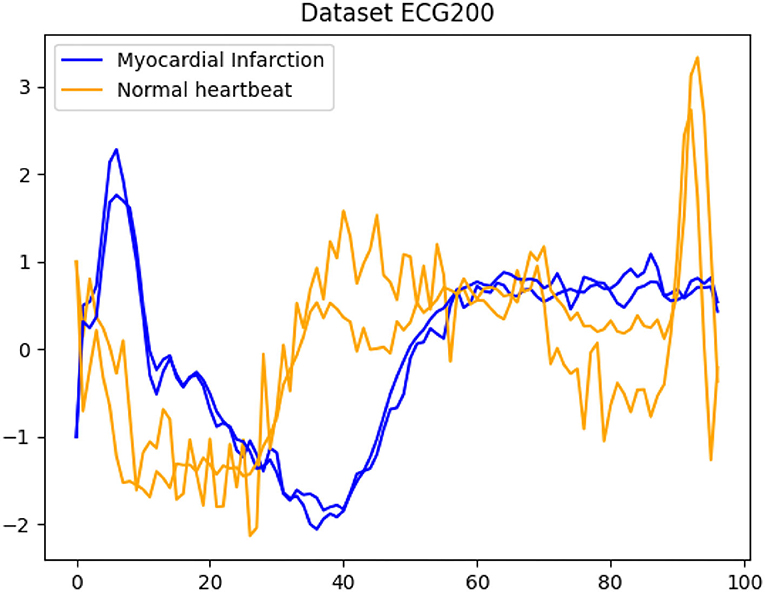
Figure 1. A typical example for time series classification. Given the dataset ECG200, the goal is to automatically separate all time series into the classes normal heartbeats and myocardial infarction.

We will embed these measures via the graph Laplacian into two different recently proposed semi-supervised learning frameworks. Namely, a diffuse interface approach that originates from material science [31] via the graph Allen-Cahn equation as well as a method based on graph convolutional networks [21]. Since these methods have originally been introduced outside of the field of time series learning, their relationship with time series distance measures has never been studied. Our goal is furthermore to compare these approaches with the well-known 1NN approach [11] and a simple optimization formulation solved relying on a linear system of equations. Our motivation follows that of [32, 33], where many methods for supervised learning in the context of time series were compared, namely that we aim to provide a wide-ranging overview of recent methods based on a graph representation of the data and combined with several distance measures.

We structure the paper as follows. In section 2, we introduce some basic notations and illustrate the basic notion of graph-based learning motivated with a clustering approach. In section 3, we discuss several distance measures with a focus on the well-known DTW measure as well as two recently emerged alternatives, i.e., Soft DTW and the MP distance. We use section 4 to introduce the two semi-supervised learning methods in more detail, followed by a shorter description of their well-known competitors. section 5 will allow us to compare the methods and study the hyperparameter selection.

2. Basics

We consider discrete time series x_i given as a vector of real numbers of length m_i. In general, we allow for the time series to be of different dimensionality; later we often consider all m_i = m. We assume that we are given n time series ${\text{x}}_i\in {ℝ}^{m_i}$. The goal of a classification task is to group the n time series into a number k of different clusters C_j with j = 1, …, k. In this paper we focus on the task of semi-supervised learning [17] where only some of the data are already labeled but we want to classify all available data simultaneously. Nevertheless, we review some techniques for unsupervised learning first as they deliver useful terminology. As such the k-means algorithm is a prototype-based² clustering algorithm that divides the given data into a predefined number of k clusters [34]. The idea behind k-means is rather simple as the cluster centroids are repeatedly updated and the data points are assigned to the nearest centroid until the centroids and data points have converged. Often the termination condition is not handled that strictly. For example, the method can be terminated when only 1% of the points change clusters. The starting classes are often chosen at random but can also be assigned in a more systematic way by calculating the centers first and then assign the points to the nearest center. While k-means remains very popular it also has certain weaknesses coming from its minimization of the sum of squared errors loss function [35]. We discuss this method in some detail here to point out the main mechanism and this is based on assigning points to clusters and hence the cluster centroids based on the distance being the Euclidean norm, which would also be done when k-means is applied to time series. As a result the clusters might not capture the shape of the data manifold as illustrated in a simple two-dimensional example shown in Figure 2. In comparison, the alternative method shown, i.e., a spectral clustering technique, performs much better. We briefly discuss this method next as it forms the basis of the main techniques introduced in this paper.

FIGURE 2

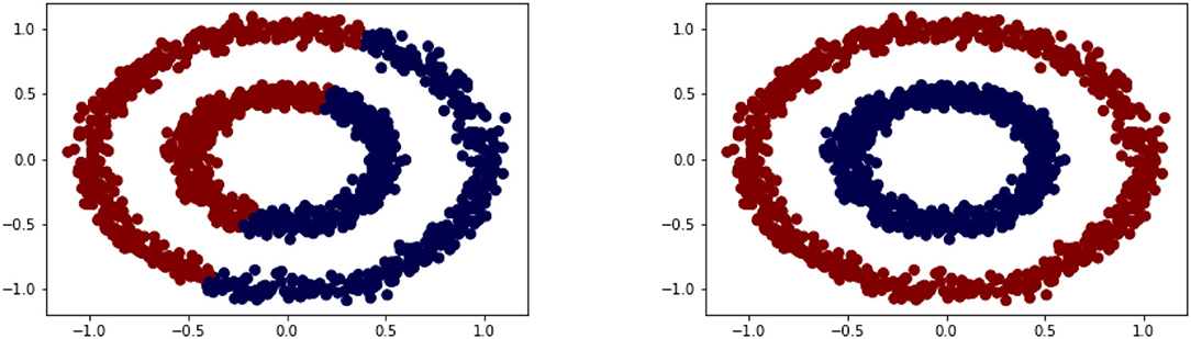
Figure 2. Clustering based on original data via k-means (left) vs. transformed data via spectral clustering (right).

2.1. Graph Laplacian and Spectral Clustering

As we illustrated in Figure 2 the separation of the data into two-classes is rather difficult for k-means as the centroids are based on a 2-norm minimization. One alternative to k-means is based on interpreting the data points as nodes in a graph. For this, we assume that we are given data points x₁, …, x_n and some measure of similarity [23]. We define the weighted undirected similarity graph G = (V, E) with the vertex or node set V and the edge set E. We view the data points x_i as vertices, V = {x₁, …, x_n}, and if two nodes (x_i, x_j) have a positive similarity function value, they are connected by an edge with weight w_ij equal to that similarity. With this reformulation of the data we turn the clustering problem into a graph partitioning problem where we want to cut the graph into two or possibly more classes. This is usually done in such a way that the weight of the edges across the partition is minimal.

We collect all edge weights in the adjacency matrix W = (_{wij)i, j = 1, …, n}. The degree of a vertex x_i is defined as $d_i=\sum _{j=1}^n{w}_{ij}$ and the degree matrix D is the diagonal matrix holding all n node degrees. In our case we use a fully connected graph with the Gaussian similarity function

$\begin{array}{ll}w({\text{x}}_i,{\text{x}}_j)=exp{\displaystyle (-\frac{\text{dist}{({\text{x}}_i,{\text{x}}_j)}^2}{{\sigma }^2})},& (1)\end{array}$

where σ is a scaling parameter and dist(x_i, x_j) is a particular distance function such as the Euclidean distance $\mathrm{\text{dist}}({\text{x}}_i,{\text{x}}_j):=\parallel {\text{x}}_i-{\text{x}}_j{\parallel }^2$. Note that for similar nodes, the value of the distance function is smaller than it would be for dissimilar nodes while the similarity function is relatively large.

We now use both the degree and weight matrix to define the graph Laplacian as L = D − W. Often the symmetrically normalized Laplacian defined via

$\begin{array}{ll}{L}_{\text{sym}}=D^{-\frac{1}{2}}L{D}^{-\frac{1}{2}}=I-D^{-\frac{1}{2}}W{D}^{-\frac{1}{2}}& (2)\end{array}$

provides better clustering information [23]. It has some very useful properties that we will exploit here. For example, given a non-zero vector u ∈ ℝⁿ we obtain the energy term

$\begin{array}{ll}\begin{array}{c}{u}^T{L}_{\text{sym}}u=\frac{1}{2}{\displaystyle \sum _{i,j}}{w}_{ij}{\left(\frac{u_i}{\sqrt{d_i}}-\frac{u_j}{\sqrt{d_j}}\right)}^2.\hfill \end{array}& (3)\end{array}$

Using this it is easy to see that L_sym is positive semi-definite with non-negative eigenvalues 0 = λ₁ ≤ λ₂ ≤… ≤ λ_n. The main advantage of the graph Laplacian is that based on its spectral information one can usually rely on transforming the data into a space where they are easier to separate [23, 25, 36]. As a result one typically requires the spectral information corresponding to the smallest eigenvalues of L_sym. The most famed eigenvector is the Fiedler vector, i.e., the eigenvector corresponding to the first non-zero eigenvalue, which is bound to have a sign change and as a result can be used for binary classification. The weight function (1) is also found in kernel methods [37, 38] when the radial basis kernel is applied.

2.2. Self-Tuning

In order to improve the performance of the methods based on the graph Laplacian, tuning the parameter σ is crucial. While hyperparameter tuning based on a grid search or cross validation is certainly possible we also consider a σ that adapts to the given data. For spectral clustering, such a procedure was introduced in [39]. Here we use this technique to learning with time series data. For each time series x_i we assume a local scaling parameter σ_i. As a result, we have the generalized square distance as

$\begin{array}{ll}\begin{array}{c}\frac{\text{dist}({\text{x}}_i,{\text{x}}_j)}{{\sigma }_i}\frac{\text{dist}({\text{x}}_i,{\text{x}}_j)}{{\sigma }_j}=\frac{\text{dist}{({\text{x}}_i,{\text{x}}_j)}^2}{{\sigma }_i{\sigma }_j}\hfill \end{array}& (4)\end{array}$

and this gives the entries of the adjacency matrix W via

$\begin{array}{ll}\begin{array}{c}{w}_{i,j}=exp\left(-\frac{\text{dist}{({\text{x}}_i,{\text{x}}_j)}^2}{{\sigma }_i{\sigma }_j}\right).\hfill \end{array}& (5)\end{array}$

The authors in [39] choose σ_i as the distance to the K-th nearest neighbor of x_i where K is a fixed parameter, e.g., K = 9 is used in [31].

In section 5, we will explore several different values for K and their influence on the classification behavior.

3. Distance Measures

We have seen from the definition of the weight matrix that the Laplacian depends on the choice of distance measure dist(x_i, x_j). If all time series are of the same length then the easiest distance measure would be a Euclidean distance, which especially for large n is fast to compute. This makes the Euclidean distance incredibly popular but it suffers from being sensitive to small shifts in the time series. As a result we discuss several popular and efficient methods for different distance measures. Our focus is to illustrate in an empirical study how the choice of distance measure impacts the performance of graph-based learning and to provide further insights for future research (cf. [40]).

3.1. Dynamic Time Warping

We first discuss the distance measure of Dynamic Time Warping (DTW, [28]). By construction, DTW is an algorithm to find an optimal alignment between time series.

In the following, we adapt the notation of [28] to our case. Consider two time series x and $\tilde{x}$ of lengths m and $\tilde{m}$, respectively, with entries $x_i,{\tilde{x}}_i\in ℝ$ for i = 1, …, m and $j=1,\dots ,\tilde{m}$. We obtain the local cost matrix $C\in {ℝ}^{m\times \tilde{m}}$ by assembling the local differences for each pair of elements, i.e., $C_{ij}=|x_i-{\tilde{x}}_j|$.

The DTW distance is defined via $(m,\tilde{m})$-warping paths, which are sequences of index tuples p = ((i₁, j₁), …, (i_L, j_L)) with boundary, monotonicity, and step size conditions

$\begin{array}{l}\hfill 1=i_1\le i_2\le \dots \le i_L=m,1=j_1\le j_2\le \dots \le \tilde{m},\hfill \\ \hfill (i_{\ell +1}-i_{\ell },j_{\ell +1}-j_{\ell })\in \left\{(1,0),(0,1),(1,1)\right\}(\ell =1,\dots ,L-1).\hfill \end{array}$

The total cost of such a path with respect to x, $\tilde{x}$ is defined as

$c_p(\text{x},\tilde{\text{x}})={\displaystyle \sum _{\ell =1}^L}|x_{i_{\ell }}-{\tilde{x}}_{j_{\ell }}|.$

The DTW distance is then defined as the minimum cost of any warping path:

$\begin{array}{ll}\text{DTW}(\text{x},\text{y}):=min\left\{c_p(\text{x},\text{y})\mid p\text{is a (m,}\tilde{m}\text{)-warping path}\right\}.& (6)\end{array}$

Both the warping and the warping path are illustrated in Figure 3.

FIGURE 3

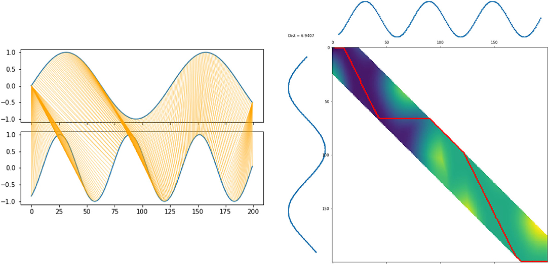
Figure 3. DTW warping (left) and warpings paths (right).

Computing the optimal warping path directly quickly becomes infeasible. However, we can use dynamic programming to evaluate the accumulated cost matrix D recursively via

$\begin{array}{ll}D(i,j):=|x_i-{\tilde{x}}_j|+min\left\{D(i,j-1),D(i-1,j),D(i-1,j-1)\right\}.& (7)\end{array}$

The actual DTW distance is finally obtained as

$\begin{array}{ll}\text{DTW}(\text{x},\text{y})=D(m,\tilde{m}).& (8)\end{array}$

The DTW method is a heavily used distance measure for capturing the sometimes subtle similarities between time series. In the literature it is typically stated that the computational cost of DTW being prohibitively large. As a result one is interested in accelerating the DTW algorithm itself. One possibility arises from imposing additional constraints (cf. [28, 41]) such as the Sakoe-Chiba Band and the Itakura parallelogram as these simplify the identification of the optimal warping path. While these are appealing concepts the authors in [42] observe that the well-known FastDTW algorithm [41] is in fact slower than DTW. For our purpose we will hence rely on DTW and in particular on the implementation of DTW provided via https://github.com/wannesm/dtaidistance. We observe that for this implementation of DTW indeed FastDTW is outperformed frequently.

3.2. Soft Dynamic Time Warping

Based on a slight reformulation of the above DTW scheme, we want to look at another time series distance measure, the Soft Dynamic Time Warping (Soft DTW). It is an extension of DTW designed allowing a differentiable loss function and it was introduced in [29, 43]. We again start from the cost matrix C with $C(i,j)=|x_i-{\tilde{x}}_j|$ for time series x and $\tilde{x}$. Each warping path can equivalently be described by a matrix $A\in {\left\{0,1\right\}}^{m\times \tilde{m}}$ with the following condition: The ones in A form a path starting in (1, 1) going to $(m,\tilde{m})$, only using steps downwards, to the right and diagonal downwards. A is called monotonic alignment matrix and we denote the set containing all these alignment matrices with ${A}(m,\tilde{m})$. The Frobenius inner product 〈A, C〉 is then the sum of costs along the alignment A. Solving the following minimization problem leads us to a reformulation of the dynamic time warping introduced above as

$\begin{array}{ll}\text{DTW}(C)={\displaystyle \underset{A\in {A}(N,M)}{min}}\langle A,C\rangle .& (9)\end{array}$

With Soft DTW we involve all alignments possible in ${A}(N,M)$ by replacing the minimization with a soft minimum:

$\begin{array}{ll}{\displaystyle \underset{x\in S}{min}}f(x)\approx {{\text{min}}_{\gamma }}_{x\in S}f(x):=-\gamma log{\displaystyle \sum _{x\in S}}exp\left(\frac{-f(x)}{\gamma }\right)& (10)\end{array}$

where S is a discrete subset of the real numbers. This function approximates the minimum of f(x) and is differentiable. The parameter γ controls the tuning between smoothness and approximation of the minimum. Using the DTW-function (9) within (10) yields the expression for Soft Dynamic Time Warping written as

$\begin{array}{l}{\text{DTW}}_{\gamma }(\text{x},\tilde{\text{x}})={{\text{min}}_{\gamma }}_{A\in {A}(m,n)}\langle A,C\rangle \\ =-\gamma log{\displaystyle \sum _{A\in {A}(m,n)}}exp\left(\frac{-\langle A,C\rangle }{\gamma }\right).& (11)\end{array}$

This is now a differentiable alternative to DTW, which involves all alignments in our cost matrix.

Due to entropic bias³, Soft DTW can generate negative values, which would cause issues for our use in time series classification. We apply the following remedy to overcome this drawback:

$\begin{array}{ll}\text{Div}(\text{x},\text{y})={\text{DTW}}_{\gamma }(\text{x},\text{y})-\frac{1}{2}·{\displaystyle ({\text{DTW}}_{\gamma }(\text{x},\text{x})+{\text{DTW}}_{\gamma }(\text{y},\text{y}))}.& (12)\end{array}$

This measure is called Soft DTW divergence [43] and will be employed in our experiments.

3.3. Matrix Profile Distance

Another alternative time series measure that has recently been introduced is the Matrix Profile Distance (MP distance, [30]). This measure is designed for fast computation and finding similarities between time series.

We will again introduce the concept of the matrix profile of two time series x and $\tilde{x}$. The matrix profile is based on the subsequences of these two time series. For a fixed window length L, the subsequence x_i,L of a time series x is defined as a contiguous L-element subset of x via x_i,L = (x_i, x_{i + 1}, …, x_i+L−1). The all-subsequences set A of x contains all possible subsequences of x with length L, A = {x_1,L, x_2,L, …, x_{m−L + 1, L}}, where m is again the length of x.

For the matrix profile, we need the all-subsequences sets A and B of both time series x and $\tilde{x}$. The matrix profile P_ABBA is the set consisting of the closest Euclidean distances from each subsequence in A to any subsequence in B and vice versa:

$\begin{array}{c}{\text{P}}_{\text{ABBA}}=\left\{{\displaystyle \underset{{\tilde{\text{x}}}_{j,L}\in B}{min}}||{\text{x}}_{i,L}-{\tilde{\text{x}}}_{j,L}|||{\text{x}}_{i,L}\in A\right\}\cup \\ \left\{{\displaystyle \underset{{\text{x}}_{i,L}\in A}{min}}||{\tilde{\text{x}}}_{j,L}-{\text{x}}_{i,L}|||{\tilde{\text{x}}}_{j,L}\in B\right\}\end{array}$

With the matrix profile, we can finally define the MP distance based on the idea that two time series are similar if they have many similar subsequences. We do not consider the smallest or the largest value of P_ABBA because then the MP distance could be too rough or too detailed. For example, if we would have two rather similar time series, but either one has a noisy spike or some missing values, then the largest value of the matrix profile could give a wrong impression about the similarity of these two time series. Instead, the distance is defined as

$\text{MPdist}(X,Y)=k\text{-th smallest value in sorted }{\text{P}}_{ABBA},$

where the parameter k is typically set to 5% of 2N [30].

We now illustrate the MP distance using an example as illustrated in section 3.3, where we display three time series of length N = 100. Our goal is to compare these time series using the MP distance. We observe that X₁ and X₂ have quite similar oscillations. The third time series X₃ does not share any obvious features with the first two sequences.

The MP distance compares the subsequences of the time series, depending on the window length L. Choosing the window length to be L = 40, we get the following distances:

$\begin{array}{l}\begin{array}{c}\text{MPdist}(X_1,X_2)=0.433,\\ \text{MPdist}(X_1,X_3)=5.425,\\ \text{MPdist}(X_2,X_3)=5.404.\end{array}\end{array}$

As we can see, the MP distance identified the similarity between X₁ and X₂ shows that X₁, X₂ differ from X₃. We also want to show that the MP Distance depends on the window length L. Let us look at the MP distance between the lower oscillation time series X₂ and X₃, which is varying a lot for different values of L as indicated in Table 1. Choosing L = 10 there is not a large portion of both time series to compare with and as a result we observe a small value for the MP distance, which does not describe the dissimilarity of X₂ and X₃ in a proper way. If we look at L = 40, there is a larger part of the time series structure to compare the two series. If there is a special recurring pattern in the time series, the length L should be large enough to cover one recurrence. We illustrate the comparison based on different window lengths in Figure 4.

TABLE 1

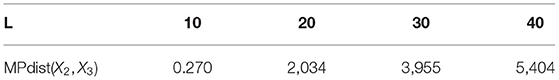
Table 1. MP distance depending on the window length.

FIGURE 4

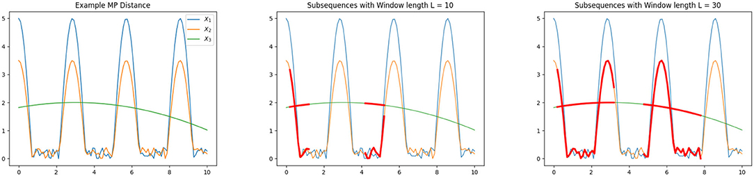
Figure 4. Illustration of Matrix Profile distance (left), subsequences indicated in red with window length L = 10 (middle) and L = 30 (right).

For the tests all data sets consist of time series with a certain length, varying for each data set. Thus we have to decide which window length L should be chosen automatically in the classifier. An empirical study showed that choosing L ≈ N/2 gives good classification results.

We briefly illustrate the computing times of the different distance measures when applied to time series of increasing length shown in Figure 5. It can be seen that DTW is faster than fastDTW. Obviously, the Euclidean distance shows the best scalability. We also observe that the computation of the SDTW is scaling worse than the competing approaches when applied to longer time series.

FIGURE 5

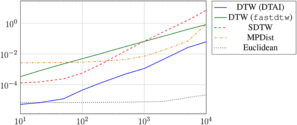
Figure 5. Runtimes of distance computation between a single pair of time series with increasing length.

4. Semi-Supervised Learning Based on Graph Laplacians

In this section, we focus mainly on two methods that have recently gained wide attention. This first method is inspired by a partial differential equation model originating from material science and the second approach is based on neural networks that incorporate the graph structure of the labeled and unlabeled data.

4.1. Semi-supervised Learning With Phase Field Methods: Allen–Cahn Model

Within the material science community phase field methods have been developed to model the phase separation of a multicomponent alloy system (cf. [45, 46]). The evolution of the phases over time is described by a partial differential equation (PDE) model, such as the Allen-Cahn [46] or Cahn-Hilliard equation [47] both non-linear reaction-diffusion equations of second and fourth order, respectively. These equations can be obtained as gradient flows of the Ginzburg–Landau energy functional

${\displaystyle {E}(u)=\int \frac{\epsilon }{2}|\nabla u{|}^2+\frac{1}{\epsilon }\varphi (u)}$

where u is the order parameter and ε a parameter reflecting the width of the interface between the pure phases. The polynomial ϕ is chosen to have minima at the pure phases, namely u = −1 and u = 1, to enforce that a minimization of the Ginzburg–Landau energy will lead to phase separation. A common choice is the well-known double-well potential $\varphi (u)=\frac{1}{4}{(1-u^2)}^2.$ The Dirichlet energy term |∇u|² corresponds to minimization of the interfacial length. The minimization is then performed using a gradient flow, which leads to the Allen-Cahn equation

$\begin{array}{ll}{u}_t=\Delta u-\frac{1}{\epsilon }{\varphi }^{\prime }(u)& (13)\end{array}$

equipped with appropriate boundary and initial conditions. A modified Allen–Cahn equation was used for image inpainting, i.e., restoring damage parts in an image, where a misfit ω(f−u) term is added to Equation (13) (cf. [48, 49]). Here, ω is a penalty parameter and f is a function equal to the undamaged image parts or later training data. In [31], Bertozzi and Flenner extended this idea to the case of semi-supervised learning where the training data correspond to the undamaged image parts, i.e, the function f. Their idea is to consider the modified energy of the following form

$\begin{array}{ll}E(u)=\frac{\epsilon }{2}{u}^T{L}_{\text{sym}}u+\frac{1}{4\epsilon }{\displaystyle \sum _{i=1}^n}{(u_i^2-1)}^2+{\displaystyle \sum _{i=1}^n}\frac{{\omega }_i}{2}(f_i-u_i)& (14)\end{array}$

where f_i holds the already assigned labels. Here, the first term in (14) reflects the RatioCut based on the graph Laplacian, the second term enforces the pure phases, and the third term corresponds to incorporating the training data. Numerically, this system is solved using a convexity splitting approach [31] where we write

$E(u)=E_1(u)-E_2(u)$

with

$E_1(u):=\frac{\epsilon }{2}{u}^T{L}_{\text{sym}}u+\frac{c}{2}{u}^{T}u$

and

$E_2(u):=\frac{c}{2}{u}^{T}u-\frac{1}{4\epsilon }+{\displaystyle \sum _{i=1}^n}{(u_i^2-1)}^2-{\displaystyle \sum _{i=1}^n}\frac{{\omega }_i}{2}(f_i-u_i)$

where the positive parameter c ∈ ℝ ensures convexity of both energies. In order to compute the minimizer of the above energy we use a gradient scheme where

$\frac{u^{l+1}-u^l}{\tau }=-\nabla E_1(u^{l+1})+\nabla E_2(u^l)$

where the indices k, k + 1 indicate the current and next time step, respectively. The variable τ is a hyperparameter but can be interpreted as a pseudo time-step. In more detail following the notation of [20], this leads to

$\frac{u^{l+1}-u^l}{\tau }+\epsilon L_{\text{sym}}{u}^{l+1}+c{u}^{l+1}=c{u}^l-\frac{1}{\epsilon }\nabla \psi (u^l)+\nabla \varphi (u^l)$

with

$\psi (u^l)={\displaystyle \sum _{i=1}^n}{({(u_i^l)}^2-1)}^2,\varphi (u^l)={\displaystyle \sum _{i=1}^n}\frac{{\omega }_i}{2}(f_i-u_i^l).$

Expanding the order parameter in a number of the small eigenvectors ϕ_i of L_sym via $u=\sum _{i=1}^{m_e}{a}_i{\varphi }_i={\Phi }_{m_e}a$ where a is a coefficient vector and Φ_me = [ϕ₁, …, ϕ_me]. This lets us arrive at

$(1+\epsilon \tau {\lambda }_j{a}_j^{l+1}+c\tau )a_j^{l+1}=(1+\tau c)a_j^l-\frac{1}{\epsilon }{b}_j^l+d_j^l,\forall j=1,\dots ,m_e$

using

$b^l={\Phi }_{m_e}^T\nabla \psi ({\Phi }_{m_e}{a}^l),d^l={\Phi }_{m_e}^T\nabla \varphi ({\Phi }_{m_e}{a}^l).$

In [50], the authors extend this to the case of multiple classes where again the spectral information of the graph Laplacian are crucial as the energy term includes $\frac{\epsilon }{2}\mathrm{\text{tr}}(U^T{L}_{\mathrm{\text{sym}}}U)$ with U ∈ ℝ^{n, s}, s being the number of classes for segmentation, and tr being the trace of the matrix. Details of the definition of the potential and the fidelity term incorporating the training data are found in [50]. Further extensions of this approach have been suggested in [20, 22, 51–55].

4.2. Semi-supervised Learning Based on Graph Convolutional Networks

Artificial neural networks and in particular deep neural networks have shown outstanding performance in many learning tasks [56, 57]. The incorporation of additional structural information via a graph structure has received wide attention [24] with particular success within the semi-supervised learning formulation [21].

Let ${\text{h}}_i^{(l)}$ denote the hidden feature vector of the i-th node in the l-th layer. The feature mapping of a simple multilayer perceptron (MLP) computes the new features by multiplying with a weight matrix Θ^(l)T and adding a bias vector b^(l), then applying a (potentially layer-dependent) ReLU activation function σ_l in all layers except the last. This layer operation can be written as ${\text{h}}_i^l={\sigma }_l{\displaystyle ({\Theta }^{(l)T}{\text{h}}_i^{(l-1)}+{\text{b}}^{(l)})}$.

In Graph Neural Networks, the features are additionally propagated along the edges of the graph. This is achieved by forming weighted sums over the local neighborhood of each node, leading to

$\begin{array}{ll}{\text{h}}_i^l={\sigma }_l({\displaystyle \sum _{j\in {{N}}_i\cup \left\{i\right\}}}\frac{{ŵ}_{ij}}{\sqrt{{\widehat{d}}_i{\widehat{d}}_j}}{\Theta }^{(l)T}{\text{h}}_j^{(l-1)}+{\text{b}}^{(l)}).& (15)\end{array}$

Here, ${{N}}_i$ denotes the set of neighbors of node i, Θ^(l) and b^(l) the trainable parameters of layer l, the ŵ_ij denote the entries of the adjacency matrix W with added self loops, Ŵ = W + I, and the ${\widehat{d}}_i$ denote the row sums of that matrix. By adding the self loops, it is ensured that the original features of that node are maintained in the weighted sum.

To obtain a matrix formulation, we can accumulate state matrices X^(l) whose n rows are the feature vectors ${\text{h}}_i^{(l)T}$ for i = 1, …, n. The propagation scheme of a simple two-layer graph convolutional network can then be written as

$\begin{array}{ll}\begin{array}{c}{X}^{(1)}=\sigma {\displaystyle ({\widehat{D}}^{-1/2}Ŵ{\widehat{D}}^{-1/2}{X}^{(0)}{\Theta }^{(1)}+{\text{b}}^{(1)})}\hfill \\ X^{(2)}={\widehat{D}}^{-1/2}Ŵ{\widehat{D}}^{-1/2}{X}^{(1)}{\Theta }^{(2)}+{\text{b}}^{(2)}\hfill \end{array}& (16)\end{array}$

where $\widehat{D}$ is the diagonal matrix holding the ${\widehat{d}}_i$.

Multiplication with ${\widehat{D}}^{-1/2}Ŵ{\widehat{D}}^{-1/2}$ can also be understood in a spectral sense as performing graph convolution with the spectral filter function φ(λ) = 1 − λ. This filter originates from truncating a Chebyshev polynomial to first order as discussed in [58]. As a result of this filter the eigenvalues λ of the graph Laplacian operator ${L}$ (formed in this case after adding the self loops) are transformed via φ to obtain damping coefficients for the corresponding eigenvectors. This filter has been shown to lead to convolutional layers equivalent to aggregating node representations from their direct neighborhood (cf. [58] for more information).

It has been noted, e.g., in [59] that traditional graph neural networks including GCN are mostly targeted at the case of sparse graphs, where each node is only connected to a small number of neighbors. The fully connected graphs that we utilize in this work present challenges for GCN through their spectral properties. Most notably, these dense graphs typically have large eigengaps, i.e., the gap between the smallest eigenvalue λ₁ = 0 and the second eigenvalue λ₂ > 0 may be close to 1. Hence the GCN filter acts almost like a projection onto the undesirable eigenvector ϕ₁. However, it has been observed in the same work that in some applications, GCNs applied to sparsified graphs yield comparable results to dedicated dense methods. Our experiments justified only using Standard GCN on a k-nearest neighbor subgraph.

4.3. Other Semi-supervised Learning Methods

In the context of graph-based semi-supervised learning a rather straightforward approach follows from minimizing the following objective

$\begin{array}{ll}{\displaystyle \underset{u}{min}}\frac{1}{2}\left|\right|u-f{\left|\right|}_2^2+\frac{\beta }{2}{u}^T{L}_{\text{sym}}u& (17)\end{array}$

where f holds the values 1, −1, and 0 according to the labeled and unlabeled data. Calculating the derivative shows that in order to obtain u, we need to solve the following linear system of equations

$(I+\beta L_{\text{sym}})u=f$

where I is the identity matrix of the appropriate dimensionality.

Furthermore, we compare our previously introduced approaches to the well-known one-nearest neighbor (1NN) method. In the context of time series classification this method was proposed in [11]. In each iteration, we identify the indices i, j with the shortest distance between the labeled sample x_i and the unlabeled sample x_j. The label of x_i is then copied to x_j. This process is repeated until no unlabeled data remain.

In [60], the authors construct several graph Laplacians and then perform the semi-supervised learning based on a weighted sum of the Laplacian matrices.

5. Numerical Experiments

In this section, we illustrate how the algorithms discussed in this paper perform when applied to multiple time series data sets. We here focus on binary classification and use time series taken from the UCR time series classification archive⁴ [61]. All our codes are to be found at https://github.com/dominikalfke/TimeSeriesSSL. The distance measure we use here are the previously introduced DTW, Soft DTW divergence, MP, and Euclidean distances. For completeness, we list the default parameters for all methods in Table 2.

TABLE 2

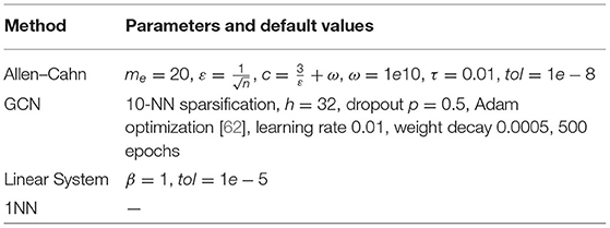
Table 2. Default parameters used in the experiments.

We split the presentation of the numerical results in the following way. We start by exploring the dependence of our schemes on some of the hyperparameters inherent in their derivation. We start by investigating the self-tuning parameters, namely the value of the chosen neighbor to compute the local scaling. We then study the performance of the Allen–Cahn model depending on the number of eigenpairs used for the approximation of the graph Laplacian. For our main study, we pair up all distance measures with all learning methods and report the results on all datasets. Furthermore, we investigate how the method's performance depends on the number of available training data using random training splits.

5.1. Self-Tuning Values

In section 2, we proposed the use of the self-tuning approach for the Gaussian function within the weight matrix. The crucial hyperparameter we want to explore now is the choice of neighbor k for the construction of σ_i = dist(x_i, x_k,i) with x_k,i the k-th nearest neighbor of the data point x_i. We can see from Table 3 that the small values k = 7, 20 perform quite well in comparison to the larger self-tuning parameters. As a result we will use these smaller values in all further computations.

TABLE 3

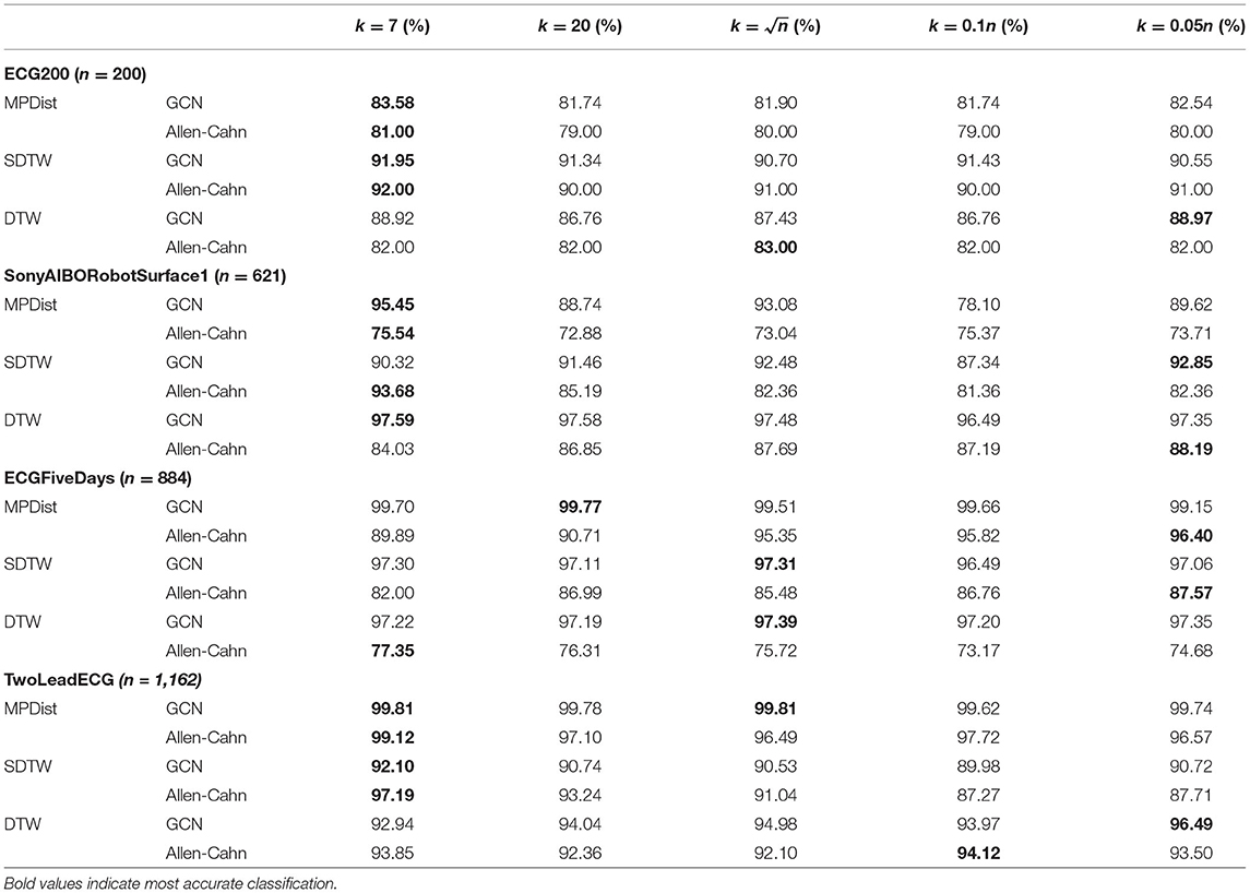
Table 3. Study of self-tuning parameters.

5.2. Spectral Approximation

As described in section 4 the Allen–Cahn equation is projected to a lower-dimensional space using the insightful information provided by the eigenvectors to the smallest eigenvalues of the graph Laplacian. We now investigate how the number of used eigenvectors impacts the accuracy. In the following we vary the number of eigenvalues from 10 to 190 and compare the performance of the Allen–Cahn method on three different datasets. The results are shown in Table 4 and it becomes clear that a vast number of eigenvectors does not lead to better classification accuracy. As a result we require a smaller number of eigenpair computations and also fewer computations within the Allen–Cahn scheme itself. The comparison was done for the self-tuning parameter k = 7.

TABLE 4

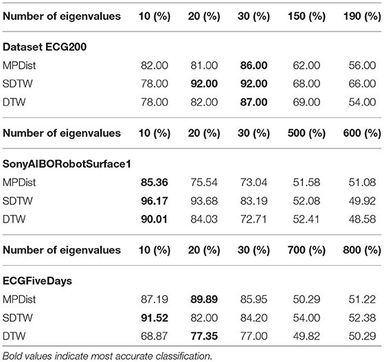
Table 4. Varying the number of eigenpairs for the reduced Allen–Cahn equation.

5.3. Full Method Comparison

We now compare the Allen-Cahn approach, the GCN scheme, the linear systems based method, and the 1NN algorithm, each paired up with each of the distance measures introduced in section 3. Full results are listed in Figures 6, 7. We show the comparison for all 42 datasets.

FIGURE 6

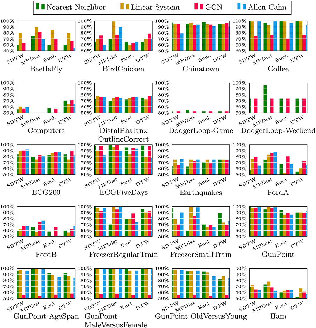
Figure 6. Comparison of the proposed methods using various distance measures for a variety of time series data. The size of the training set is specified in TwoClassProblems.csv within http://www.timeseriesclassification.com/Downloads/Archives/Univariate2018_arff.zip.

FIGURE 7

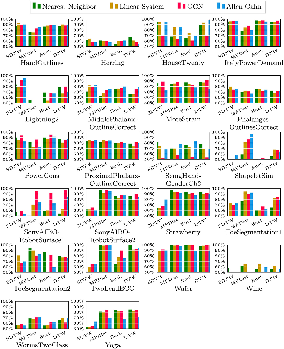
Figure 7. Comparison of the proposed methods using various distance measures for a variety of time series data.

As can be seen there are several datasets where the performance of all methods is fairly similar even when the distance measure is varied. Here, we name Chinatown, Earthquakes, GunPoint, ItalyPowerDemand, MoteStrain, Wafer. There are several examples where the methods do not seem to perform well, with GCN and 1NN relatively similar outperforming the Linear System and Allen–Cahn approach. Such examples are DodgerLoopGame, DodgerLoopWeekend. The GCN method clearly does not perform well with the GunPoint datasets where the other methods clearly perform well. It is surprising to note that the Euclidean distance, given its computational speed and simplicity, does not come out as underperforming with respect to the accuracy across the different methods. There are very few datasets where one distance clearly outperforms the other choice. We name ShapeletSim, ToeSegementation1 here. One might conjecture that the varying sizes of the training data might be a reason for the difference in performance of the models. To investigate this further we will next vary the training splits for all datasets and methods.

5.4. Varying Training Splits

In Figures 8–12, we vary the size of the training set from 1 to 20% of the available data. All reported numbers are averages over 100 random splits. The numbers we observe mirror the performance of the full training size. We see that the methods show reduced performance when only 1% of the training data are used but often reach an accuracy plateau when 5 to 10% of the training data are used. We observe that the size of the training set alone does not explain the different performance in the various datasets and methods applied here.

FIGURE 8

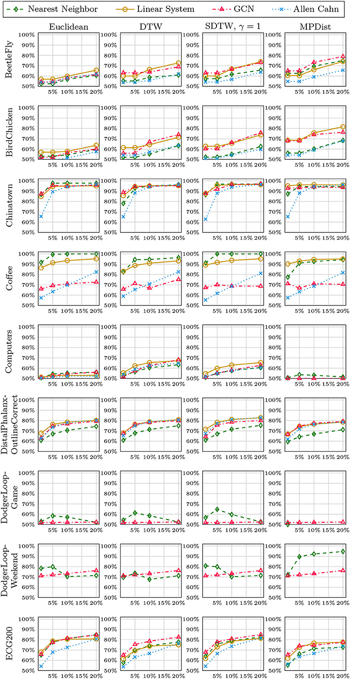
Figure 8. Method accuracy comparison for random training splits of different sizes (part 1/5).

FIGURE 9

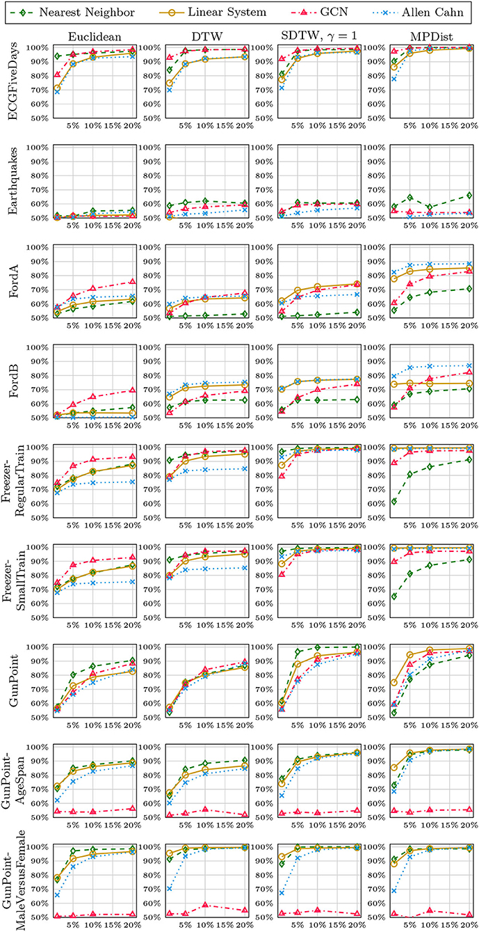
Figure 9. Method accuracy comparison for random training splits of different sizes (part 2/5).

FIGURE 10

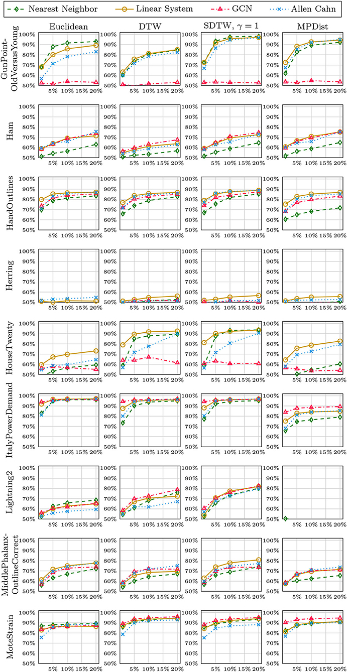
Figure 10. Method accuracy comparison for random training splits of different sizes (part 3/5).

FIGURE 11

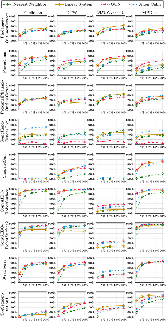
Figure 11. Method accuracy comparison for random training splits of different sizes (part 4/5).

FIGURE 12

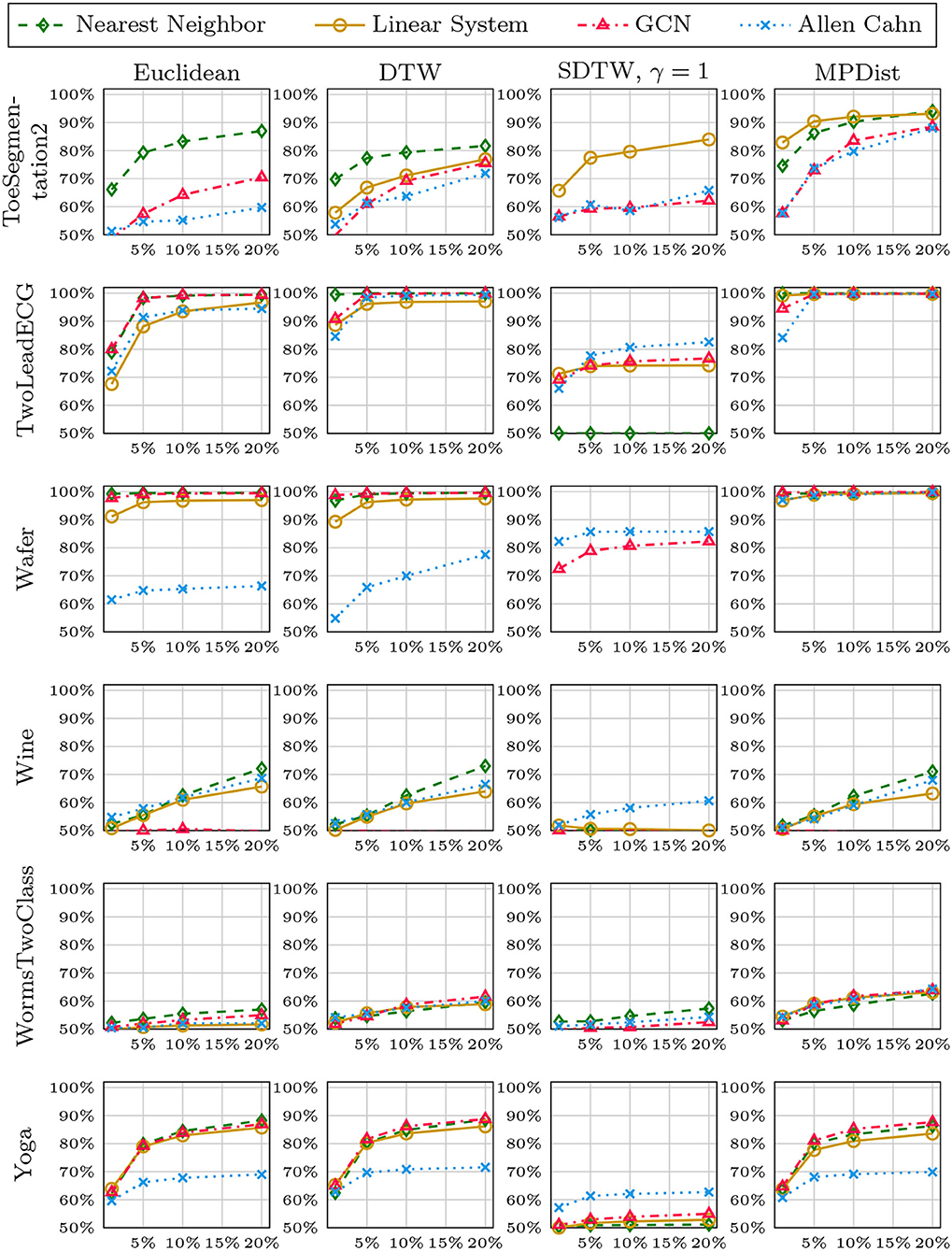
Figure 12. Method accuracy comparison for random training splits of different sizes (part 5/5).

6. Conclusion

In this paper we took to the task of classifying time series data in a semi-supervised learning setting. For this we proposed to represent the data as a fully-connected graph where the edge weights are created based on a Gaussian similarity measure (1). The heart of this function is the difference measure between the time series, for which we used the (Soft) Dynamic Time Warping and Matrix Profile based distance measures as well as the Euclidean distance. We then investigated several learning algorithms, namely, the Allen–Cahn-based method, the Graph Convolutional Network scheme, and a linear system approach, all reliant on the graph Laplacian, as well as the Nearest Neighbor method. We then illustrated the performance of all pairs of distance measure and learning methods. In this empirical study we observed that the methods tend to show an increased performance adding more training data. Studying all binary time-series with the timeseriesclassification.com repository gives results that in accordance with the no free lunch theorem show no clear winner. On the positive side the methods often perform quite well and there are only a few datasets with decreased performance. The comparison of the distance measures indicates there are certain cases where they outperform their competitors but also there is no clear winner with regards to accuracy. We believe that this empirical, reproducible study will encourage further research in this direction. Additionally, it might be interesting to consider model-based representations of time-series such as ARMA [63, 64] to use within the graph representations used here.

Data Availability Statement

The original contributions presented in the study are included in the article/supplementary material, further inquiries can be directed to the corresponding author/s.

Author Contributions

MG provide the initial implementation of some of the methods. MS supervised the other members, wrote parts of the manuscript, and implemented the Allen Cahn scheme. DB implemented the GCN approach, wrote parts of the manuscript, and oversaw the design of the tests. LP implemented several algorithms and wrote parts of the manuscript. All authors contributed to the article and approved the submitted version.

Funding

MS and LP acknowledge the funding of the BMBF grant 01|S20053A. DB was partially supported by KINTUC project [Sächsische Aufbaubank–Förderbank–(SAB) 100378180].

Conflict of Interest

The authors declare that the research was conducted in the absence of any commercial or financial relationships that could be construed as a potential conflict of interest.

Publisher's Note

All claims expressed in this article are solely those of the authors and do not necessarily represent those of their affiliated organizations, or those of the publisher, the editors and the reviewers. Any product that may be evaluated in this article, or claim that may be made by its manufacturer, is not guaranteed or endorsed by the publisher.

Acknowledgments

All authors would like to acknowledge the hard work and dedication by the team maintaining www.timeseriesclassification.com/. The publication of this article was funded by Chemnitz University of Technology.

Footnotes

1. ^We here view one time-series as a data point and the feature vector for this data point is the vector with the associated data collected in a vector.

2. ^Here the prototype of the cluster is the centroid.

3. ^This term is commonly used when the regression results shrink toward a mass at the barycenter of a target [44].

4. ^We focussed on all binary classification series listed in TwoClassProblems.csv within http://www.timeseriesclassification.com/Downloads/Archives/Univariate2018_arff.zip.

References

1. Fu TC. A review on time series data mining. Eng Appl Artif Intell. (2011) 24:164–81. doi: 10.1016/j.engappai.2010.09.007

CrossRef Full Text | Google Scholar

2. Bello-Orgaz G, Jung JJ, Camacho D. Social big data: recent achievements and new challenges. Inform Fusion. (2016) 28:45–59. doi: 10.1016/j.inffus.2015.08.005

PubMed Abstract | CrossRef Full Text | Google Scholar

3. Chen F, Deng P, Wan J, Zhang D, Vasilakos AV, Rong X. Data mining for the internet of things: literature review and challenges. Int J Distribut Sensor Netw. (2015) 11:431047. doi: 10.1155/2015/431047

PubMed Abstract | CrossRef Full Text | Google Scholar

4. Laptev N, Amizadeh S, Flint I. Generic and scalable framework for automated time-series anomaly detection. In: Proceedings of the 21th ACM SIGKDD International Conference on Knowledge Discovery and Data Mining. (2015). p. 1939–47. doi: 10.1145/2783258.2788611

CrossRef Full Text | Google Scholar

5. Chiu B, Keogh E, Lonardi S. Probabilistic discovery of time series motifs. In: Proceedings of the ninth ACM SIGKDD International Conference on Knowledge Discovery and Data Mining. (2003). p. 493–8. doi: 10.1145/956750.956808

CrossRef Full Text | Google Scholar

6. De Gooijer JG, Hyndman RJ. 25 years of time series forecasting. Int J Forecast (2006). 22:443–73. doi: 10.1016/j.ijforecast.2006.01.001

CrossRef Full Text | Google Scholar

7. Wei WW. Time series analysis. In: Todd little editor. The Oxford Handbook of Quantitative Methods in Psychology. Vol. 2. (2006).

Google Scholar

8. Chatfield C, Xing H. The Analysis of Time Series: An Introduction with R. CRC Press. (2019) doi: 10.1201/9781351259446

CrossRef Full Text | Google Scholar

9. Fawaz HI, Forestier G, Weber J, Idoumghar L, Muller PA. Deep learning for time series classification: a review. Data Mining Knowledge Discov. (2019) 33:917–63. doi: 10.1007/s10618-019-00619-1

CrossRef Full Text | Google Scholar

10. Abanda A, Mori U, Lozano JA. A review on distance based time series classification. Data Mining Knowledge Discov. (2019) 33:378–412. doi: 10.1007/s10618-018-0596-4

CrossRef Full Text | Google Scholar

11. Wei L, Keogh E. Semi-supervised time series classification. In: Proceedings of the 12th ACM SIGKDD International Conference on Knowledge Discovery and Data Mining. (2006). p. 748–53. doi: 10.1145/1150402.1150498

CrossRef Full Text | Google Scholar

12. Liao TW. Clustering of time series data-a survey. Pattern Recogn. (2005) 38:1857–74. doi: 10.1016/j.patcog.2005.01.025

PubMed Abstract | CrossRef Full Text | Google Scholar

13. Aghabozorgi S, Shirkhorshidi AS, Wah TY. Time-series clustering-a decade review. Inform Syst. (2015) 53:16–38. doi: 10.1016/j.is.2015.04.007

CrossRef Full Text | Google Scholar

14. Shifaz A, Pelletier C, Petitjean F, Webb GI. TS-CHIEF: a scalable and accurate forest algorithm for time series classification. Data Mining Knowledge Discov. (2020) 34:742–75. doi: 10.1007/s10618-020-00679-8

CrossRef Full Text | Google Scholar

15. Dempster A, Petitjean F, Webb GI. ROCKET: exceptionally fast and accurate time series classification using random convolutional kernels. Data Mining Knowledge Discov. (2020) 34:1454–95. doi: 10.1007/s10618-020-00701-z

CrossRef Full Text | Google Scholar

16. Fawaz HI, Lucas B, Forestier G, Pelletier C, Schmidt DF, Weber J, et al. Inceptiontime: Finding alexnet for time series classification. Data Mining Knowledge Discov. (2020) 34:1936–62. doi: 10.1007/s10618-020-00710-y

CrossRef Full Text | Google Scholar

17. Zhu X, Goldberg A. Introduction to Semi-supervised Learning. Morgan & Claypool Publishers (2009). doi: 10.2200/S00196ED1V01Y200906AIM006

CrossRef Full Text | Google Scholar

18. Chapelle O, Schölkopf B, Zien A. Semi-supervised learning. IEEE Trans Neural Netw. (2009) 20:542. doi: 10.1109/TNN.2009.2015974

PubMed Abstract | CrossRef Full Text | Google Scholar

19. Stoll M. A literature survey of matrix methods for data science. GAMM-Mitt. (2020) 43:e202000013:4. doi: 10.1002/gamm.202000013

PubMed Abstract | CrossRef Full Text | Google Scholar

20. Mercado P, Bosch J, Stoll M. Node classification for signed social networks using diffuse interface methods. In: ECMLPKDD. (2019). doi: 10.1007/978-3-030-46150-8_31

CrossRef Full Text | Google Scholar

21. Kipf TN, Welling M. Semi-supervised classification with graph convolutional networks. arXiv [Preprint]. arXiv:160902907 (2016).

PubMed Abstract | Google Scholar

22. Bertozzi AL, Luo X, Stuart AM, Zygalakis KC. Uncertainty quantification in graph-based classification of high dimensional data. SIAM/ASA J Uncertainty Quant. (2018) 6:568–95. doi: 10.1137/17M1134214

CrossRef Full Text | Google Scholar

23. von Luxburg U. A tutorial on spectral clustering. Stat Comput. (2007) 17:395–416. doi: 10.1007/s11222-007-9033-z

PubMed Abstract | CrossRef Full Text | Google Scholar

24. Bruna J, Zaremba W, Szlam A, LeCun Y. Spectral networks and locally connected networks on graphs. arXiv [Preprint]. arXiv:13126203 (2013).

Google Scholar

25. Chung FR, Graham FC. Spectral graph Theory. American Mathematical Soc. (1997).

Google Scholar

26. Jung A. Networked exponential families for big data over networks. IEEE Access. (2020) 8:202897–909. doi: 10.1109/ACCESS.2020.3033817

PubMed Abstract | CrossRef Full Text | Google Scholar

27. Jung A, Tran N. Localized linear regression in networked data. IEEE Signal Process Lett. (2019) 26:1090–4. doi: 10.1109/LSP.2019.2918933

PubMed Abstract | CrossRef Full Text | Google Scholar

28. Müller M. Information Retrieval for Music and Motion. vol. 2. Springer (2007). doi: 10.1007/978-3-540-74048-3

CrossRef Full Text | Google Scholar

29. Cuturi M, Blondel M. Soft-DTW: a differentiable loss function for time-series. In: International Conference on Machine Learning. PMLR (2017). p. 894–903.

Google Scholar

30. Gharghabi S, Imani S, Bagnall A, Darvishzadeh A, Keogh E. An ultra-fast time series distance measure to allow data mining in more complex real-world deployments. Data Mining Knowledge Discov. (2020) 34:1104–35. doi: 10.1007/s10618-020-00695-8

CrossRef Full Text | Google Scholar

31. Bertozzi AL, Flenner A. Diffuse interface models on graphs for classification of high dimensional data. Multiscale Model Simul. (2012) 10:1090–118. doi: 10.1137/11083109X

CrossRef Full Text | Google Scholar

32. Bagnall A, Lines J, Bostrom A, Large J, Keogh E. The great time series classification bake off: a review and experimental evaluation of recent algorithmic advances. Data mining Knowledge Discov. (2017) 31:606–60. doi: 10.1007/s10618-016-0483-9

PubMed Abstract | CrossRef Full Text | Google Scholar

33. Ruiz AP, Flynn M, Large J, Middlehurst M, Bagnall A. The great multivariate time series classification bake off: a review and experimental evaluation of recent algorithmic advances. Data Mining Knowledge Discov. (2021) 35:401–49. doi: 10.1007/s10618-020-00727-3

PubMed Abstract | CrossRef Full Text | Google Scholar

34. MacQueen J. Some methods for classification and analysis of multivariate observations. In: Proceedings of the Fifth Berkeley Symposium on Mathematical Statistics and Probability. Oakland, CA (1967). p. 281–97.

PubMed Abstract | Google Scholar

35. MacKay DJ, Mac Kay DJ. Information Theory, Inference and Learning Algorithms. Cambridge University Press (2003).

Google Scholar

36. Belkin M, Niyogi P. Laplacian eigenmaps and spectral techniques for embedding and clustering. In: Advances in Neural Information Processing Systems. (2001). p. 585–91.

PubMed Abstract | Google Scholar

37. Shawe-Taylor J, Cristianini N. Kernel Methods for Pattern Analysis. Cambridge University Press (2004). doi: 10.1017/CBO9780511809682

PubMed Abstract | CrossRef Full Text | Google Scholar

38. Hofmann T, Schölkopf B, Smola AJ. Kernel methods in machine learning. Ann Stat. (2008) 36:1171–220. doi: 10.1214/009053607000000677

PubMed Abstract | CrossRef Full Text | Google Scholar

39. Zelnik-Manor L, Perona P. Self-tuning spectral clustering. In: Advances in Neural Information Processing Systems. (2005). p. 1601–8.

Google Scholar

40. Keogh E, Kasetty S. On the need for time series data mining benchmarks: a survey and empirical demonstration. Data Mining Knowledge Discov. (2003) 7:349–71. doi: 10.1023/A:1024988512476

CrossRef Full Text | Google Scholar

41. Salvador S, Chan PK. Toward accurate dynamic time warping in linear time and space. Intell Data Anal. (2004) 11:70–80. doi: 10.3233/IDA-2007-11508

CrossRef Full Text | Google Scholar

42. Wu R, Keogh EJ. FastDTW is approximate and generally slower than the algorithm it approximates. IEEE Trans Knowledge Data Eng. (2020). doi: 10.1109/TKDE.2020.3033752

PubMed Abstract | CrossRef Full Text | Google Scholar

43. Blondel M, Mensch A, Vert JP. Differentiable divergences between time series. arXiv [Preprint]. arXiv:201008354 (2020).

Google Scholar

44. Lin H, Hong X, Ma Z, Wei X, Qiu Y, Wang Y, et al. Direct measure matching for crowd counting. arXiv [Preprint]. arXiv:210701558 (2021). doi: 10.24963/ijcai.2021/116

CrossRef Full Text | Google Scholar

45. Taylor JE, Cahn JW. Linking anisotropic sharp and diffuse surface motion laws via gradient flows. J Statist Phys. (1994) 77:183–97. doi: 10.1007/BF02186838

CrossRef Full Text | Google Scholar

46. Allen SM, Cahn JW. A microscopic theory for antiphase boundary motion and its application to antiphase domain coarsening. Acta Metall. (1979) 27:1085–95. doi: 10.1016/0001-6160(79)90196-2

CrossRef Full Text | Google Scholar

47. Cahn JW, Hilliard JE. Free energy of a nonuniform system. I. Interfacial free energy. J Chem Phys. (1958) 28:258–67. doi: 10.1063/1.1744102

PubMed Abstract | CrossRef Full Text | Google Scholar

48. Bosch J, Kay D, Stoll M, Wathen A. Fast solvers for Cahn-Hilliard inpainting. SIAM J Imaging Sci. (2014) 7:67–97. doi: 10.1137/130921842

CrossRef Full Text | Google Scholar

49. Bertozzi AL, Esedoglu S, Gillette A. Inpainting of binary images using the Cahn-Hilliard equation. IEEE Trans Image Process. (2007) 16:285–91. doi: 10.1109/TIP.2006.887728

PubMed Abstract | CrossRef Full Text | Google Scholar

50. Garcia-Cardona C, Merkurjev E, Bertozzi AL, Flenner A, Percus AG. Multiclass data segmentation using diffuse interface methods on graphs. IEEE Trans Pattern Anal Mach Intell. (2014) 36:1600–13. doi: 10.1109/TPAMI.2014.2300478

PubMed Abstract | CrossRef Full Text | Google Scholar

51. Bosch J, Klamt S, Stoll M. Generalizing diffuse interface methods on graphs: nonsmooth potentials and hypergraphs. SIAM J Appl Math. (2018) 78:1350–77. doi: 10.1137/17M1117835

CrossRef Full Text | Google Scholar

52. Bergermann K, Stoll M, Volkmer T. Semi-supervised learning for multilayer graphs using diffuse interface methods and fast matrix vector products. SIAM J Math Data Sci. (2021). doi: 10.1137/20M1352028

CrossRef Full Text | Google Scholar

53. Budd J, van Gennip Y. Graph MBO as a semi-discrete implicit Euler scheme for graph Allen-Cahn. arXiv [Preprint]. arXiv:190710774 (2019). doi: 10.1137/19M1277394

CrossRef Full Text | Google Scholar

54. Budd J, van Gennip Y, Latz J. Classification and image processing with a semi-discrete scheme for fidelity forced Allen-Cahn on graphs. arXiv [Preprint]. arXiv:201014556 (2020). doi: 10.1002/gamm.202100004

PubMed Abstract | CrossRef Full Text | Google Scholar

55. Calatroni L, van Gennip Y, Schönlieb CB, Rowland HM, Flenner A. Graph clustering, variational image segmentation methods and Hough transform scale detection for object measurement in images. J Math Imaging Vision. (2017) 57:269–91. doi: 10.1007/s10851-016-0678-0

CrossRef Full Text | Google Scholar

56. Goodfellow I, Bengio Y, Courville A, Bengio Y. Deep Learning. vol. 1. Cambridge: MIT Press (2016).

Google Scholar

57. LeCun Y, Bengio Y, Hinton G. Deep learning. Nature. (2015) 521:436–44. doi: 10.1038/nature14539

PubMed Abstract | CrossRef Full Text | Google Scholar

58. Zhang S, Tong H, Xu J, Maciejewski R. Graph convolutional networks: a comprehensive review. Comput Soc Netw. (2019) 6:1–23. doi: 10.1186/s40649-019-0069-y

CrossRef Full Text | Google Scholar

59. Alfke D, Stoll M. Pseudoinverse graph convolutional networks: fast filters tailored for large eigengaps of dense graphs and hypergraphs. Data Mining Knowledge Discov. (2021). doi: 10.1007/s10618-021-00752-w

CrossRef Full Text | Google Scholar

60. Xu Z, Funaya K. Time series analysis with graph-based semi-supervised learning. In: 2015 IEEE International Conference on Data Science and Advanced Analytics (DSAA). IEEE (2015). p. 1–6. doi: 10.1109/DSAA.2015.7344902

PubMed Abstract | CrossRef Full Text | Google Scholar

61. Dau HA, Bagnall A, Kamgar K, Yeh CCM, Zhu Y, Gharghabi S, et al. The UCR time series archive. IEEE/CAA J Automat Sin. (2019) 6:1293–305. doi: 10.1109/JAS.2019.1911747

PubMed Abstract | CrossRef Full Text | Google Scholar

62. Kingma D, Ba JL. Adam: a method for stochastic optimization. In: Proc Int Conf Learn Represent. ICLR'15. (2015).

Google Scholar

63. Brockwell PJ, Davis RA. Time Series: Theory and Methods. Springer Science & Business Media (2009).

Google Scholar

64. Spiegel S. Time series distance measures. Ph.D. thesis. Berlin, Germany.

Google Scholar