Modeling of COVID-19 Pandemic vis-à-vis Some Socio-Economic Factors

1 Introduction

Modeling of COVID-19 by scientists, epidemiologists, and health experts was considered early on in the pandemic as it began to ravage the world. The socio-economic determinants of this pandemic taken into account in this modeling are important because they condition the severity of an affected country and the way in which it is controlled, which leads to consider the corresponding variables alongside the daily reproduction rates during the period of contagiousness of individuals infected by the pandemic. The aim of this article is to show the joint variations of socio-economic determinants and epidemiological parameters, which can be observed between developed and developing states and between successive epidemic waves.

Some researchers have already worked on socio-economic analysis of the COVID-19 pandemic: in [1], the authors examined the geoclimatic, demographic, and socio-economic determinants of COVID-19 prevalence and have shown that the influence of these determinants varies by comparing the first and second wave of the pandemic. The socio-economic impact of the COVID-19 pandemic in United States of America (United States) was studied by Barlow and Vodenska [2], where the authors investigate the systematic risk posted by sector-level industries within the United States. Ahmed et al. [3] modeled daily confirmed cases of COVID-19 in different countries across the globe using regression models with predictions for upcoming scenarios. Kong et al. [4] worked on the socio-economic and environmental factors influencing the basic reproduction number of the COVID-19 pandemic by fitting a logistic growth curve to the reported daily cases up to the first peak of the pandemic while Qiu et al. [5] studied the impact of socio-economic factors on the transmission of COVID-19 disease with China as a case study using an empirical model, and the authors conclude that these determinants have rich implications for ongoing efforts in containing the pandemic. The work in this present article is an extension of [6], which was based on the analysis of the reproduction numbers of COVID-19 based on the Current Health Expenditure as Gross Domestic Product Percentage (CHE/GDP) across several countries using some machine learning tools. The results of this study show that some countries with a high CHE/GDP improved their public health strategy against the virus during the second wave of the pandemic, fighting it all the more effectively against it the more effectively they were. the most affected during the first wave. The difference with the present study lies in the fact that the latter takes into account data from twice as many public sites [7–17] and that it is more focused on social inequality, quantified for example by the Social Fracture coefficient (SF equal to the ratio between the incomes of the richest 10% and the poorest 10% of a given population), and the Theil and Gini indices. It was shown previously in [18] that the Gini index was highly correlated (r = 0.93) to another Demo-economic index denoted DI and equal to the quotient (CHE/GDP)/SF, proving that all these indices are closely related and carry part of the causality of inter-country variations in epidemiological parameters.

The main objectives of this article are to establish a relationship between Theil and Gini index, analyze critically some of the socio-economic determinants of the pandemic, correlate them, predict three of the socio-economic variables, and perform some regression analyses. We have also clustered countries according to these parameters with the help of the lasso (least absolute shrinkage and selection operator) method, and we were able to select the best variables for the COVID-19 modeling.

The paper is divided into seven sections: after an introductive section, we explain in Section 2 the methodology used in this research, Section 3 deals with the variables used, Section 4 establishes a mathematical relationship between Theil and Gini index, Section 5 is dedicated to the visualization of the results obtained, while we finally give the discussion and conclusion in Sections 6 and 7, respectively.

2 Methods

The use of machine learning methods to analyze data has been helpful over the years to get a proper view on how a model behaves. In this research, we used some supervised and unsupervised machine learning methods and we also tried to use one deep learning method for the identification and visualization of clusters. To jointly interpret the socio-economic and epidemiological data, we have chosen these three main classes of the descriptive statistics, which allow us to compare these socio-economic and epidemiological data. Supervised learning is used in its regression function (prediction of a quantitative variable from annotated examples) and unsupervised learning (in which the data is not labeled) in its classification function. As for deep learning, it makes it possible to create a model from large-scale unlabeled data.

The supervised machine learning methods we used are first univariate polynomial regression, linear regression, lasso regression, and ridge regression. We also use some of these methods to make prediction by training the model and testing some percentage of the values. Lasso regression helped us to know the best variables to be used in the modeling. After the univariate regressions, we introduced multivariate least square methods, allowing us to test much more complex relations between variables. It can be represented as follows:

$\begin{array}{l}\mathit{y}={\mathbf{\beta }}_1{\mathbf{x}}_1+{\mathbf{\beta }}_2{\mathbf{x}}_2+\cdots +\in ,\end{array}(1)$

Where ${\mathbf{\beta }}_1,{\mathbf{\beta }}_2,\cdots$ are coefficients or weights, $\in$ is the residual noise, y is the dependent variable, and ${\mathbf{x}}_1,{\mathbf{x}}_2,\cdots$ are the independent variables. Ridge and lasso regression are simple methods to reduce the model complexity and prevent over-fitting, which may result from linear regression. The cost function for ridge regression is given below:

${\displaystyle {\sum }_{\mathit{i}=1}^{\mathit{n}}{\left({\mathit{y}}_{\mathit{i}}-{\widehat{\mathit{y}}}_{\mathit{i}}\right)}^2}={\displaystyle {\sum }_{\mathit{i}=1}^{\mathit{n}}{\left({\mathit{y}}_{\mathit{i}}-{\displaystyle {\sum }_{\mathit{j}=0}^{\mathit{m}}{\mathbf{\beta }}_{\mathit{j}}\times {\mathit{x}}_{\mathit{ij}}}\right)}^2}+\mathit{\alpha }{\displaystyle {\sum }_{\mathit{j}=0}^{\mathit{m}}{\mathbf{\beta }}_{\mathit{j}}^2}(2)$

with for some c > 0, ${\displaystyle {\sum }_{\mathit{j}=0}^{\mathit{m}}{\mathbf{\beta }}_{\mathit{j}}^2<\mathit{c}}$, while $\mathit{\alpha }$ is the penalty term that regularizes the coefficients such that if the coefficients take large values, the optimization function is penalized. Ridge regression puts constraint on the coefficients $\mathbf{\beta }$. We define the cost function for lasso regression in the same way, but by replacing the L2 penalty term by an L1 one as:

${\displaystyle {\sum }_{\mathit{i}=1}^{\mathit{n}}{\left({\mathit{y}}_{\mathit{i}}-{\widehat{\mathit{y}}}_{\mathit{i}}\right)}^2}={{\displaystyle {\sum }_{\mathit{i}=1}^{\mathit{n}}\left({\mathit{y}}_{\mathit{i}}-{\displaystyle {\sum }_{\mathit{j}=0}^{\mathit{m}}{\mathbf{\beta }}_{\mathit{j}}\times {\mathit{x}}_{\mathit{ij}}}\right)}}^2+\mathit{\alpha }{\displaystyle {\sum }_{\mathit{j}=0}^{\mathit{m}}\left|{\mathbf{\beta }}_{\mathit{j}}\right|}(3)$

with for some c > 0, ${\displaystyle {\sum }_{\mathit{j}=0}^{\mathit{m}}\left|{\mathbf{\beta }}_{\mathit{j}}\right|<\mathit{c}}$.

After the supervised learning methods, we used unsupervised learning approches to cluster variables across countries and the methods we proposed to validate our results were K-means clustering, Hierarchy clustering, and Principal Component Analysis (PCA). We also performed correlation calculations among parameters used in the modeling step and we chose an optimization method called Ordinary Least Square (OLS) for the socio-economic determinants of COVID-19. Eventually, the deep learning methods we used were Neural Network (NN) and Multi-Layer Perceptron (MLP) regressor, which is a class of feedforward Artificial Neural Network (ANN).

3 Variables

3.1 Socio-Economic Variables

Socio-economic variables constitute a strong determinant of the spread of the pandemic. We extracted some observed socio-economic variables from [7–17], while we also calculated other socio-economic variables like the socio-economic fracture index F, equal to the quotient between CHR/GDP and SF.

The observed variables used in this research are immigration rate (IR), average life expectancy (LE), Tuberculosis incidence (TB), temperature, percentage of gross domestic product devoted to health expenditure (CHE/GDP) collated from [16], percentage of 10% lowest (LI) and 10% highest incomes (HI), government response stringency index (SI), sustainable development goal (SDG) index, human development index (HDI), environmental performance index (EPI), consumer confidence index (CCI), stringency index (SI), Theil index (TI), and Gini index (GI). We collated the data on the available countries and most recent years in public databases [7–17].

The calculated socio-economic variables are as follows:

- Social fracture (SF) index is the ratio between the 10% highest income and the 10% lowest income. In brief, it is expressed by the equation below:

$\mathit{SF}=\frac{10\%\mathit{HI}}{10\%\mathit{LI}}(4)$

- Demo-economic (DI) index is the ratio between the percentage of GDP devoted to health expenditure and social fracture index. It is expressed by the equation below:

$DI=\frac{CHE/GDP}{SF}(5)$

We give a precise value of all variables in Table 1 and in Supplementary Table S2–S5 in the supplementary material.

TABLE 1

TABLE 1. Comparison of different regression models for the prediction.

3.2 Epidemiologic Variables

We have six epidemiologic variables: first wave maximum $R_o$, second wave maximum $R_o$, first wave deterministic $R_o$, second wave deterministic $R_o$, and opposite of the initial autocorrelation slope averaged on 6 days for both first and second wave of the daily new cases for developed and developing countries. All epidemiologic variables values were taken from [18] (see also the Appendix in [6]).

The epidemiologic variables were recorded during the exponential phase of the first and second wave of the pandemic. Daily new cases observed during the first 100 days were used to calculate the exponential slope for the first and second wave. The opposite of the initial autocorrelation slope was averaged on 6 days for the first and second wave. The maximum $R_o$ was collated from [6] while observing this value during the first and second waves of countries considered. We also collated from [6] the deterministic $R_o$ for the first and second wave of the pandemic taking 6 days as length of contagiousness period.

In this present study, we validated our results by performing cross-validation and also training 80% of the data and training 30%.

4 The Relationship Between Theil Index and Gini Index

4.1 Mathematical Approach

We first show the relationship between Theil index and Gini index mathematically. The Gini index is defined as follows [16]:

$\text{GI}=1-{\displaystyle \sum _{\text{k}=1,\text{n}}\left(\text{Xk}-\text{Xk}-1\right)\left(\text{yk}-\text{yk}-1\right)}=1-\text{E}\left(\Delta \right)=\text{E}\left(1-\Delta \right),(6)$

where x_k (respectively y_k) denotes the kth cumulative part of the population (respectively income). If we choose the population increments, d_k = x_k-x_k-1 are equal to 1/n, and if E(Δ) represents the expectation of the increment, Δ_k = y_k−y_k−1 for the distribution d_k. Then, the Theil index applied to the percentage y_k of the total income relative to a percentage x_k of the total population ([17]) is defined by the following equation:

$\text{TI}=-{\displaystyle \sum _{\text{k}=1,\text{n}}\left({\text{y}}_{\text{k}}-{\text{y}}_{\text{k}}-1\right)}\text{Log}\left({\text{y}}_{\text{k}}-{\text{y}}_{\text{k}}-1\right)=-{\displaystyle \sum _{\text{k}=1,\text{n}}\Delta \text{kLog}\left(\Delta \text{k}\right)}(7)$

If the first increment of y, Δ₁ = y₁ ≤ 1, is close to 1 [which corresponds to a square-shaped Lorenz curve, i.e., closed to a left right triangle-shaped income vs. population curve (in red on Figure 1), or to a high Gini index close to 1], then we have: ₋Log(Δ₁) ∼ 1₋Δ₁ and Δ_k ∼ 0, for k > 1. Then, we get:

$\text{TI}\sim -\text{Log}\left({\Delta }_1\right)\sim 1-{\Delta }_1\sim \text{GI},(8)$

the equality being available only if the Lorenz curve presents a perfect left right triangle shape.

FIGURE 1

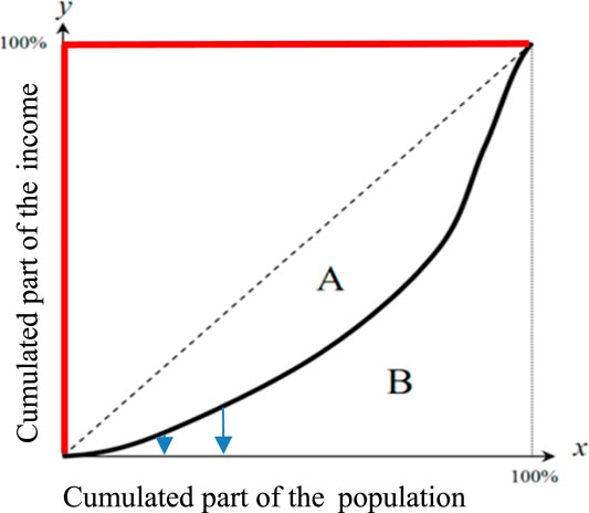
FIGURE 1. Lorenz curve showing the cumulated part of income vs. cumulated part of a population having this cumulated income. The curve in red represents left right triangle-shaped Lorenz curve.

4.2 Statistical Approach and Application to Latino-American Countries

4.2.1 Correlation

We correlated both Theil and Gini indices with all epidemiologic, demographic, and socio-economic variables, and as it can be seen in Figure 2G, Theil and Gini indices are highly positively correlated with coefficient 0.7.

FIGURE 2

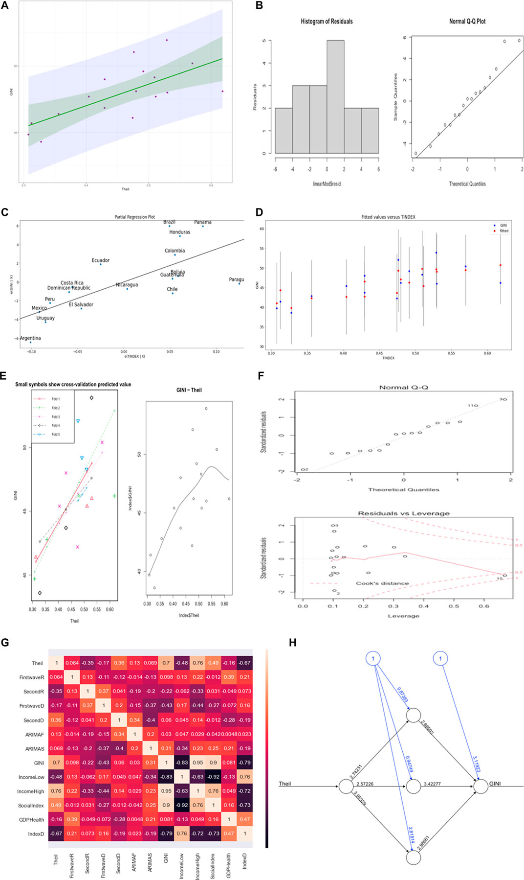
FIGURE 2. (A) Linear regression line (in green) with the confidence interval (in gray). (B) Residual plot for the linear regression. (C) Partial regression plot. (D) Fit plot. (E) On left-hand side is the cross-validation plot for the linear regression and on right-hand side is the polynomial regression plot. (F) Residual plots for polynomial regression. (G) Heat map for the correlations between all variables. (H) Neural network visualization.

4.2.2 Neural Network for Theil Index and Gini Index

We used the neuralnet package in R in order to visualize the weights of the network and the bias between Theil and Gini index, and as it can be seen in Figure 2H, the weights are good with low bias.

4.2.3 Regression Analysis Between Theil Index and Gini Index

Linear regression models use some historic data concerning independent and dependent variables and consider a linear relationship between both while polynomial regression models use a similar approach but the dependent variable is modeled as a degree m (m = 2 in the present study) polynomial in x.

Linear regression model is given as:

$\text{y}={\mathbf{\beta }}_{\mathbf{o}}+{\displaystyle \sum _{i=1,n}{\mathbf{\beta }}_{\mathbf{i}}{\mathbf{x}}_{\mathbf{i}}+{\in }_{\mathit{i}},}(9)$

where ${\mathbf{\beta }}_{\mathbf{i}}\mathit{\text{'}s}$ are the weights, ${\mathbf{\beta }}_{\mathbf{o}}$ is the intercept and $\in$ is the random error term. The above equation is the linear equation that needs to be obtained with the minimum error. Polynomial regression of order 2 is given below:

$\text{y}={\mathbf{\beta }}_{\mathbf{o}}+{\mathbf{\beta }}_{\mathbf{i}}{\text{x}}_1+{\displaystyle \sum _{i=1,n}{\mathbf{\beta }}_{\mathbf{i}}{\mathit{x}}_{\mathit{i}}^2+{\in }_{\mathit{i}}},(10)$

We present the visualization of the regression results using this approach in Figures 2A–F.

For the linear regression as shown in Figure 2A, the intercept is 31.03, p-value is 0.0181, R² is 0.4881, residual standard error is 3.116, and all coefficients are significant with p < 0.05 for both the train and test data for linear and polynomial regression. The median of the residual plot in Figures 2B,F are 0.2111 and 0.2566, respectively, for both linear and polynomial regression, which are low values. The normality of the residual was tested using Jarque-Bera and Durbin-Watson tests, which gave a high p-value, and we failed to reject the null hypothesis that the skewness and kurtosis of the residuals are statistically equal to zero. In order to know the performance of the linear regression model, we trained 80% of the data and tested the 20% remaining data and also did cross-validation to be sure of the accuracy. The predicted and the observed values are very close to the results presented for the regression models used. For the linear model, we present the cross-validation result in Figure 2E whose average mean square error for the five portion folds is 11.72794. We observed that the correlation between the tested and the predicted values has high accuracy (R² = 0.97). The test set p-value is 0.02 with a residual standard error of 3.528. For polynomial regression of order 2, the train set has the following results: R² = 0.6, p-value = 0.002, and residual standard error = 2.935. The test set has the following results: R² = 0.99, p-value = 0.008, and residual standard error = 0.5639.

4.2.4 Multivariate Analysis for Gini Index and Theil Index Alongside Other Socio-Economic Variables and Epidemiologic Variables

Figure 3 corresponds to the ordinary multivariate least square methods with R² = 0.674. Figure 3A shows Paraguay as outlier not fitting data, Figure 3B normalizes all countries and does not point any country in the plot.

FIGURE 3

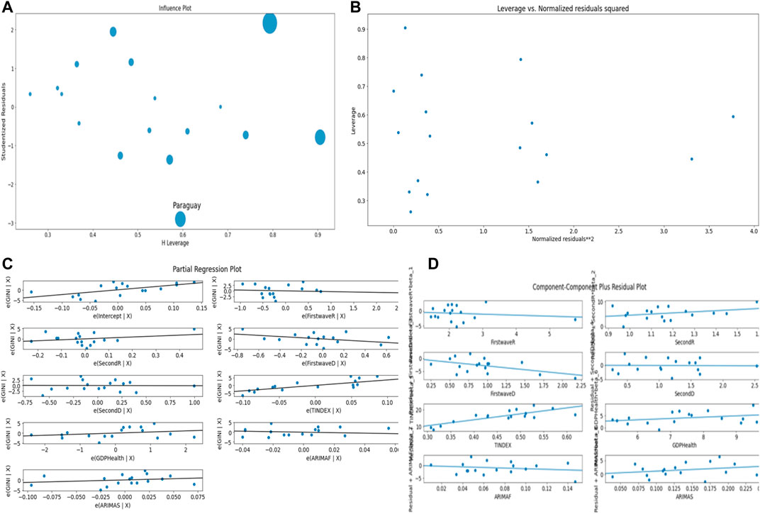
FIGURE 3. (A) Influence plot. (B) Leverage vs. Normalized residuals squared plot. (C) Partial regression plot. (D) Component–Component plus residual plot.

4.2.5 Prediction of Gini Index Using MLP Regressor, and Linear, Lasso, and Ridge Regression

In this section, we used cross-validation method to choose the best parameter $\alpha$ for the modeling as shown in Figure 4C. For ridge regression, $\alpha =0.142$ with a mean square error of 1.36 and $\alpha =0.368$ for lasso regression with a mean square error = 5.10. For Figure 4E, training score = 1.000 and test score = 0.641; for Figure 4F, training score = 0.992 and test score = 0.497; for Figure 4G, training score = 0.99 and test score = 0.406; and for Figure 4H, training score = 0.984 and test score = −0.077. It is evident from these results that linear regression best predicts Gini index with the highest test score, and predicted values are very close to each other as presented in Table 1. Also, we observed the same pattern of prediction in Figures 4E–H showing that all methods used in this section have the same predictive behavior.

FIGURE 4

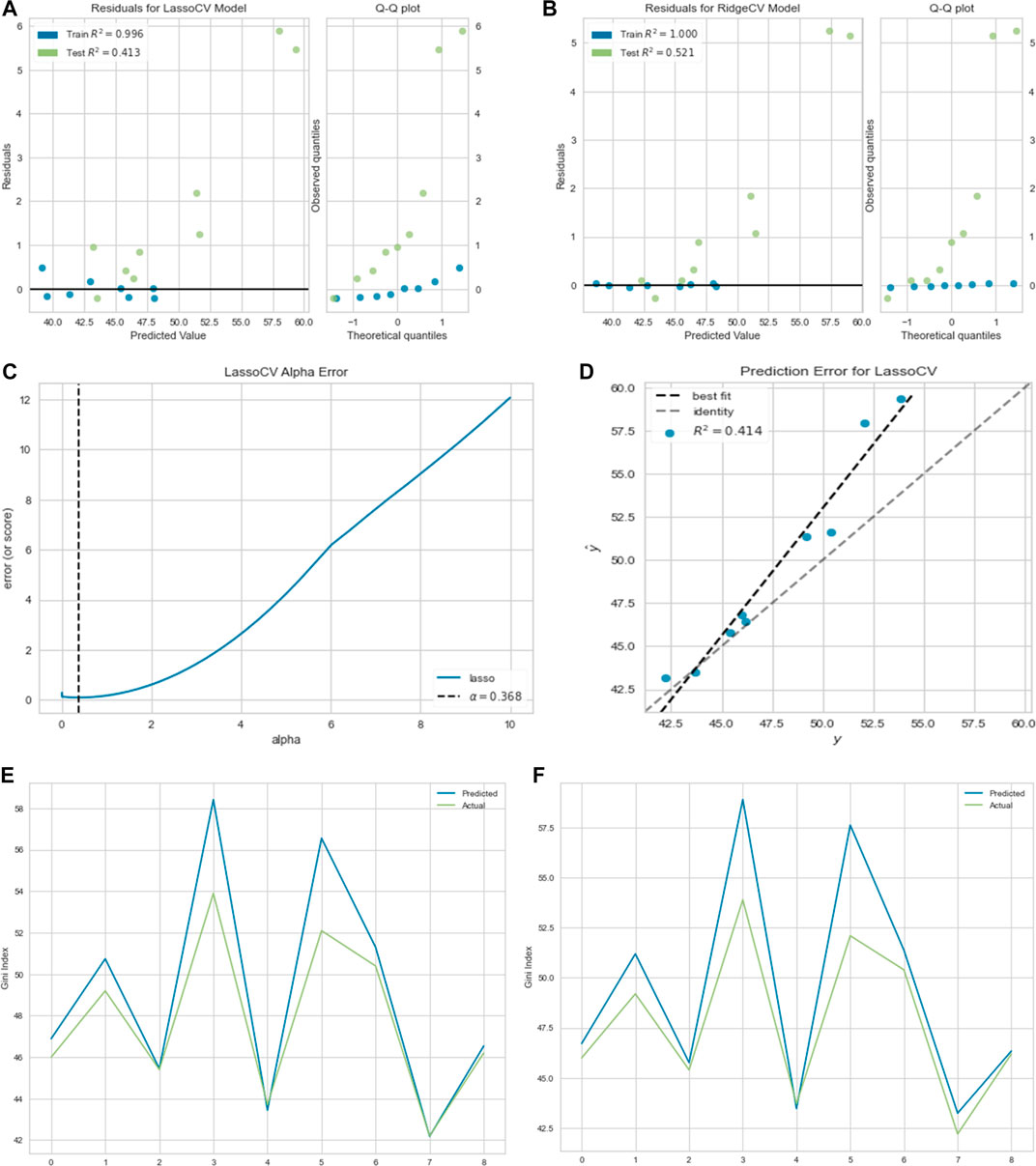
FIGURE 4. (A) Residual plot for lasso regression. (B) Residual plot for ridge regression. (C) Lasso regression cross-validation error. (D) Prediction error for the lasso regression. (E) Linear regression prediction plot. (F) Lasso regression and (G) ridge regression prediction plots. (H) MLP regression prediction plot.

4.2.6 Clustering Analysis of Latino-American Countries for Gini Index and Theil Index Alongside Other Socio-Economic Variables and Epidemiologic Variables

In Figure 5C, the first two clusters have 14 countries and the third has three countries, which are Uruguay and El Salvador on the same hierarchy while Argentina is on another hierarchy. We only show the cluster dendrogram for the first cluster. In Figure 5F, the Gini index has the highest positive correlation of 0.44 with the principal component PC 1 and Theil index has only the value 0.34 with PC 1. The main variable causing the separation into three classes is the Gini index.

FIGURE 5

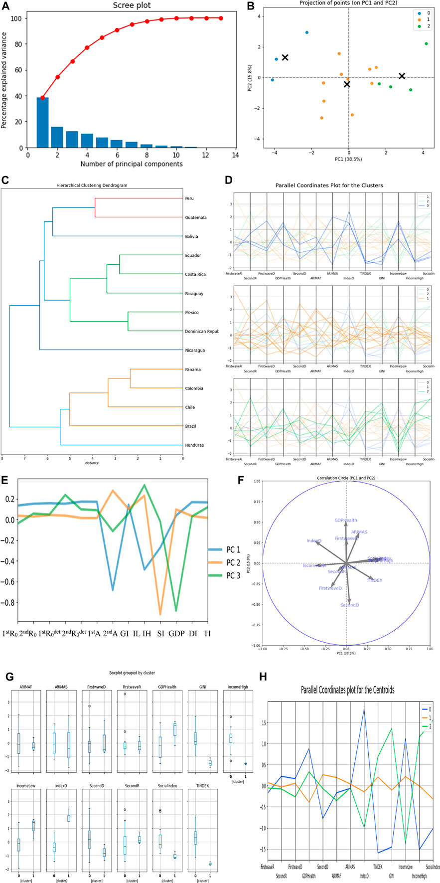
FIGURE 5. (A) Scree plot. (B) Plot for projection of points for PC1 and PC2. (C) Hierarchy clustering dendrogram. (D) Parallel coordinates plot for the clusters. (E,F) PC’s visualization. (G) Box plot for the clusters. (H) Parallel coordinates plot for the centroids.

5 Application of the Methods to OECD Countries, African Countries, and Developed and Developing Countries

5.1 Developed and Developing Countries

5.1.1 Regression and Multivariate Analysis for Socio-Economic and Epidemiologic Variables

In Figures 6C,D, we modeled the dependent variable as a degree n (n = 6 in the present study) polynomial in x, an extension of Eq. 8. Figure 6 presents regression analyses with the parameters presented in Supplementary Table S6 in the supplementary material.

FIGURE 6

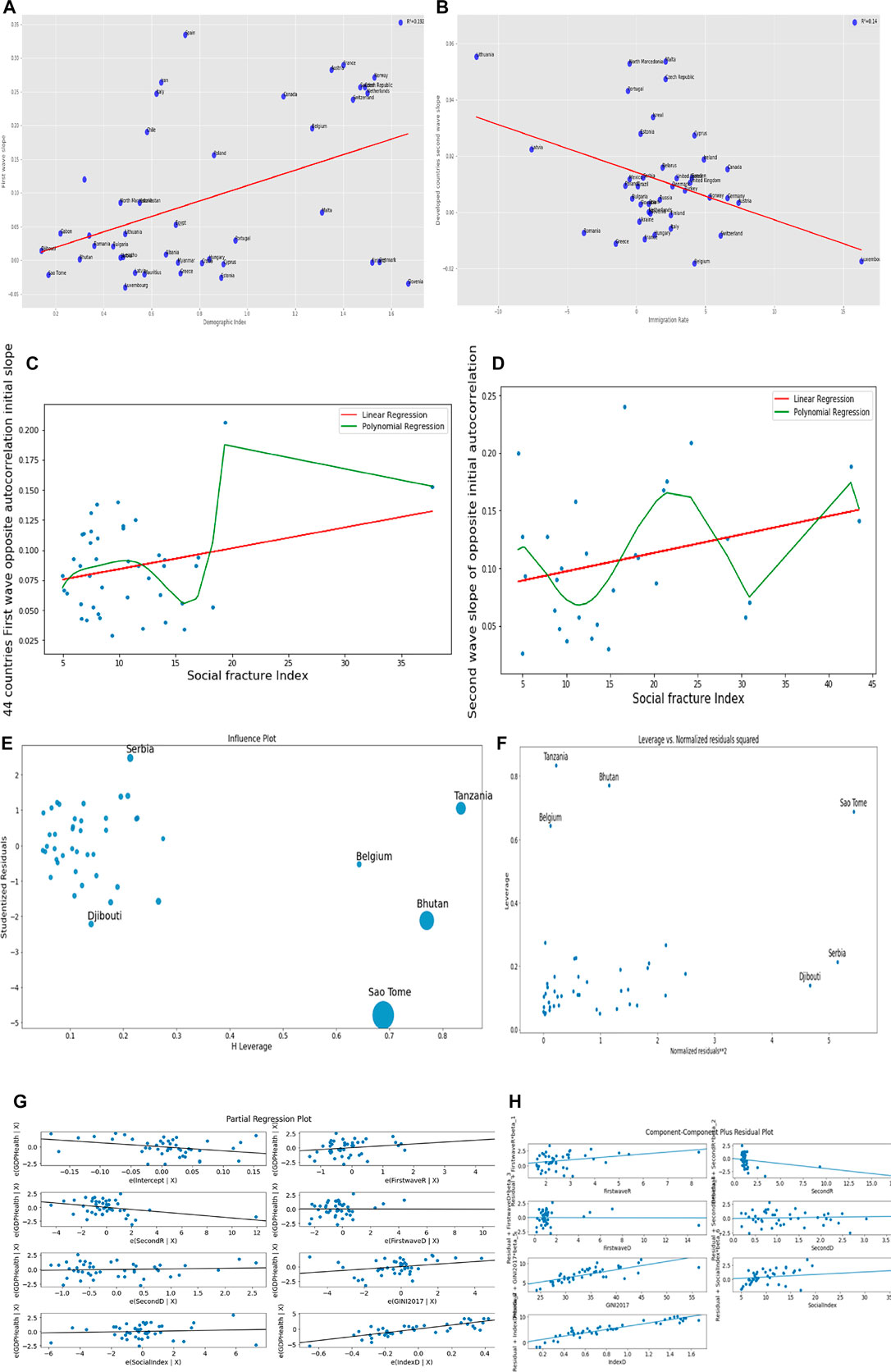
FIGURE 6. Linear regression plots for (A) the first wave slope vs. the demo-economic index for the developed and developing countries, (B) second wave slope vs. immigration rate for developed countries, (C) the opposite of the initial auto-correlation slope for first wave vs. social fracture index, (D) opposite of initial autocorrelation slope for second wave vs. social fracture index. (E) Influence plot. (F) Leverage vs. normalized residuals squared plot. (G) Partial regression plot. (H) Component–Component plus residual plot.

Figures 6E–H correspond to the ordinary multivariate least square method with R² = 0.76. Figure 6E shows some developing countries as outliers, while Belgium is the only developed country, which does not fit the data.

5.1.2 Prediction of Percentage GDP Devoted to Health Expenditure

In this section, we used a cross-validation method to choose the best parameter $\alpha$ for the modeling as shown in Figure 7C. For ridge regression, $\alpha =0.012$ with a mean square error = 2.32 and $\alpha =0.029$ for the lasso regression with a mean square error = 2.21. For Figure 7E, training score = 0.983 and test score = 0.607; for Figure 7F, training score = 0.170 and test score = 0.021; for Figure 7G, training score = 0.854 and test score = 0.115; and for Figure 7H, training score = 0.980 and test score = −2.386.

FIGURE 7

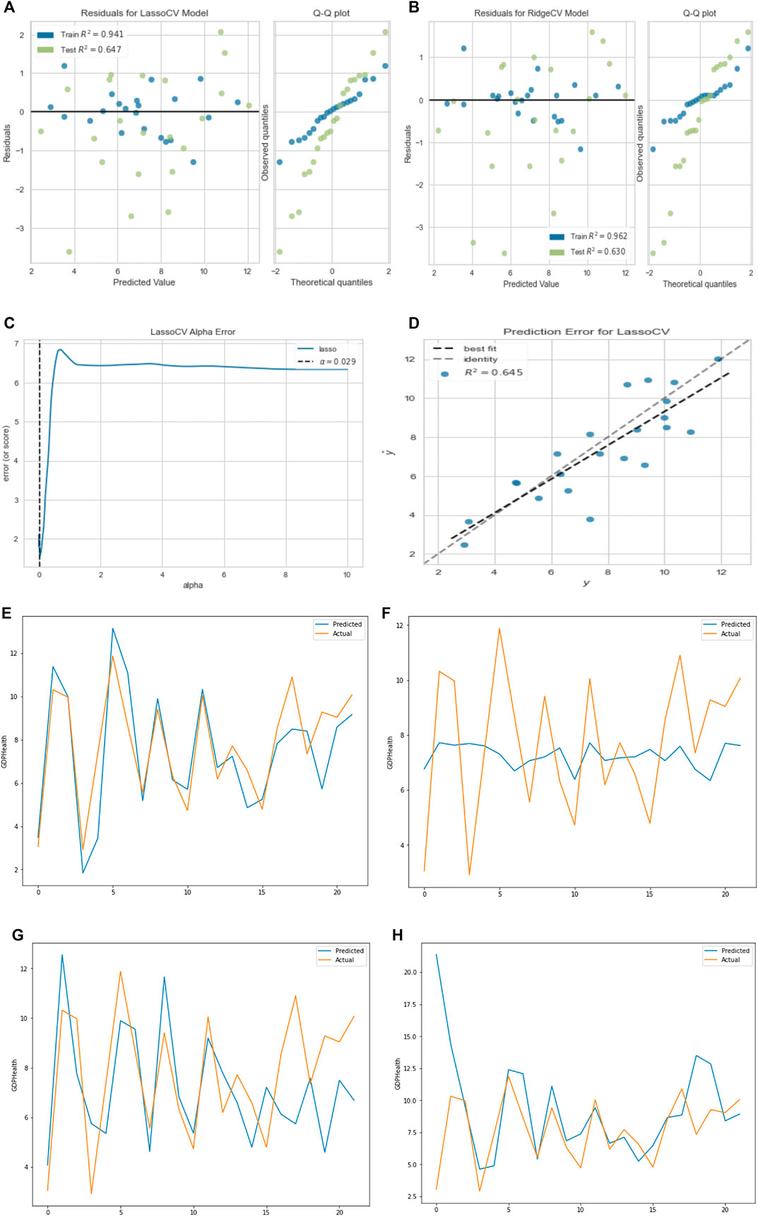
FIGURE 7. (A) Residual plot for lasso regression. (B) Residual plot for ridge regression. (C) Lasso regression cross-validation error. (D) Prediction error for lasso regression curve (R = 0.8). (E) Linear regression prediction plot. (E) Linear regression prediction plot. (F) Lasso regression prediction plot. (G) Ridge regression prediction plot. (H) MLP regression prediction plot.

It is evident from the results that linear regression best predicts GDP percentage devoted to health expenditure with the highest test score, and all predicted values are very close.

5.1.3 Principal Component Analysis and Clustering Results

In Figures 8E,F, the first cluster has 15 countries, the second cluster has 27 countries, while the last cluster has 2 countries, which are Tanzania and Mauritius. We only show the first two cluster dendrograms. With PC1, Gini index GI has the highest positive correlation of 0.52 with PC1 and demo-economic index DI has the second highest negative correlation of −0.53, while with PC2, first wave maximum R₀ has the highest positive correlation of 0.70 (Figure 8C).

FIGURE 8

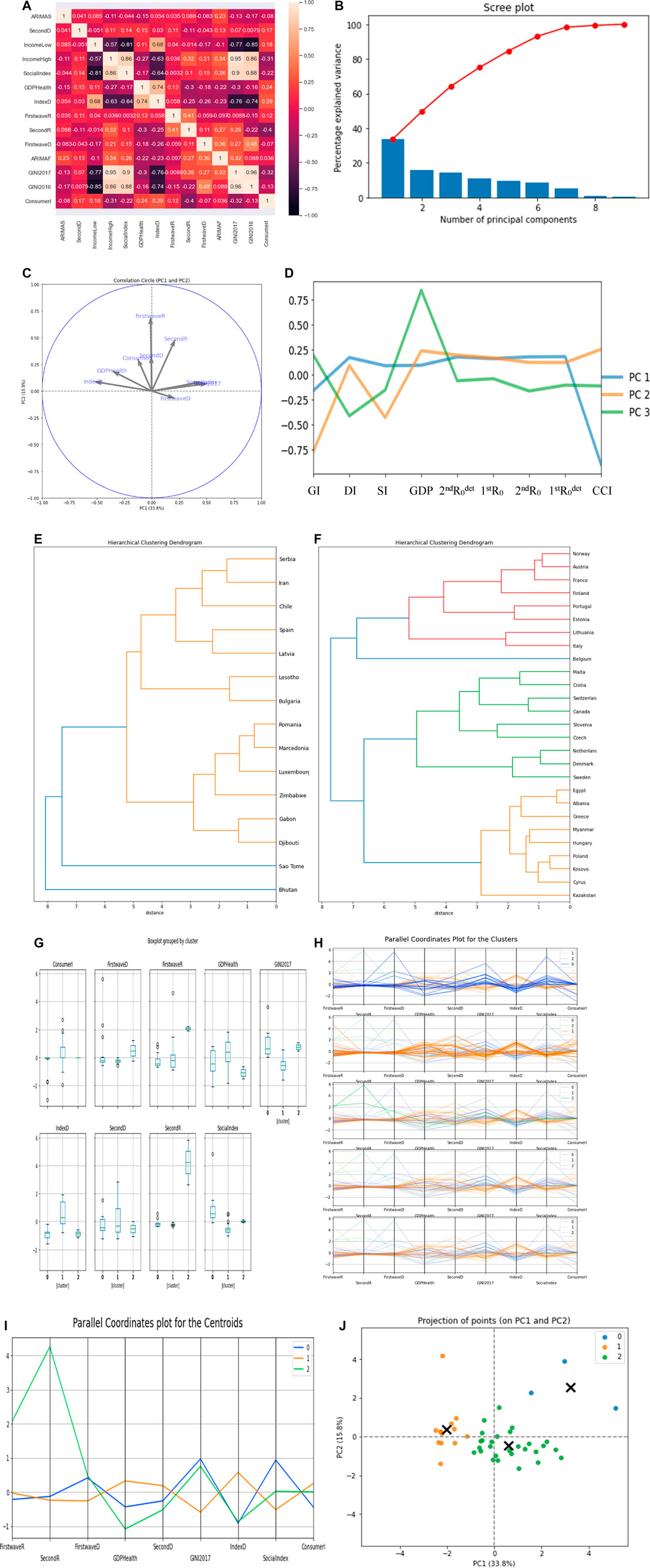
FIGURE 8. (A) Heatmap of the parameter’s correlations. (B) Scree plot. (C,D) PCs visualization.

The first cluster contains a majority of developing countries, and the second cluster contains a majority of developed countries, the main variable causing the separation into two classes being the Gini index in PC1.

5.2 African Countries

5.2.1 Multivariate Analysis for Socio-Economic Variables and Epidemiologic Variables

Figures 9A–D correspond to the ordinary multivariate least square method with R² = 0.60. Figure 9A shows Botswana and Tanzania as outliers not fitting the data.

FIGURE 9

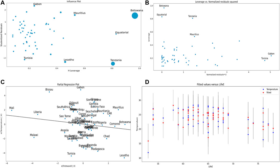
FIGURE 9. (A) Influence plot. (B) Leverage vs. normalized residuals squared plot. (C) Partial regression plot of the temperature vs. maximal R₀ of the first wave. (D) Fit plot. The first wave maximal R₀ is negatively correlated with the mean temperature of the country ([19,20]).

5.2.2 Prediction of Temperature

In this section, we used the cross-validation method to choose the best parameter $\alpha$ for the modeling as shown in Figure 10C. For ridge regression, $\alpha =1.005$ with a mean square error of 19.13, and for lasso regression, $\alpha =6.018$ with a mean square error = 16.93. For Figure 10E, training score = 0.647 and test score = −2.228; for Figure 10F, training score = 0.316 and test score = 0.154; for Figure 10G, training score = 0.573 and test score = −1.136; and for Figure 10H, training score = −6.728 and test score = −4.714. It is evident from these results that the lasso regression best predicts temperature with the highest test score, and predicted values of temperature for lasso and ridge regression are close.

FIGURE 10

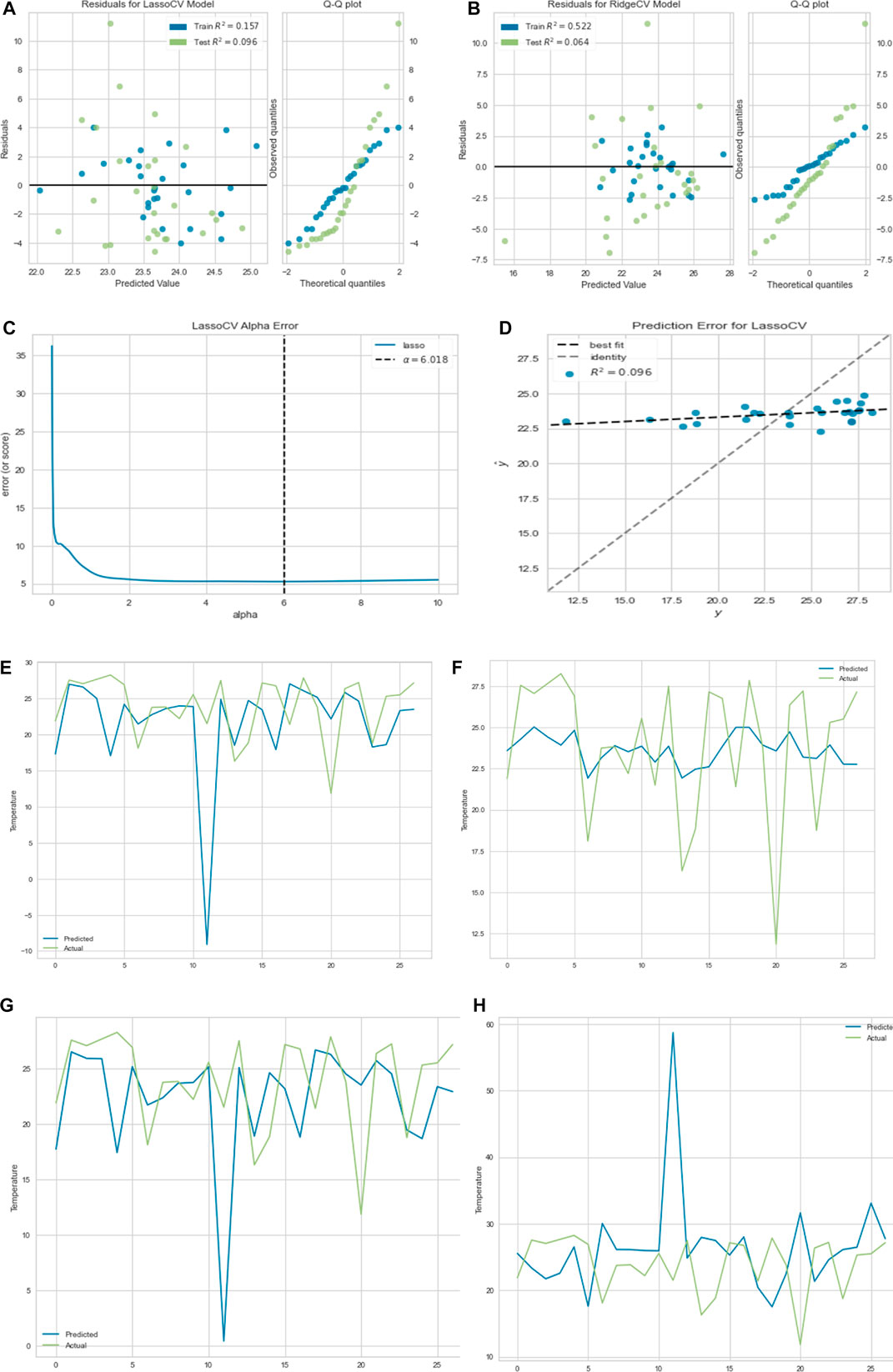
FIGURE 10. (A) Residual plot for lasso regression. (B) Residual plot for ridge regression. (C) Lasso regression cross-validation error. (D) Prediction error for lasso regression.

All the regression methods give about the same result with the maximum accuracy for the ridge regression.

5.2.3 Principal Component Analysis and Clustering Results

In Figures 11E,F, the first cluster has 40 countries, the second cluster has 13 countries, while the last cluster has only 1 country, which is Botswana. We only show the two cluster dendrograms with many countries. In Figure 11C, average life expectancy has the highest positive correlation of 0.46 in PC 1 while first wave deterministic ${\mathbf{R}}_{\mathbf{o}}$ (first wave D) has the highest positive correlation in PC 2, equal to 0.47.

FIGURE 11

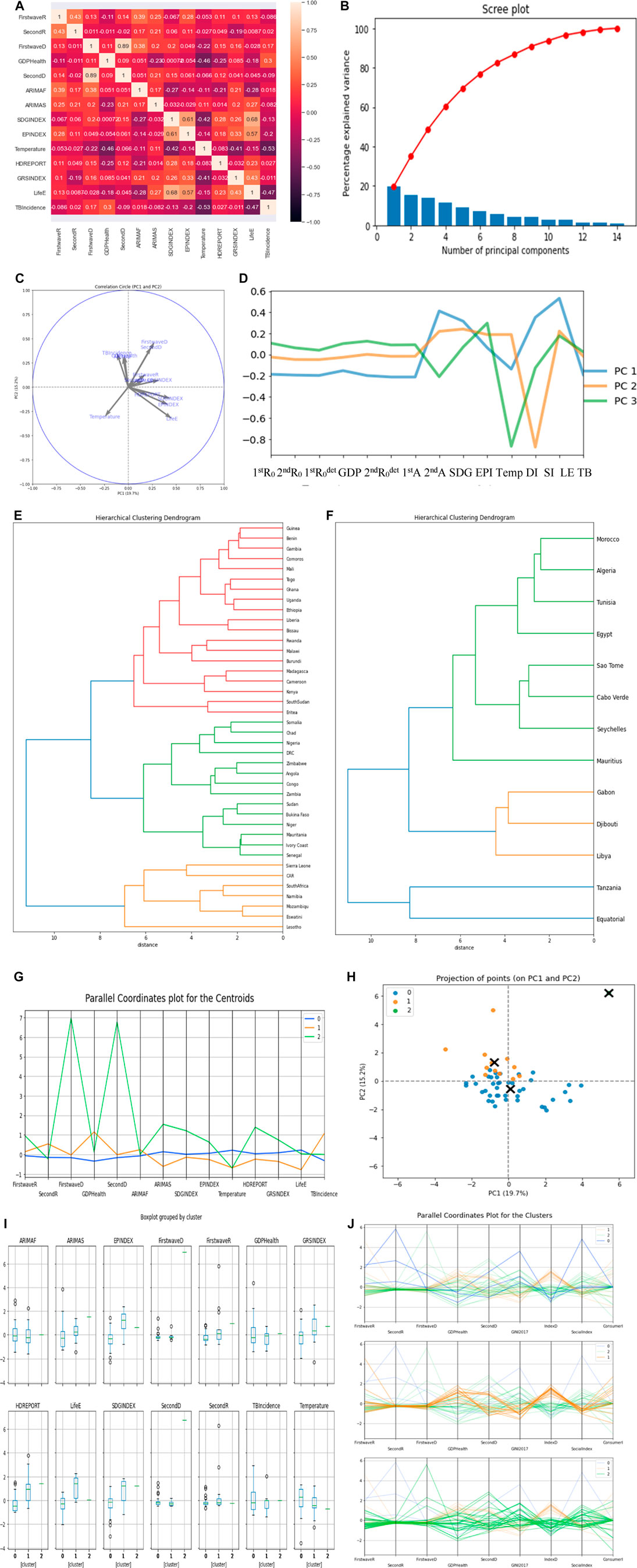
FIGURE 11. (A) Heatmap of the parameter’s correlations. (B) Scree plot. (C,D) PCs visualization.

The two socio-economic variables explaining the most clustering are the average life expectancy (LE) and the stringency index (SI).

5.3 OECD Countries

5.3.1 Multivariate Analysis for Socio-Economic Variables and Epidemiologic Variables

Figure 12 corresponds to the ordinary multivariate least square method with R² = 0.90. Figure 12A shows Iceland, United States, Austria, and Belgium as outliers not fitting the data.

FIGURE 12

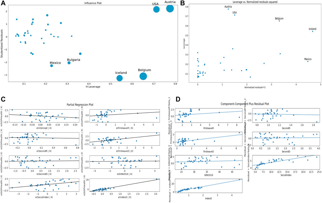
FIGURE 12. (A) Influence plot. (B) Leverage vs. Normalized residuals squared plot. (C) Partial regression plot. (D) Component–Component plus residual plot.

We see on the partial regression plots of the Figure 12C that the best correlation observed between parameters is between CHE/GDP and the demo-economic index DI as observed before in [21].

5.3.2 Prediction of Percentage GDP Health Expenditure

In this section, we used the cross-validation method to choose the best parameter $\alpha$ for the modeling as shown in Figure 13D. For ridge regression, $\alpha =0.005$ with a mean square error of 1.905, and for Lasso regression, $\alpha =0.027$ with a mean square error = 1.657. For Figure 13E, training score = 0.993 and test score = 0.535; for Figure 13F, training score = 0.898 and test score = 0.629; for Figure 13G, training score = 0.983 and test score = 0.259; and for Figure 13H, training score = −0.072 and test score = −0.196. It is evident from these results that the lasso regression best predicts percentage of GDP devoted to health expenditure with the highest test score and predicted values are very close.

FIGURE 13

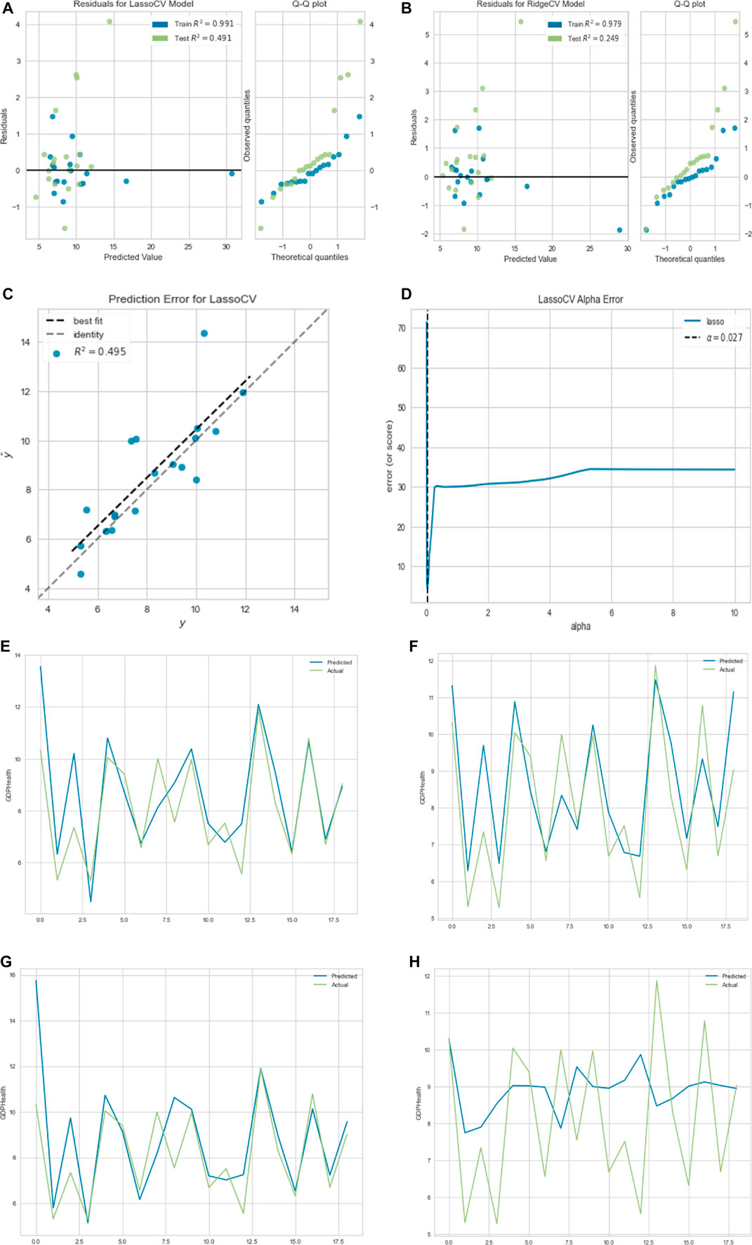
FIGURE 13. (A) Residual plot for lasso regression. (B) Residual plot ridge regression. (C) Prediction error for lasso regression. (D) Lasso regression cross-validation error.

All the regression methods give about the same result with the maximum accuracy for the ridge regression.

5.3.3 Principal Component Analysis and Clustering Results

In Figures 14E,F, the first cluster has 20 countries, and the second has 5 countries, which are United States and Bulgaria on the same hierarchy, Mexico and Costa Rica on the same hierarchy, and Chile standing alone. The third cluster has 12 countries. We only show the two highest cluster dendrograms. In Figure 14C, the Gini index and social fracture index have the highest positive correlation of 0.45 and 0.46, respectively, in PC 1 while the percentage of GDP devoted to health expenditure and demo-economic index have the highest positive correlation in PC 2, whose values equal to 0.65 and 0.41, respectively.

FIGURE 14

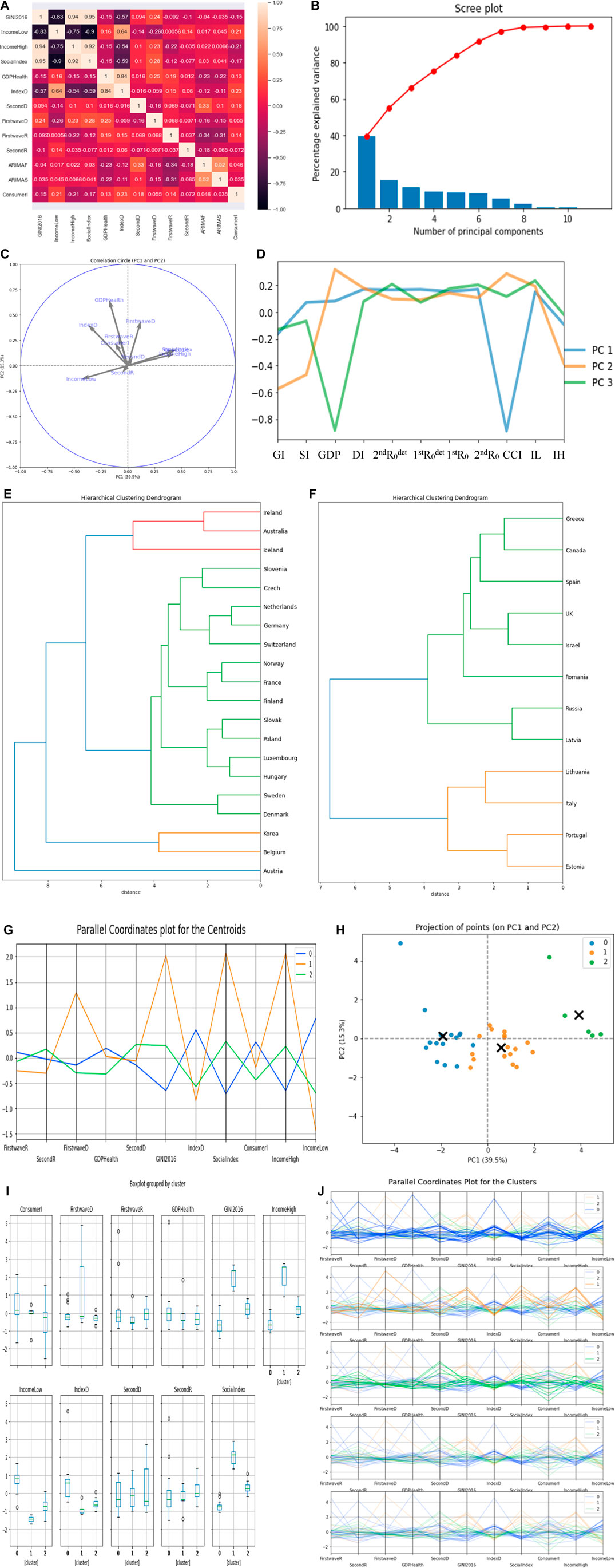
FIGURE 14. (A) Heatmap of the parameter’s correlations. (B) Scree plot. (C,D) PCs visualization.

The two main clusters correspond both to developed countries, but in the first, countries are more continental, and in the second, countries are more maritime, which could be explained by their difference in consumer confidence index (CCI), which is less important in maritime countries than in continental ones.

6 Discussion

We have been able to develop new approaches to the socio-economic determinants for the modeling of the COVID-19 pandemic during the exponential phase. Some of these determinants have shown high correlation with epidemiologic parameters as it can be seen in the heatmap diagrams in Figures 2G, 8A, 11A, 14A, explaining the role of each variable thanks to these correlations.

For developed and developing countries, the lasso regression reduced the correlation between the social fracture index and the 10% highest income, while for OECD countries, the correlation between the Gini index and social fracture index was reduced to zero. Some of our variables were not used in the optimization method-OLS due to multicollinearity observed on results summary. For the two sets of countries, consumer confidence index, opposite of the initial autocorrelation slope averaged on 6 days for the first and second wave, 10% lowest income, and 10% highest income were not used in the modeling. The R² for OLS results for developed, developing, and OECD countries are 0.76 and 0.90, respectively, which shows a high significance rate (Figures 8E,F, 12).

The principal component analysis shows high correlation for the numbers of new cases we used in this research. The social fracture index has high correlation in PC1 for both cases, while in PC2, percentage of GDP devoted to health expenditure was dominant for OECD countries, and maximum ${\mathbf{R}}_{\mathbf{o}}$ for the first wave was dominant for both developed and developing countries (see Figures 8C, 14C). We can deduce from all these observations that the socio-economic determinants are a key to the modeling of infectious diseases like COVID-19 as these parameters give high signals on the trend during the spread of the pandemic for various countries ([22–30]).

7 Conclusion

The systematic study of the correlations between socio-economic variables (Gini and Theil indices, percentage of GDP devoted to heath expenditure, etc.) and epidemiological variables (reproduction rate, opposite of the slope of autocorrelation to origin, etc.) shows a disparity between developed and developing countries, as well as between epidemic waves. Developed countries with high indices of social divide, but high health expenditure, did not, for the first wave, react better to the COVID-19 epidemic than developing countries. On the other hand, the rapid implementation of isolation and vaccination measures enabled them to anticipate and reduce the effects of the second wave. In a subsequent work, we will study the evolution of this disparity between developed and developing countries during subsequent waves of SARS CoV-2.

Data Availability Statement

The original contributions presented in the study are included in the article/Supplementary Material. Further inquiries can be directed to the corresponding author.

Author Contributions

Conceptualization, JD, KO, and MR. Methodology, JD, KO, and MR. Software, KO. Validation, JD; KO, and MR. Formal analysis, KO. Investigation, JD and MR. Resources, JD. Data curation, KO. Writing—original draft preparation, KO. Writing—review and editing, JD and KO. Visualization, KO. Supervision, JD and MR. Project administration, JD and MR. All authors have read and agreed to the final version of the manuscript.

Conflict of Interest

The authors declare that the research was conducted in the absence of any commercial or financial relationships that could be construed as a potential conflict of interest.

Publisher’s Note

All claims expressed in this article are solely those of the authors and do not necessarily represent those of their affiliated organizations, or those of the publisher, the editors, and the reviewers. Any product that may be evaluated in this article, or claim that may be made by its manufacturer, is not guaranteed or endorsed by the publisher.

Acknowledgments

The authors wish to acknowledge the Petroleum Technology Development Fund (PTDF) Nigeria doctoral fellowship in collaboration with Campus France Africa Unit.

Supplementary Material

The Supplementary Material for this article can be found online at: https://www.frontiersin.org/articles/10.3389/fams.2021.786983/full#supplementary-material

References

1. Demongeot, J, Oshinubi, K, Rachdi, M, and Seligmann, H. Geoclimatic, Demographic and Socio-Economic Determinants of the Covid-19 Prevalence. EGU Gen Assembly (2021) EGU21-7976. doi:10.5194/egusphere-egu21-7976

CrossRef Full Text | Google Scholar

2. Barlow, J, and Vodenska, I. Socio-Economic Impact of the Covid-19 Pandemic in the U.S. Entropy (2021) 23:673. doi:10.3390/e23060673

PubMed Abstract | CrossRef Full Text | Google Scholar

3. Ahmed, HM, Elbarkouky, RA, Omar, OAM, and Ragusa, MA. Models for COVID-19 Daily Confirmed Cases in Different Countries. Mathematics (2021) 9:659. doi:10.3390/math9060659

CrossRef Full Text | Google Scholar

4. Kong, JD, Tekwa, EW, and Gignoux-Wolfsohn, SA. Social, Economic, and Environmental Factors Influencing the Basic Reproduction Number of COVID-19 across Countries. PLoS ONE (2021) 16:e0252373. doi:10.1371/journal.pone.0252373

PubMed Abstract | CrossRef Full Text | Google Scholar

5. Qiu, Y, Chen, X, and Shi, W. Impacts of Social and Economic Factors on the Transmission of Coronavirus Disease 2019 (COVID-19) in China. J Popul Econ (2020) 33:1127–72. doi:10.1007/s00148-020-00778-2

PubMed Abstract | CrossRef Full Text | Google Scholar

6. Oshinubi, K, Rachdi, M, and Demongeot, J. Analysis of Reproduction Number R0 of COVID-19 Using Current Health Expenditure as Gross Domestic Product Percentage (CHE/GDP) across Countries. Healthcare (2021) 9:1247. doi:10.3390/healthcare9101247

PubMed Abstract | CrossRef Full Text | Google Scholar

7.World bank. World Bank (2021). Available at: https://data.worldbank.org/(accessed on February 12, 2021).

Google Scholar

8.OECD. Organisation for Economic Co-operation and Development (2021). Available at: https://data.oecd.org/(accessed on February 12, 2021).

Google Scholar

9.SDSN. 2019 Africa SDG Index and Dashboards Report (2021). Available at: https://www.sdgindex.org/reports/2019-africa-sdg-index-and-dashboards-report/(accessed on February 22, 2021).

Google Scholar

10.UNDP. Adjusted Net Savings (% of GNI) Dimension: Socio-Economic Sustainability (2021). Available at: http://hdr.undp.org/en/indicators/164406 (accessed on February 22, 2021).

Google Scholar

11.Our World in Data. Covid-Stringency (2021). Available at: https://ourworldindata.org/grapher/covid-stringency-index?tab=table (accessed on February 22, 2021).

Google Scholar

12.Wikipedia. List of Countries by Average Yearly Temperature (2021). Available at: https://en.wikipedia.org/wiki/List_of_countries_by_average_yearly_temperature (accessed on February 22, 2021).

Google Scholar

13.Statista. Life Expectancy at Birth in Africa as of 2019, by Country (2021). Available at: https://www.statista.com/statistics/1218173/life-expectancy-in-african-countries/(accessed on February 22, 2021).

Google Scholar

14.EPI. Environmental Performance Index (2021). Available at: https://epi.yale.edu/(accessed on February 22, 2021).

Google Scholar

15.Wikipedia. List of Countries by Net Migration Rate (2021). Available at: https://en.wikipedia.org/wiki/List_of_countries_by_net_migration_rate (accessed on February 22, 2021).

Google Scholar

16.Wikipedia. Coefficient de Gini (2021). Available at: https://fr.wikipedia.org/wiki/Coefficient_de_Gini (accessed on August 22, 2021).

Google Scholar

17.Wikipedia. Indice de Theil (2021). Available at: https://fr.wikipedia.org/wiki/Indice_de_Theil (accessed on August 22, 2021).

Google Scholar

18.Institute of Global Health. COVID-19 Daily Epidemic Forecasting (2021). Available at: https://renkulab.shinyapps.io/COVID-19-Epidemic-Forecasting/_w_f1413dad/?tab=jhu_pred&country= (accessed on September 22, 2021).

Google Scholar

19. Demongeot, J, Flet-Berliac, Y, and Seligmann, H. Temperature Decreases Spread Parameters of the New Covid-19 Case Dynamics. Biology (2020) 9:94. doi:10.3390/biology9050094

PubMed Abstract | CrossRef Full Text | Google Scholar

20. Seligmann, H, Iggui, S, Rachdi, M, Vuillerme, N, and Demongeot, J. Inverted Covariate Effects for Mutated 2^nd vs 1^st Wave Covid-19: High Temperature Spread Biased for Young. Biology (Basel) (2020) 9:226. doi:10.3390/biology9080226

PubMed Abstract | CrossRef Full Text | Google Scholar

21. Demongeot, J, Noury, N, and Vuillerme, N. Data Fusion for Analysis of Persistence in Pervasive Actimetry of Elderly People at home. In: IEEE ARES-CISIS' 08. Piscataway: IEEE Proceedings (2008). p. 589–94.

Google Scholar

22. Demongeot, J, and Seligmann, H. SARS-CoV-2 and miRNA-like Inhibition Power. Med Hypotheses (2020) 144:110245. doi:10.1016/j.mehy.2020.110245

PubMed Abstract | CrossRef Full Text | Google Scholar

23. Demongeot, J, Griette, Q, and Magal, P. Computations of the Transmission Rates in SI Epidemic Model Applied to COVID-19 Data in mainland China. R Soc Open Sci (2020) 7:201878. doi:10.1098/rsos.201878

PubMed Abstract | CrossRef Full Text | Google Scholar

24. Soubeyrand, S, Demongeot, J, and Roques, L. Towards Unified and Real-Time Analyses of Outbreaks at Country-Level during Pandemics. One Health (2020) 11:100187. doi:10.1016/j.onehlt.2020.100187

PubMed Abstract | CrossRef Full Text | Google Scholar

25. Gaudart, J, Landier, J, Huiart, L, Legendre, E, Lehot, L, Bendiane, MK, et al. Factors Associated with the Spatial Heterogeneity of the First Wave of COVID-19 in France: a Nationwide Geo-Epidemiological Study. The Lancet Public Health (2021) 6:e222–e231. doi:10.1016/s2468-2667(21)00006-2

PubMed Abstract | CrossRef Full Text | Google Scholar

26. Oshinubi, K, Al-Awadhi, F, Rachdi, M, and Demongeot, J. Data Analysis and Forecasting of COVID-19 Pandemic in Kuwait. Kuwait J. Sci. (2021), Special Issue 1–28. doi:10.48129/kjs.splcov.14501

CrossRef Full Text | Google Scholar

27. Griette, Q, Demongeot, J, and Magal, P. A Robust Phenomenological Approach to Investigate COVID-19 Data for France. Math Appl Sci Eng (2021) 2:149–60. doi:10.5206/mase/14031

CrossRef Full Text | Google Scholar

28. Oshinubi, K, Rachdi, M, and Demongeot, J. Functional Data Analysis: Transition from Daily Observation of COVID-19 Prevalence in France to Functional Curves. MedRxiv (2021). doi:10.1101/2021.09.25.21264106

CrossRef Full Text | Google Scholar

29. Demongeot, J, Oshinubi, K, Rachdi, M, Hobbad, L, Alahiane, M, Iggui, S, et al. The Application of ARIMA Model to Analyse Incidence Pattern in Several Countries. J Math Comput Sci (2021) 26:41–57. doi:10.28919/jmcs/6541

CrossRef Full Text | Google Scholar

30. Demongeot, J, Oshinubi, K, Rachdi, M, Seligmann, H, Thuderoz, F, and Waku, J. Estimation of Daily Reproduction Numbers during the COVID-19 Outbreak. Computation (2021) 9:109. doi:10.3390/computation9100109

CrossRef Full Text | Google Scholar