Flexible time-to-event models for double-interval-censored infectious disease data with clearance of the infection as a competing risk

1. Introduction

In infectious disease research one is often interested in the association between some biological variables and a time-to-event outcome, defined as the time from a starting point or origin event until the event of interest. Some examples of such outcomes are the time from birth to childhood pneumonia [1], the time from hospitalization of COVID-19 patients to mortality [2], or the time from incident malaria infection to initiation of gametocyte production [3, 4]. The analysis of this type of data may vary in complexity due to, for instance, missing time-to-event data by different types of censoring or the presence of competing risks. In particular, when the origin event is an initial infection and one is interested in the induction time until another event of interest, clearance or resolution of the initial infection is a competing risk. The time from HIV infection to the onset AIDS is a well known example [5]. While HIV infection may not clear completely, due to treatment it can reach undetectable levels thus mitigating the risk of AIDS onset. If individuals are only routinely followed-up the data are often double-interval-censored which gives an additional layer of complexity in the analysis. In this paper we focus on methodology for analyzing this kind of data. As an illustrative example, described in Section 4, we study the time from incident malaria infection to initiation of the transmissible stages (gametocytes) that, for Plasmodium falciparum, show delayed appearance. Individuals visit a clinic at regular time points at which they are tested for malaria infection and initiation of gametocyte production in case of an infection. The aim is to estimate the hazards over the latent time from infection to gametocyte production. In this example this time-span is double-interval-censored and often missing due to clearance of the infection (competing risk).

1.1. What are right- and double-interval-censoring?

Right-censoring, the most commonly occurring type of censoring, happens when the event of interest is not observed, but is known to happen after a certain time-point, for instance after the end of the study period. In most longitudinal infectious disease studies individual data are routinely collected at regular time points, like visits to a clinic. At these visits it is observed whether an individual has already experienced the event or not. Then, the exact time of an event is not observed, but rather known to be occurred between two visits. This type of censoring is known as interval-censoring. If the start time is interval-censored as well, for instance if the origin event is an initial infection, the data are double-interval-censored. A well-known example of double-interval-censored data in literature is the study of AIDS induction time, i.e., the time from HIV infection to onset of AIDS. The time of HIV infection and the time of onset of AIDS are both interval-censored [6–8]. Also in the illustrating malaria data we have to deal with double-interval-censoring: the time of malaria infection and the time of initiation of gametocyte production are both interval-censored.

1.2. What are competing risks?

In survival analysis we often have to deal with a competing event, i.e., an event that prevents the event of interest from being observed [9]. This happens for many infectious diseases where the origin event (infection) can be cleared before the event of interest is observed. For instance, in the malaria data in which we are interested in studying the time from infection to gametocyte production, the infection might be cleared before gametocyte initiation. Therefore, clearance of the infection can be treated as a competing event. When competing events are present in the data, they should be modeled as such using competing risks models [9, 10]. For infections that cannot resolve, like HIV, death could be seen as a competing event.

1.3. Aim of the paper

To the best of our knowledge there is no available literature on regression models for modeling competing events with double-interval-censored data, and no available software. Adamic [11] looked at non-parametric modeling of double-censored data with competing risks but did not consider interval-censored data. Sankaran and Sreedevi [12] looked at a model for double-censored data (also not considering interval-censoring) with competing risks using an extension of the Gray [13] approach. In this paper we aim to develop and compare models for double-interval-censored competing risks data of infectious diseases. We restrict ourselves to situation in which one is interested in the time from infection to an event of interest with clearance of the infection as a competing risk. We illustrate the methodology through a simulation study and through a real-world example in malaria transmission epidemiology. Through the simulation study we also show how well these models compare to standard competing risks models when the exact times are observed (or right-censored) instead of interval-censored. Through the malaria example, we show how these models can be applied to infectious diseases data where the start time, which is not known exactly, is defined by an infection that can be cleared. We share available code for reproducing such analyses.

1.4. Overview of the paper

In Section 2, we describe the methodology for analyzing double-interval-censored data with competing events. We propose different statistical models for the analysis. Thereafter, in Section 3, we examine and compare the performance of these models under various scenarios with a simulation study. In Section 4, we look at the illustrative example using malaria transmission data. We end the paper with a discussion and conclusion in Section 5.

2. Methods

2.1. Short introduction to survival analysis

Let the survival time T be a non-negative continuous random variable representing the time from an origin event until the time of an event of interest. The survival function S(t) = P(T>t) is defined as the probability the event happens after time t and equals the compliment of the cumulative incidence at time t. It is either estimated non-parametrically by the Kaplan-Meier estimator or through its relationship with the hazard function λ, i.e., S(t) = exp[−Λ(t)] where $\Lambda (t)=\underset{0}{\overset{t}{\int }}\lambda (s)ds$ is the cumulative hazard function. The hazard function is the instantaneous rate at which an individual experiences an event of interest over time conditional that he/she has remained event-free until that time, i.e.,

$\lambda (t)={\displaystyle \underset{dt\to 0}{lim}}\frac{P(t\le T<t+dt|T\ge t)}{dt}.$

In regression modeling, where we aim to study the relationship between a covariate vector x and the survival time T, the emphasis is on the hazard function. The most commonly used regression model for time-to-event data is the Cox proportional hazards (CPH) model [14]. In this semi-parametric model the hazard function is defined as $\lambda (t)={\lambda }_0(t)exp({\beta }^{{}^{\prime }}\text{x})$, where β is the vector of unknown regression parameters and λ₀ the unknown baseline hazard function. The model assumes that covariate effects β are constant over time [i.e., proportional hazards (PH)]. Flexible models that address violations in the proportional hazards assumption with applications to infectious diseases have been discussed in greater detail [15, 16]. Many other extensions of the CPH model have been proposed to accommodate complexities in the data generating mechanisms and/or the data collection limitations such as left-truncation, left-censoring, interval-censoring, competing risks, recurrent events, etc. [17–21], but in none of them the combination of double-interval-censoring and competing risks, which regularly is the case in infectious disease data, is studied.

2.2. Specification of the baseline hazard function λ₀(t)

The baseline hazard function can be specified through a parametric distribution for the survival time T. The exponential and the Weibull distributions are common (and easily implemented) specifications. An exponential distribution assumes that the baseline hazard rate is constant over time, while a Weibull distribution implies a monotonically increasing/decreasing baseline hazard [22]. The parametric forms of these distributions, while useful, may be too simple for the true baseline hazards which may lead to biases in the estimated covariate effects. A spline based model for the baseline hazards gives much more flexibility, so much so that these models are often considered non-parametric [23]. Flexible models using penalized splines are gaining momentum in advanced survival analysis models [15, 16, 24].

For the exponential model the baseline hazards is specified as a constant, i.e.,

${\lambda }_0(t)=\lambda$

where λ>0. Its cumulative baseline hazard equals Λ₀(t) = λt. The Weibull specification is

${\lambda }_0(t)=\rho {\lambda }^{\rho }{t}^{\rho -1}$

where λ, ρ>0. Note, when ρ = 1 it reduces to an exponential baseline hazard. The cumulative baseline hazard is ${\Lambda }_0(t)={(\lambda t)}^{\rho }$. The B-spline baseline hazard function is given by a linear combination of m B-spline basis functions and a set of corresponding coefficients, i.e.,

${\lambda }_0(t)={\displaystyle \sum _{j=1}^m}{\theta }_j{b}_j(t)$

where θ_j>0. The cumulative baseline hazard can be specified using higher order B-splines basis functions as an approximation to the integrated B-splines basis functions [25] such that

${\text{Λ}}_0(t)={\displaystyle \sum _{j=1}^m}{\theta }_j{B}_j(t)$

where B_j are integrated B-splines basis functions. According to Wood [26] and other authors [15, 16], m = 10 is usually sufficient for good estimation.

2.3. A competing risks model

Competing events are events that prevent the event of interest from being observed. They are easily modeled in a framework that redefines the survival function as the probability of not experiencing either the event of interest or the competing event before time t, and defining cumulative incidences for each event as the measure of interest (the probability of experiencing each event over time). Ignoring a competing event (i.e., by considering the time that competing event occurs as right-censored) results in inflated cumulative incidences for the event of interest [9, 10] as well as a missing piece of information in the transmission epidemiology. We use the multi-state approach for modeling competing risks [27]. Here we model the effects of covariates on the cause-specific hazard rates.

As shown in Figure 1, we define two hazard rates: one for the time from infection to the event of interest, ${\lambda }_1(t|{\text{x}}_1)={\lambda }_{01}(t)exp({\text{β}}_1^{\prime }{\text{x}}_1)$, and one for the time from infection to its clearance (the competing risk), ${\lambda }_2(t|{\text{x}}_2)={\lambda }_{02}(t)exp({\text{β}}_2^{\prime }{\text{x}}_2)$. Here λ₀₁ and λ₀₂ are the baseline hazard functions for both events. For each event k, k = 1, 2, x_k is a vector of covariates and β_k is a vector of regression coefficients to be estimated. The cumulative hazard rates for event k is

${\Lambda }_k(t|x_k)={\Lambda }_{0k}(t)\exp ({\beta }_k^{\prime }{x}_k)\text{ with }{\Lambda }_{0k}(t)={\displaystyle {\int }_0^t{\lambda }_{0k}}(u)du.$

FIGURE 1

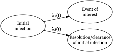
Figure 1. Competing risks model for two events, a main event of interest from an initial infection and clearance/resolution of the initial infection without the main event of interest.

The marginal survival probability (probability of not experiencing either event before time t) is given by

$S(t|{\text{x}}_1,{\text{x}}_2)=exp(-{\text{Λ}}_1(t|{\text{x}}_1)-{\text{Λ}}_2(t|{\text{x}}_2))$

and the cumulative incidence probabilities up to time t for event k is given by

$P_k(t|x_1,x_2)={\displaystyle {\int }_0^{t}S}(u-|x_1,x_2){\lambda }_k(u|x_k)du.$

2.4. Interval-censoring and double-interval-censoring

As mentioned before, a survival time is interval-censored if the exact time is not observed, but known to lie within an interval. In many applications researchers ignore interval-censoring in the data by using the midpoint or the right-end point of the interval as the exact observed event time. This usually leads to biased estimates of the regression parameters and of the standard error [28–30]. In the case of double-interval-censoring these issues may be more pronounced.

In the likelihood the interval-censoring is dealt with by integrating over the interval in which the event occurred. If the time of the origin event is observed and the time from this origin event to the event of interest is known to fall in an interval (L, R) its leverage to the likelihood function is $\underset{L}{\overset{R}{\int }}f(s|\text{x})ds=S(L|\text{x})-S(R|\text{x})$ where f(t|x) is the conditional density of T. Then the full likelihood for n individuals is given by the product

$\begin{array}{l}L(\beta |x)={\displaystyle \prod _{i=1}^n{\displaystyle {\int }_{L_i}^{R_i}f}}(s|x_i)ds\\ ={\displaystyle \prod _{i=1}^{n}S}(L_i|x_i)-S(R_i|x_i).\end{array}$

where i indicates the individual.

Parameters are estimated by maximizing the log-likelihood function. This is straightforward when the baseline hazard function is specified. Flexible models for dealing with interval-censoring using splines for baseline hazards specification are becoming increasingly popular [24, 31, 32].

In this paper, we consider double-interval-censored data. To illustrate different scenarios of the time-to-event data, the longitudinal follow-up data in calendar time of three individuals is presented in the upper panel of Figure 2. Participant 1 has an interval-censored infection time (infection occurred between L₀ and R₀) and is right-censored for the event of interest at time L₁—we do not observe an event time for this participant but we know that it had not happened before the time of the last follow-up visit at L₁. Participant 2 has an interval-censored infection time (infection happened between L₀ and R₀) and time of the event of interest (happened between L₁ and R₁), and participant 3 has an interval-censored infection time and event of interest time and the observation intervals overlap completely (both events occurred between L₀ = L₁ and R₀ = R₁). In general, L₀ is the date of the last visit before infection, R₀ is the date of the visit when the infection was confirmed to have happened before, L₁ is either the date of the last visit prior to the event of interest (or clearance of the infection) or the date of last follow-up when no event or clearance was observed (right-censored), and R₁ is the date of the visit at which it is being confirmed that the event have occurred before. For right censored data R₁ is not observed. The data in the upper panel of Figure 2 are in calendar time. For the analysis of the data we transform these calendar data to follow-up data by defining a starting point at which the follow-up time starts. The starting point t₀: = 0 is defined as the last observed moment infection had not yet taken place (so L₀ in the upper panel). By this transformation new intervals for the events are defined as can be seen in the middle panel of Figure 2; (t₀, t₁) for the infection time and (t₂, t₃) for the event of interest. For the third scenario where the two intervals overlap, we specifically note that t₂ = t₀: = 0 and t₃ = t₁. For right censored data t₃ = ∞. In the middle panel of Figure 2, we denote the unobserved times for infection and the event of interest by W and U. By definition W∈(t₀, t₁), U∈(t₂, t₃) and the unobserved survival time is T = U−W. The admissible survival times (T) for the three participants given the intervals (t₀, t₁) and (t₂, t₃) are shown in the lower panel of Figure 2. In some studies, a simple transformation of double-interval-censored data into single interval-censored data have been used, i.e., the time from (L₀, R₀) to (L₁, R₁) is converted to (L₁−R₀, R₁−L₀). De Gruttola and Lagakos [7] argues that this is not appropriate and is only valid when the density function for the time to the origin event is uniform in chronological time. In our likelihood formulation described in Section 2.5, we assume that the infection time is uniformly distributed within the interval (L₀, R₀) and make no assumptions about the density function for the time to the origin event prior to L₀.

FIGURE 2

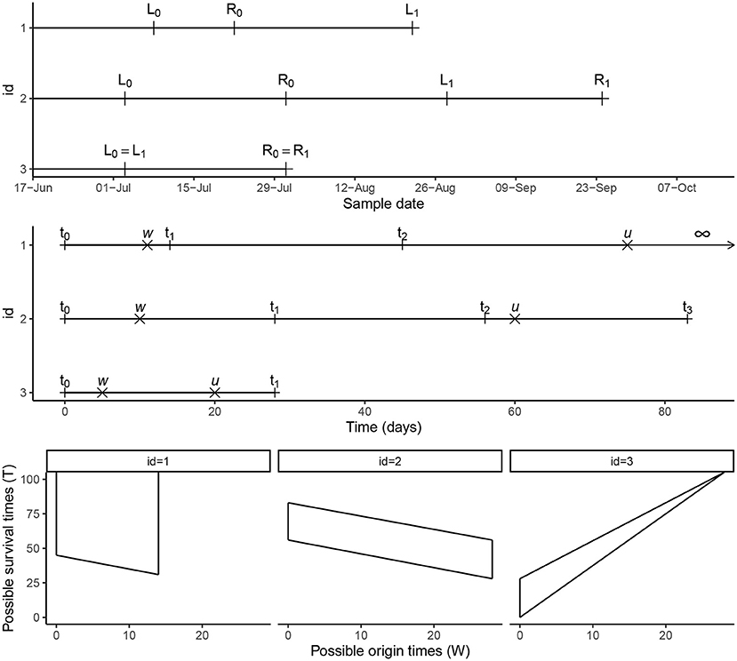
Figure 2. Timeline. Conversion of calendar time data into follow-up time intervals for three participants from the malaria cohort and the possible survival times (T) representing the time from the initial infection to the event of interest.

A few methods that take double-interval-censoring into account in their analysis have been proposed: these can be described as non-parametric approaches [7], proportional hazards approaches [33, 34], and multiple imputation approaches [35] among others. Kim et al. [33] proposed a discrete time proportional hazards model in an extension of the Turnbull [36] estimator. In their work, Sun et al. [34] estimated the effects of covariates in a proportional hazards framework using estimating equations. However, they focused on interval-censored start times with an exactly observed or right-censored event-times. In the presence of a few interval-censored event times, they assumed the time exactly equal to the right-boundary of the interval and performed some sensitivity analysis. Sun [6] gives an overview of some of these approaches and discuss issues related to them with a focus on left truncation and also proportional hazards violations. In this paper, we look at modeling the hazard rates in a regression modeling approach for continuous time-to-event data. The baseline hazards are specified by well-known parametric distributions or more flexible shapes using B-splines. Estimation involves maximizing the full-likelihood or penalized likelihood when using splines. This is the topic of the next subsection.

2.5. Likelihood function and estimation

For individual i we observe the data Ω_i = (t_0i = 0, t_1i, t_2i, t_3i, δ_1i, δ_2i, α_i, x₁, x₂), with t_0i, t_1i, t_2i, t_3i as defined in the previous subsection. The functions δ_1i and δ_2i indicate whether the event of interest or the competing event (clearance of the infection) has occurred: (δ_1i, δ_2i) = (1, 0) for the event of interest, (δ_1i, δ_2i) = (0, 1) for the competing event, (δ_1i, δ_2i) = (0, 0) none occurred (the data are right-censored) and (δ_1i, δ_2i) = (1, 1) is not possible by definition. For right-censored data t_3i: = ∞. We also define α_i = I[(t_0i, t_1i) = (t_2i, t_3i)] to indicate whether or not the event of interest was observed in the same interval as the infection. We assume that the observation intervals are sufficiently narrow to exclude the case in which infection and its clearance happen in the same interval, so that all infections are observed. Not making this assumption would complicate the methodology dramatically, as then latent infections could happen in any interval. In the malaria example the assumption is likely satisfied. The vectors x₁ and x₂ are observed covariates that might be associated with the time to the event of interest and to the competing event.

We assume that the times of the visits in calendar time (observation times of the individuals) are statistically independent of the actual unobserved event times U and W (and of the competing event). By this assumption, it is reasonable to assume that time to infection W within the interval (t_0i = 0, t_1i) (given t_1i) follows a uniform distribution at this interval with the density $f(w)=\frac{1}{t_{1i}}$.

In the following, we derive the likelihood function for the observed data of individual i (conditional all observation (visit times)). First, we do this for the four possible scenario's indicated by δ_1i, δ_2i, and α_i. The full likelihood for individual i can be found by combining these four terms.

Right censored, no overlap (δ_1i = 0, δ_2i = 0, α_i = 0)

$L_i=\left(\frac{1}{t_{1i}}\right){\displaystyle {\int }_0^{t_{1i}}\exp }(-{\text{Λ}}_1(t_{2i}-w)-{\text{Λ}}_2(t_{2i}-w))dw,$

Competing event, no overlap (δ_1i = 0, δ_2i = 1, α_i = 0)

$L_i=\left(\frac{1}{t_{1i}}\right){\displaystyle {\int }_0^{t_{1i}}{\displaystyle {\int }_{t_{2i}}^{t_{3i}}\exp }}(-{\text{Λ}}_1(u-w)-{\text{Λ}}_2(u-w)){\lambda }_2(u-w)dudw,$

Event of interest, no overlap (δ_1i = 1, δ_2i = 0, α_i = 0)

$L_i=\left(\frac{1}{t_{1i}}\right){\displaystyle {\int }_0^{t_{1i}}{\displaystyle {\int }_{t_{2i}}^{t_{3i}}\exp }}(-{\text{Λ}}_1(u-w)-{\text{Λ}}_2(u-w)){\lambda }_1(u-w)dudw,$

Event of interest, with overlap (δ_1i = 1, δ_2i = 0, α_i = 1)

$L_i=\left(\frac{1}{t_{1i}}\right){\displaystyle {\int }_0^{t_{1i}}{\displaystyle {\int }_w^{t_{1i}}\exp }}(-{\text{Λ}}_1(u-w)-{\text{Λ}}_2(u-w)){\lambda }_1(u-w)dudw.$

The resulting log-likelihood is thus

$\begin{array}{l}l(\varphi |{\Omega }_i)=(1-{\delta }_{1i})(1-{\delta }_{2i})(1-{\alpha }_i)\\ \log \left({\displaystyle {\int }_0^{t_{1i}}\exp }(-{\text{Λ}}_1(t_{2i}-w)-{\text{Λ}}_2(t_{2i}-w))dw\right)\\ +(1-{\delta }_{1i}){\delta }_{2i}(1-{\alpha }_i)\\ \log \left({\displaystyle {\int }_0^{t_{1i}}{\displaystyle {\int }_{t_{2i}}^{t_{3i}}\exp }}(-{\text{Λ}}_1(u-w)-{\text{Λ}}_2(u-w)){\lambda }_2(u-w)dudw\right)\\ +{\delta }_{1i}(1-{\delta }_{2i})(1-{\alpha }_i)\\ \log \left({\displaystyle {\int }_0^{t_{1i}}{\displaystyle {\int }_{t_{2i}}^{t_{3i}}\exp }}(-{\text{Λ}}_1(u-w)-{\text{Λ}}_2(u-w)){\lambda }_1(u-w)dudw\right)\\ +{\delta }_{1i}(1-{\delta }_{2i}){\alpha }_i\\ \log \left({\displaystyle {\int }_0^{t_{1i}}{\displaystyle {\int }_w^{t_{1i}}\exp }}(-{\text{Λ}}_1(u-w)-{\text{Λ}}_2(u-w)){\lambda }_1(u-w)dudw\right)\\ -\log (t_{1i}),& (1)\end{array}$

where ϕ is a vector of the baseline parameters for either the exponential, Weibull, or B-spline formulations that are to be estimated, and the vector of regression coefficients corresponding to covariates sets x₁ and x₂. By independence of the observations of the individuals in the data, the full log likelihood function for all data equals the sum of the individual log likelihood functions: $l(\varphi |\Omega )={\displaystyle {\sum }_{i}l}(\varphi |{\Omega }_i)$ for Ω = ∪_iΩ_i.

For the exponential model the integrals in Equation (1) can be computed explicitly. For the Weibull and B-spline regression models this is not the case and approximations using quadrature methods could be used. More specific, for the Weibull model we used more precise quadrature methods, i.e., Gauss-Konrad quadrature [37] and for the B-splines model we used a simpler Simpson's approximation. The latter allowed for easier computation of the gradient and the information matrix which is needed for the algorithm to choose the penalty factor in the penalized likelihood shown in Equation (2).

For the exponential and Weibull hazards models, estimates for the parameters can be found by standard maximum likelihood estimation procedures. To make use of parallel computing we made use of the R package optimParallel [38] to optimize the log-likelihood using the limited-memory Broyden–Fletcher–Goldfarb–Shanno (BFGS) algorithm [39]. This is an approximation of the BFGS that uses less computer memory and allows bound constraints. The parallel version, is much faster if the log-likelihood takes more than 0.1 s to compute.

For the B-splines baseline hazards formulation we add a penalty to the log likelihood for the spline parameters with a smoothing parameter that controls the amount of smoothing [32]. The penalized log-likelihood is given by

$\begin{array}{ll}{l}_p(\theta ,\beta ,\gamma |\mathbf{\text{Ω}})=l(\theta ,\beta |\mathbf{\text{Ω}})-\frac{1}{2}{\theta }^T{\text{S}}_{\gamma }\theta ,& (2)\end{array}$

where S is a block diagonal matrix with blocks γ_kS_k for events k = 1, 2 and zeros elsewhere and γ = (γ₁, γ₂) a vector of penalty factors. Matrix S_k is the integrated second derivative of the B-spline basis function. There are different ways to select the smoothing/penalty factors. Due to the complexity of the likelihood and the presence of multiple smoothing parameters we used the approach adapted by Machado et al. [32]. They modeled multi-sate interval-censored data and used a two-step algorithm, following work from Marra et al. [40] for estimation as a whole. First, for a given set of smoothing factors they estimated the spline parameters and covariate effects. In the second step, they used the parameter and covariate effects estimates to estimate the smoothing parameter that minimizes the unbiased risk estimator [UBRE, [41]] which can be seen as an approximation to AIC [42]. When the difference between the parameter estimates in two consecutive iterations are less than a certain threshold (say 1 × 10⁻⁴) convergence is reached. For mathematical details of the UBRE formulation, see Machado et al. [32]. We adapted this approach for faster computation time such that in step 1 the parameters are estimated given a set of smoothing parameters using the parallel BFGS optimization described earlier. Furthermore, we estimated the information matrix required for the UBRE optimization via the empirical Fisher's information matrix.

To obtain the standard errors of the covariate effects an approximation of the Fisher's information matrix can be obtained through numerical methods. Point-wise 95% confidence intervals of the hazard and cumulative incidence estimates can be obtained by a bootstrap procedure where the analysis can be re-run on many datasets selected with replacement from the original data. The 2.5th and 97.5th percentiles can then be used as confidence interval limits.

3. Simulation study

3.1. Aim

In infectious disease applications baseline hazards are often expected to be unimodal, i.e., the hazards steadily increase to a certain point and decreases thereafter. An exponential or Weibull hazard may be to simple. In these cases a more flexible hazard should be chosen. In this simulation study, motivated by the malaria example described in Section 4, where much fewer incident infections result in the event of interest compared with the clearance event, we assume a “flatter” baseline hazard curve for the event of interest and one with a more defined peak for the clearance event. If a baseline hazard function is expected to be approximately flat, an exponential or a Weibull model may perform just as well.

With this simulation study we aim to evaluate

(1) the impacts of mis-specifying the baseline hazard function on the estimate of the covariate effect β = log(HR);

(2) the impacts of fitting too complex models when an exponential is sufficient; and

(3) the models performances compared with the gold-standard CPH model when using exact survival times.

3.2. Simulation scenarios and data generating mechanism

3.2.1. Baseline distributions and exact time competing risks data

For every individual in the simulation study we simulate the time from infection to the event of interest and to the competing risk (the clearance of the infection) from a generalized log-logistic PH model [43]. The distribution for the competing risk is shifted 28 days to ensure that the infection and its clearance do not happen in the same interval (in the simulation study we work with 28 day intervals). So, the baseline hazards functions for the time to the event of interest and the competing event are defined as:

$\begin{array}{lll}{\lambda }_{01}(t)& =\frac{p_1{a}_1^{p_1}{t}^{(p_1-1)}}{1+{(l_{1}t)}^{p_1}},& (3)\end{array}$

$\begin{array}{ll}{\lambda }_{02}(t)=\{\begin{array}{l}0t\le 28\\ \frac{p_2{a}_2^{p_2}{(t-28)}^{(p_2-1)}}{1+{\left(l_2(t-28)\right)}^{p_2}}otherwise.\end{array}& (4)\end{array}$

We took parameter values a₁ = 0.014, p₁ = 1.6, l₁ = 0.026, a₂ = 0.04, p₂ = 3, and l₂ = 0.05 such that the peak hazard rate of 0.008 at day 28 for the event of interest is much lower than the peak hazard rate for the clearance event (0.041 at day 54; shown in Figure 3).

FIGURE 3

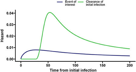
Figure 3. Baseline hazards for the event of interest (blue) and clearance of the initial infection without the event of interest (green) with the dashed vertical lines indicating the time associated with the peak hazard for the event of interest and clearance, respectively.

3.2.2. Simulation scenarios

We simulated data under five different scenarios with a binary covariate (simulated for each individual from a Bernoulli distribution with probability 0.5) defined with effects β₁ = 0.1 and β₂ = −0.3 on the hazards of the event of interest and the competing event, respectively. The simulation scenarios varied in terms of the interval width during follow-up, the distribution of the start time in the origin event interval, the sample size and the maximum time of follow-up.

1. n = 200, 28 day intervals, a maximum follow-up time of 200 days and origin event times that are uniformly distributed in the origin interval.

2. n = 200, 14 day intervals, a maximum follow-up time of 200 days and origin event times that are uniformly distributed in the origin interval.

3. n = 200, 28 day intervals, a maximum follow-up time of 200 days and origin event times that are not uniformly distributed in the origin interval.

4. n = 100, 28 day intervals, a maximum follow-up time of 200 days and origin event times that are uniformly distributed in the origin interval.

5. n = 200, 28 day intervals, a maximum follow-up time of 82 days and origin event times that are uniformly distributed in the origin interval.

3.2.3. Algorithm for simulating double-interval-censored data

We first used the algorithm illustrated by Beyersmann [44] to simulate exact time competing risks data (described in the Supplementary material) with one binary covariate x_i simulated for each individual from a Bernoulli distribution with probability 0.5 and time t_i as the exact survival time (i.e., time to either the event of interest (event 1), competing event (event 2), or right-censored time). Here event/censoring indicators δ_1i and δ_2i were then generated (δ_1i and δ_2i were defined in Section 2.5).

To transform the simulated data into double-interval-censored data, we utilized the following steps. For individual i

1. We defined t_0i: = 0.

2. We defined a sequence of regular follow-up visit times as v_0i = 0, v_ji = jz+e_ji for j = 1, …, m, where z is a fixed width of the follow-up visits, with e_ji~N(0, 3) some noise and m is large enough to include all possible survival times. This results in intervals of (0, v_1i), (v_1i, v_2i), …, (v_{m−1, i}, v_mi) for which the origin and events can occur.

3. The right boundary of the origin event was defined as t_1i = v_1i.

4. We simulated the exact origin time w_i (see Figure 2) from a Uniform distribution between (0, v_1i].

5. The exact event time (or right-censoring time) was calculated as u_i = w_i+t_i.

6. For δ_1i = 1 or δ_2i = 1, the event interval was defined as (t_2i, t_3i) = (v_{j−1, i}, v_ji) if u_i⊂(v_{j−1, i}, v_ji]. For δ_1i = 0 and δ_2i = 0, the event interval was defined as (t_2i, t_3i) = (v_{j−1, i}, ∞) if u_i⊂(v_{j−1, i}, v_ji).

For simulating scenario 3 in Section 3.2.2, we simulated data such that the origin time w_i was not uniformly distributed within (0, v_1i). Here we used an absolute value function of the normal distribution to get some skewness.

3.3. Analysis and performance measures

For every scenario we simulated N = 500 datasets and fitted three models based on each dataset: (1) an exponential PH model; (2) a Weibull PH model; and (3) a B-spline PH model with m₁ = m₂ = 10 basis functions for the event of interest and the competing/clearance event. Convergence in the algorithm is reached when the tolerance (i.e., the difference in parameter estimates between two consecutive iterations) is <1 × 10⁻⁴ or after a maximum of 30 iterations. Moreover, the data with the exact time-to-event (non-interval-censored) data are analyzed with a CPH model. The estimates found from the latter analyses are seen as the best possible results and used for comparison. We will simply refer to these models as the exponential, Weibull, spline, and CPH model.

For all scenarios the performance of each model across simulations are summarized in Table 1. The table gives the bias $(\widehat{\beta }-\beta )$, the empirical standard error (EMPSE, which is the standard deviation of the estimated β's across the different simulations), the model averaged standard errors (MODSE, the average of the SE's across simulations), and the % coverage (cov.) of the true β in the 95% confidence intervals for β. For the estimates of the bias, EMPSE, MODSE, and coverage Monte Carlo standard errors are included in Supplementary Table 1. To investigate sensitivity to the number of basis functions m_k, an additional summary was made for the performance measures (with Monte Carlo standard errors in brackets) of a B-spline model with m₁ = m₂ = 20 basis functions for scenario 1 (see Supplementary Table 2).

TABLE 1

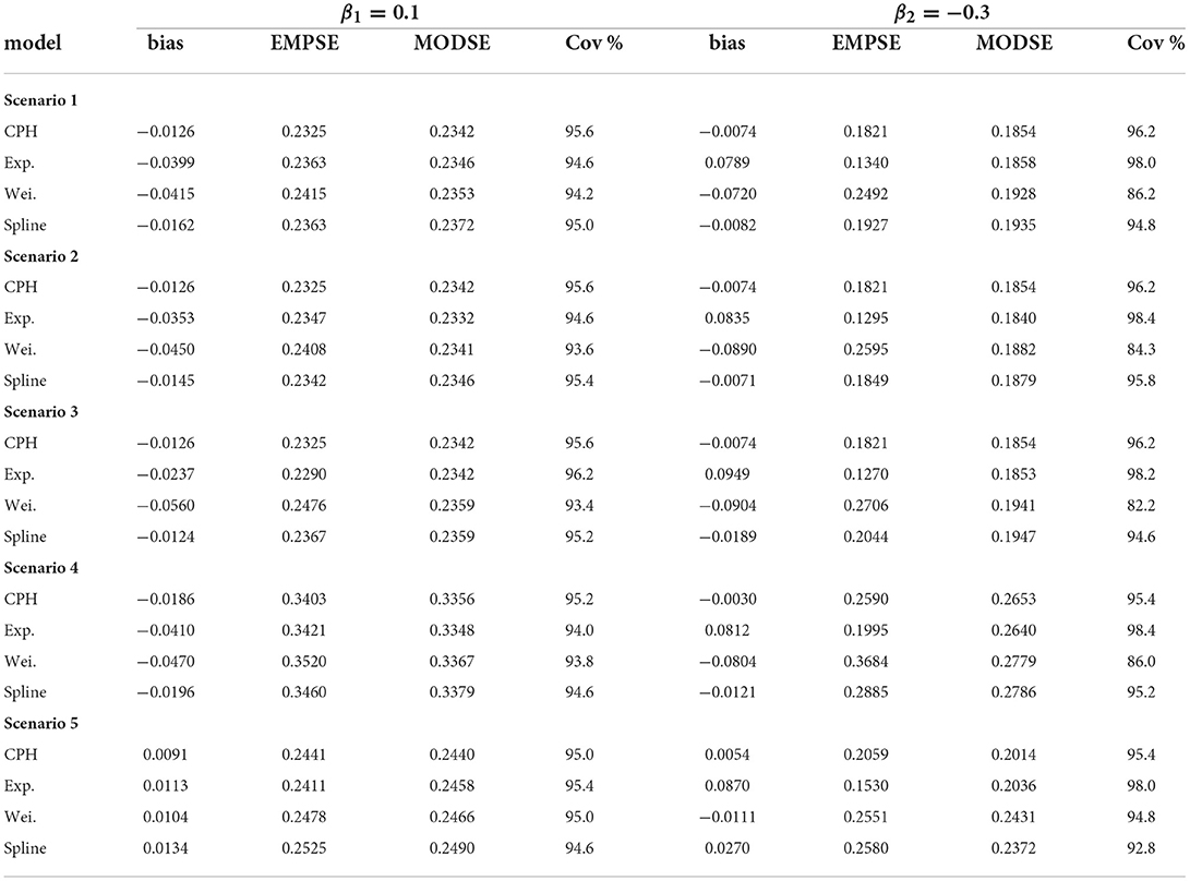
Table 1. Performance measures for all simulation scenarios.

Table 2 shows the estimated mean square error for all estimates from the double-interval-censored model relative to the estimates from the CPH model based on the exact time-to-event data across all simulation scenarios. That is, $cMSE=N^{-1}\sum _{j=1}^N{({\widehat{\beta }}_{j,cph}-{\widehat{\beta }}_{j,model})}^2$ for ${\widehat{\beta }}_{j,cph}$ and ${\widehat{\beta }}_{j,model}$ the estimates in the jth iteration.

TABLE 2

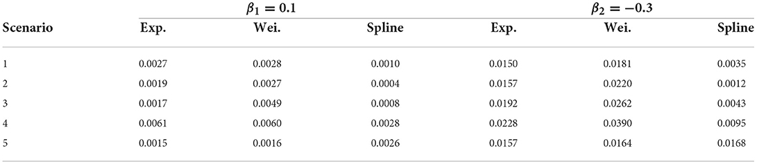
Table 2. Mean square error relative to CPH model estimates.

Two scatter plots are used to summarize the association between the double-interval-censored models and the CPH model in terms of the estimated coefficients (Figure 4) and the estimated standard errors of the coefficients (Figure 5) across simulations for scenario 1. The blue line in each plot is the least squared line and the red line is the y = x line for one-to-one association between the CPH model estimates and the double-interval-censored model estimates. Figures for scenarios 2–5 are included in the Supplementary Figures 1–8. Figure 6 shows the estimated baseline hazards (Figures 6A,C) and cumulative incidence estimates (Figures 6B,D) from the double-interval-censored spline model across simulations for the event of interest (Figures 6A,B) and for the competing event/clearance (Figures 6C,D) in gray relative to the true baseline hazards and cumulative incidences (solid black lines). Figures for scenarios 2–5 are included in the Supplementary Figures 9–12. An additional plot was made for the hazards and cumulative incidence estimates for the B-spline model with m_k = 20 basis functions for each event k = 1, 2 for scenario 1 (see Supplementary Figure 13).

FIGURE 4

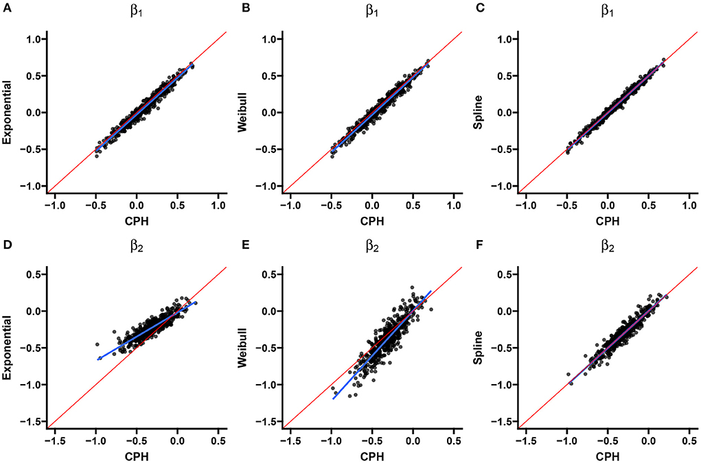
Figure 4. Scenario 1: Correlation with CPH estimates. Scatterplots show the correlation between estimates from the exponential (A,D), Weibull (B,E), and spline models (C,F) for the event of interest (A–C) and the competing/clearance event (D–F) with estimates from the CPH model using exact time data. The blue line is the simple regression line and the red line is the identity line.

FIGURE 5

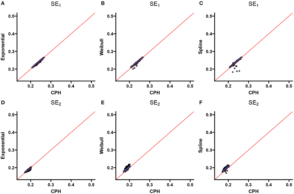
Figure 5. Scenario 1: Correlation with CPH standard errors. Scatterplots show the correlation between standard error estimates from the exponential (A,D), Weibull (B,E), and spline models (C,F) for the event of interest (A–C) and the competing/clearance event (D–F) with standard error estimates from the CPH model using exact time data. The blue line is the simple regression line and the red line is the identity line.

FIGURE 6

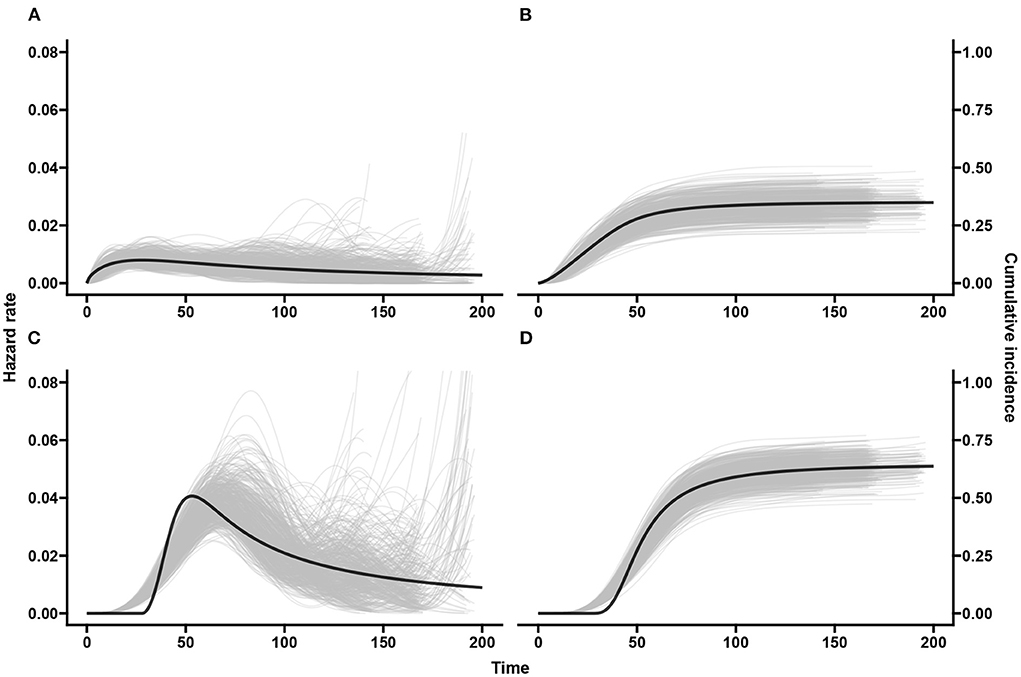
Figure 6. Scenario 1: Baseline hazards and cumulative incidences across simulations. The black line shows the true hazards (A,C) and true cumulative incidences (B,D) for the event of interest (A,B) and competing/clearance event (C,D). The gray curves show estimates from our spline based model applied on the doubly-interval-censored data for all 500 simulated datasets.

3.3.1. Results

For scenarios 1–3, on average, 2.1% of observations across the simulated data was right-censored, 37.8% had experienced the event of interest, and 60.1% had experienced the competing event (i.e., clearance) first. Scenario 4 had an approximately equivalent event proportions. Induced by a shorter follow-up time in scenario 5 there was, on average, 14.8% censored observations, 34.6% with the event of interest, and 50.6% with the competing event/clearance.

In general, across simulation scenarios, there was a little more bias relative to the true effect (β₁ = 0.1) for event of interest compared with the competing event with larger standard errors. The larger standard errors could be attributed to the smaller number of events (a third of the data) for the first event compared with the competing event (more than half the data). The bias is smaller for the spline and CPH models compared with the exponential and Weibull models (see Table 1). The additional bias for the exponential and Weibull models could be explained by the hazard for the event of interest not being entirely flat and not monotonic. Alternatively it could be because of the bias from the mis-specification of the hazards in the competing event. The contribution to the likelihood for the event of interest is a function of the hazard function λ₁(t|x) and survival function S(t) = exp[−Λ₁(t|x)−Λ₂(t|x)]. If λ₂(t|x) is misspecified, it will also have consequences on the likelihood contribution of the first event.

The exponential model tends to underestimate the magnitude of effects (Table 1), much more so for the competing-event with the unimodal hazard than with the even-of-interest with the flatter hazard. This is also the case when comparing individual simulation estimates from the exponential model with the CPH model using exact times (Figure 4). The standard errors closely align with those of the CPH model (Figure 5). For the competing event (with a stronger peak), the empirical standard errors however are much smaller for the model averaged standard errors in all scenarios (Table 1). This could be indicative of an under-fitting model for the competing event.

For the Weibull model from Table 1 it can be seen that the estimated effects are underestimated for the event of interest and show large overestimation for the competing event for all scenarios except for scenario 5 (more right-censoring). While the empirical standard errors and model averaged standard errors do not differ much for the event of interest, we see much larger empirical standard errors for the competing event (with the exception of scenario 5), and lower coverage of the 95% confidence intervals. Except for scenario 5, the Weibull estimates show the largest deviation from the CPH model estimates (Table 2). These findings are confirmed visually for scenarios 1 in Figures 4, 5, and for scenarios 1–4 in the Supplementary material. More right-censoring induced by a shorter follow-up time allows for a more monotonic shape of the hazards to be observed (missing a distinct peak, see Supplementary Figure 12), and could be an explanation of the good performance for the Weibull model under higher right-censoring in this scenario.

Overall, estimated coefficients from the spline model are relatively unbiased (Table 1). The estimated coefficients and standard errors correspond nearly perfectly with the estimates from the CPH model (Figures 4, 5). This is only slightly worse for smaller sample sizes and if the true start times are not uniformly distributed within the start interval, i.e., scenarios 2 and 3. For these scenarios the estimated coefficients themselves however were closer to estimates from the CPH model than the exponential or Weibull models (Table 2).

Studies with smaller sample sizes occur frequently when the prevalence of the infection is low. To determine whether a stricter convergence criteria can improve the fit of the spline model for scenario 4, we re-ran the model with a tolerance of <1 × 10⁻⁵ and a maximum of 50 iterations for convergence. The bias in the coefficient for the competing event reduced from −0.0121 (Table 1) to −0.0081 (Supplementary Table 2) with slightly lower standard errors and slightly higher coverage. The difference was negligible and even more so for the event of interest. We did not repeat this for all scenarios since the stricter convergence criteria makes the computation time of the analysis of the simulated data much longer.

For scenario 2 (shorter follow-up intervals of 14 days) compared with scenario 1 (28 day intervals)) the spline model improves but the exponential and Weibull models perform slightly worse. This may be because there is less uncertainty in the data and thus stronger support that the baseline hazards are misspecified.

Figure 6 middle panel shows that the spline model for double-interval-censoring produces reasonable estimates of the hazard rates. It is also seen that there are higher hazard rates at the tail ends for some of the simulated data-sets. This is not of too much concern as the hazards are conditional probabilities and this means that the few individuals that “survived” until that time experienced the event of interest late. The peak hazard rate is a little shifted toward the right. This was also observed by Machado et al. [32] and was explained by the placement of the knots (we used automatic placement based on percentiles). In Supplementary Figure 13, we use m_k = 20, k = 1, 2 basis functions and we see a much better estimation of the peak hazard but more “wiggliness.” The estimated delayed peak in our spline model with m_k = 10 has a negligible effect on the cumulative incidence and certainly not in the estimated covariate effects.

In summary, to address the aims of the simulation study:

(1) Mis-specifying the baseline hazards was investigated by using an exponential or Weibull model when the hazards (for the competing event) was unimodal. The exponential model underestimated the magnitude of the covariate effect while the Weibull model overstated the effect.

(2) The hazards for the event of interest was “flatter” and we saw that the Weibull and exponential models still showed larger relative bias compared with the spline model. The estimated covariate effects could have been influenced by the bias in the covariate effects on the competing event.

(3) We saw that the estimated covariate effects for the “flatter” event of interested across simulations for all models were closely correlated with those from the CPH model using exact time data. For the unimodal competing event, the exponential model estimates across simulations were much closer to a null effect compared with the CPH model, while the magnitude of the Weibull estimates were larger except for the last scenario. Estimates from the spline model showed nearly perfect one-to-one association with the CPH model.

4. Motivating example

4.1. Background

Malaria transmission epidemiology is used as an illustrative application for the models presented in Section 2. Malaria parasite life cycle involves two hosts: humans and mosquitos. Transmission from infected humans to mosquitoes begins when a subset of asexual parasites converts to female and male gametocytes. Through a blood meal, male and female gametocytes are ingested by anopheles mosquitos. Inside the mosquito parasites fuse, progress through several developmental stages until they multiply and develop into sporozoites. Once sporogenic development is complete, a mosquito becomes infectious and can infect more human hosts through a blood meal. Gametocyte density is a known driver of infectivity in P. falciparum mosquitos [45–47]. Their impact on mosquitoes infectivity was shown by feeding Anopheles coluzzi mosquitoes with natural P. falciparum gametocytes diluted samples [48].

This analysis used malaria incident data obtained from a cohort study conducted in Nagongera subcounty, Tororo district in Eastern Uganda between October 2017 and October 2019. In summary, 531 participants were enrolled from 80 randomly selected households and followed up every 28 days at a designated study clinic [49]. At each follow up, parasite densities were determined microscopically and by ultrasensitive varATS qPCR [50]. All patients that tested positive for microscopy were treated with a 3-day course of artemether-lumefantrine (Coartem, Novartis, Switzerland) while asymptomatic individuals were not treated. Incident malaria infections were estimated based on qPCR negativity. Infections were considered cleared by qPCR if a participant was parasite-free on three consecutive visits. For all qPCR positive samples, female (CCp4 mRNA transcripts) and male (PfMGET mRNA 229 transcripts) gametocyte densities were quantified by quantitative reverse transcriptase PCR [51]. At enrollment, whole blood was also collected to assess host genetic polymorphisms of the HBB gene [52], which is known to have a protective effect against the severe clinical consequences of infection [53, 54] and might also influence gametocytes [55]. Multiplicity of infection (MOI), the number of genetically distinct parasite strains co-infecting a single host, was assessed by apical membrane antigen-1(AMA-1) amplicon deep sequencing [56].

An incident infection was defined as a new malaria infection detected in an individual who was parasite-free by qPCR on three previous visits. Some follow-up times were significantly shorter if participants experienced clinical symptoms and received treatment. Since treatment interrupts the parasite transmission mechanism, we treated the moment of clinical symptoms prior to gametocyte production (if any) as a malaria clearance.

Here, we are interested in the evolution of the hazard rates for the initiation of gametocyte production over time since incident malaria infection, and factors that have a multiplicative effect on this hazard rate. Specifically, we assess the effects of host and parasite characteristics such as age at detected malaria infection (<5 years, 5–15 years, 16+ years), sex, parasite density (log10 transformed), sickle hemoglobin gene (HbS) (HbAA—wildtype HbS, HbSS—sickle cell anemia polymorphism, and HbAS—the human sickle trait polymorphism) and MOI (either single clone or multiclonal). Because of the routinely measured data collection criteria, the time of 104 incident malaria infections are interval-censored and thus the time to initiation of gametocyte production or malaria clearance are double-interval-censored. We also assume that an incident infection could not occur and sporadically clear within the 28 day window. Six individuals in the study had two incident infections each and some infections come from unique individuals in the same household. We do not adjust for this and assume independence between the time-to-event data between incident infections.

From an overview of the data it was clear that many incident infections cleared without first initiating gametocyte production. A competing risk model realizes that malaria clearance prior to gametocyte initiation impedes the observation of gametocyte initiation.

4.2. Analysis and results

From the 104 incident malaria infections, 32 (31%) initiated gametocyte production, 68 (65%) had cleared their malaria without gametocyte production, and the remaining 4 (4%) were right-censored. Missing data were reported in the HbS gene information (3, 2.9%) and in the MOI data (37, 35.6%) due to sequencing failures. All three infected individuals with missing HbS data had cleared their infection without producing gametocytes. From the 37 infected individuals with sequencing failures for MOI, 34 had cleared their infection without gametocytes, 1 had initiated gametocyte production, and 2 were right-censored.

We first estimated the baseline hazards using the exponential, Weibull and spline models without any covariates and then performed univariable analysis with each of the five factors. In Figure 7, the estimated baseline hazards and cumulative incidences are shown. While we see that the shape of the hazards (Figures 7A–C) largely differ between models, the cumulative incidences (Figures 7D–F) are very much similar. From the latter estimates all three models suggest that by 100 days after incident infection approximately one-third of the infections initiate gametocyte production and the remaining two-thirds of infections clear, either naturally or through clinical intervention. Figure 7C suggests that the hazard of gametocyte initiation peaks around three weeks after incident malaria infection and declines rapidly thereafter. This is in line with other findings [57, 58], although they estimated closer to 2 weeks. A later increase in the hazards is also observed for longer event-free infections. In a descriptive analysis, Andolina et al. [59] showed that infection duration was strongly associated with gametocyte initiation. They showed that 82% (18/22) of the long infections (≥12 weeks/84 days) initiated gametocyte production earlier than 12 weeks from detection of incident malaria. From the remaining four infections, three had initiated gametocyte production at or after 12 weeks from detection of incident malaria infections.

FIGURE 7

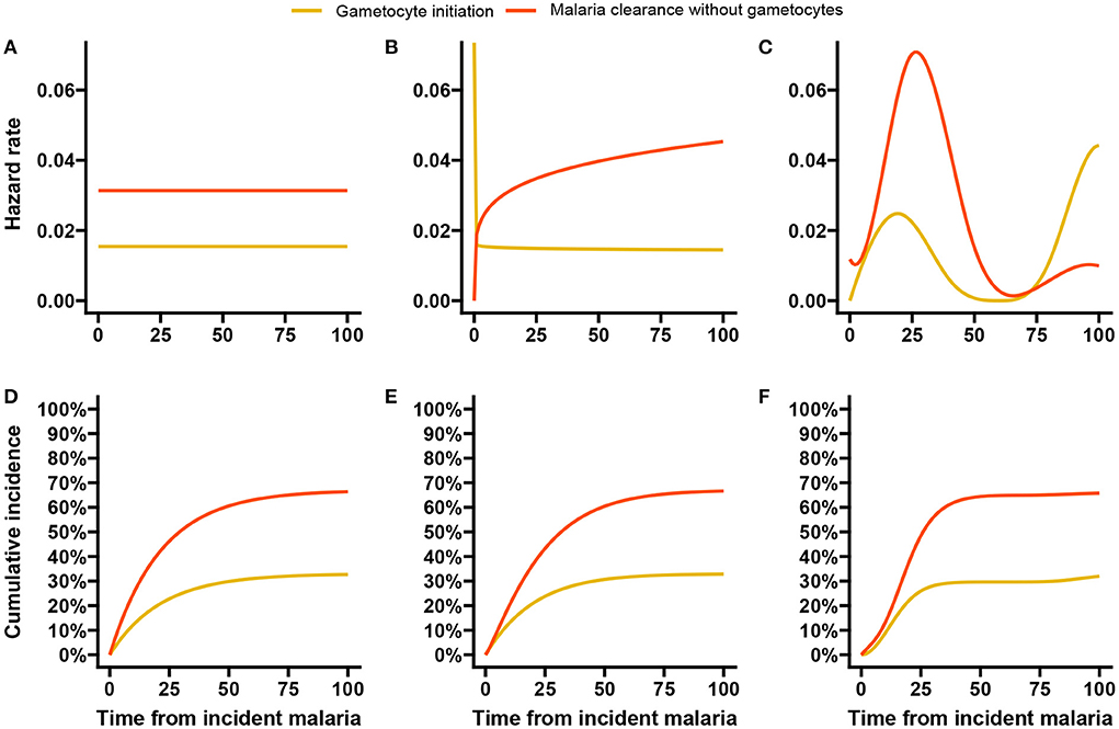
Figure 7. Baseline hazards and cumulative incidences for the malaria data analysis. Here we show the estimated baseline hazards (A–C) and cumulative incidences (D–F) using the exponential, Weibull, and spline baseline proportional hazards models based on double-interval-censored data.

In the simulation study in Section 3, we saw that increasing the number of basis functions improved the estimates of the peak hazards, without much impact on the estimated effects of covariates. We re-ran the malaria data analysis with 15 basis functions for each event and allowed a much larger maximum number of iterations (500) in the estimation algorithm before convergence is reached. The hazards and cumulative incidences are presented in Supplementary Figure 14. Here, we see that the peak hazard for gametocyte initiation is reached at 2 weeks and a slower but steady decline is observed afterwards until the later resurgence. The hazard estimates for malaria clearance without gametocytes remain largely unchanged.

The results of the effects of the covariates are summarized in Table 3. The estimated effects and corresponding p-values (for testing for association) across all models are fairly similar. A significant effect is seen for HbS and parasite density at detection of the initial infection on the initiation of gametocyte production. Specifically, human sickle-cell trait (HbAS) is associated with a nearly three times higher hazard of gametocyte initiation over time compared with wildtype (HbAA). A one unit increase in baseline log parasite density is associated with a nearly 20% increased hazard (p-value <0.001) of gametocyte initiation over time from the spline model. MOI showed a two times hazard of gametocyte initiation for those with more than one co-existing parasite genotype versus those with only one, and this was significant at a 10% level of significance (p-value <0.1) for the exponential and spline models.

TABLE 3

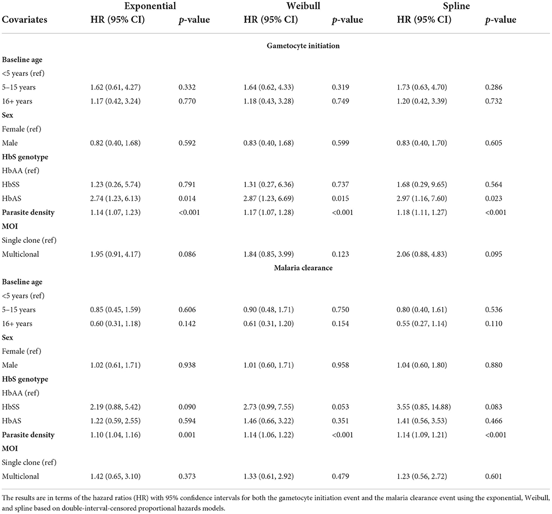
Table 3. Results from the malaria data analysis.

From Table 3, we saw evidence of increased hazards for malaria clearance without gametocytes for higher baseline log parasite densities (HR = 1.14; 95% CI: 1.09–1.21, p-value < 0.001) and HbSS compared with HbAA at the 10% level of significance. Presentation of clinical symptoms was also considered a clearance event, and clinical symptoms are strongly associated with parasite density [60]. When modeling the effect of parasite density for the 88 initially asymptomatic incident infections only, we found no statistically significant effect of baseline parasite density (spline model HR = 1.02; 95% CI 0.93–1.12; p-value = 0.691, see Supplementary Table 3) on malaria clearance without gametocyte production.

5. Discussion and conclusion

In this paper we studied models for double-interval-censored time from infection to event of interest data. Clearance of the infection may prevent the event of interest from happening and, thus, is modeled as a competing risk. We considered models with parametric specifications of the baseline hazards (exponential and Weibull hazards) and a B-spline specification. A penalized likelihood algorithm was used to estimate the parameters for the spline hazards and the penalty factor that controls the smoothness simultaneously. A simulation study was performed to evaluate and compare the model performances for both a flatter and a unimodal baseline hazard. A comparison with the CPH model using the exact times was made as well. An illustrative analysis using malaria data was performed to study the effects of various covariates on the time to gametocyte initiation from incident malaria infection.

In this paper, we focused on clearance of the infection as the competing risk. To be able to observe every infection we had to assume that the infection and its clearance could not happen in the same interval. If an infection would still be observable despite the occurrence of the competing event, this assumption is not necessary. The likelihood function can be simply adjusted: if the i^th individual experienced the competing event in the same interval as the infection, its contribution to the likelihood would be

$\begin{array}{l}{L}_i=\left(\frac{1}{t_i}\right){\displaystyle {\int }_0^{t_{1i}}{\displaystyle {\int }_w^{t_{1i}}\exp }}(-{\text{Λ}}_1(u-w)-{\text{Λ}}_2(u-w)){\lambda }_2(u-w)dudw.\hfill \end{array}$

In the malaria illustrative example we assumed that all incident malaria infections were detected, and no infection with spontaneous clearance had occurred within the 28 days between two consecutive routine follow-up visits. Similarly we assumed that gametocyte production subsequently followed by parasite clearance within the 28 day period does not happen. This assumption implies that we do not miss gametocyte production and misclassify the infection as cleared without gametocyte production. While we cannot completely rule out this may have happened, we consider it unlikely since a prolonged plateau of gametocyte density, lasting several weeks, is observed after low parasite densities in controlled infections [58, 61].

For the derivation of the likelihood we also assumed that every individual had an infection only once during the follow-up time and that there is no clustering in the data. These assumptions may be violated in practice. The simplest way is to ignore it and analyze the data as if this is not the case (we ignored “household” in the illustrative example). This will likely have little effect on the estimated effects, but possibly the estimates of the standard errors are slightly too low. Taking into account clustering or recurrent events among individuals is possible by including a random effect in the model or to determine robust variance estimates. In case of a random effects model we have to adapt the likelihood function: we need to integrate out this random effect. This will result in an extra integral and slows down the estimation procedure.

We used the two step approach proposed by Machado et al. [32] (with an adaptation of the first step) to estimate the spline parameters and smoothing penalty factor simultaneously. Other approaches for estimating the penalty factor are possible. Cai and Betensky [24] used penalized splines for hazards regression with interval-censored data. They utilized the link between smoothing splines and random effects, and thus translated the estimation of the smoothing factor to the estimation of a random effect where the reciprocal of the random effect's variance is the smoothing parameter. This has also been seen in work by Wood et al. [62]. In their work on interval-censoring in an illness-death model with penalized splines, Touraine et al. [63] ignored covariate effects and used a grid search method to find the smoothing factor values for all transitions based on an approximation of the leave-one-out log-likelihood score. Using a random effects approach will induce another integration level in the likelihood, making it more complex. While a grid search approach is simple, it is computationally intensive, especially when multiple smoothing parameters are being estimated, as in our case.

Convergence of the iterative algorithm for estimating the parameters in the spline model relies on two factors: the absolute tolerance, i.e., how small the difference in spline parameters between two iterations should be, and the maximum number of iterations allowed. Ideally the maximum number of iterations should be large enough so that convergence is reached. So using a lower tolerance for convergence should coincide with increasing the maximum number of iterations. Using a stricter criteria, however, comes at the cost of a longer computation time. The exponential and Weibull models both converge much faster than the spline model. For example, when fitting the baseline hazards for the malaria data, the exponential model took 7.18 s, the Weibull model took 18.4 s, the spline model with tolerance 1 × 10⁻⁵ and a maximum of 50 iterations took 1.10 min, and lastly the spline model with tolerance 1 × 10⁻⁷ and a maximum of 100 iterations took 15.3 min (without a noticeable difference in the baseline hazards). These computation times are expected to increase with more covariates and a larger sample size.

The exponential and Weibull model performed decently well for the flatter hazard under all scenarios. It is expected that they would perform much better if the hazards were truly flat, which may be an unrealistic expectation, especially for infectious diseases. The Weibull model showed improved performance in scenario 5 (more right-censoring), especially for the competing event, where due to the shorter follow-up, a distinct peak in the true hazards was no longer seen and the hazards appeared more monotonic. Making the Weibull, due to its simplicity, much more attractive in this scenario. In practice however, the shape of the hazards are usually unknown and understanding the shape of the underlying hazards may be one of the research aims. Here, the spline model is useful in estimating the shape of the baseline hazards as well as estimating unbiased effects without unreasonable assumptions of the baseline hazards.

The methods highlighted in this paper along with the R code, provide an efficient tool for estimating hazard curves, cumulative incidences and/or covariate effects for double-interval-censored time-to-event data in the presence of competing risks. We focused on an infectious disease setting in which the origin time is infection and the competing event is the clearance of this infection. The results of the spline based approach closely aligns with that from the CPH model with exact data and are well-suited to complex forms of the baseline hazards such as unimodal hazards which are prominent in infectious diseases.

Data availability statement

The datasets presented in this study can be found in online repositories. The names of the repository/repositories and accession number(s) can be found at: https://clinepidb.org/ce/app/record/dataset/DS_51b40fe2e2,DS_51b40fe2e2; https://doi.org/10.6084/m9.figshare.20804476.v1; https://figshare.com/articles/dataset/Simulation_results_for_all_scenarios_for_the_analysis_of_double-interval-censored_competing_risks_models/20756668.

Ethics statement

The studies involving human participants were reviewed and approved by the Uganda National Council of Science and Technology (HS119ES), Makerere University School of Medicine, the University of California, San Francisco and the London School of Hygiene & Tropical Medicine. Written informed consent to participate in this study was provided by the participants' legal guardian/next of kin.

Author contributions

JR and MJ contributed to conception and statistical development of the models presented, performed the simulation study, and statistical analysis. TB and CA contributed to the conception, design and data curation for the PRISM2 secondary analysis, from which the ideas for this paper were conceived. JR wrote the first draft of the manuscript. CA wrote a section of the manuscript. MJ and TB supervised the project. All authors contributed to manuscript revision, read, and approved the submitted version.

Funding

JR and TB were supported by the AMMODO science award 2019 awarded to TB. CA and TB were further supported by the European Research Council (grant number ERC-CoG 864180 QUANTUM fellowship to TB) and the National Institutes of Health (grant numbers AI089674 International Centers of Excellence in Malaria Research Program and AI075045).

Acknowledgments

We thank all the study participants for their willingness to support the study, attend the monthly visits and donate blood. We also thank all the lab staff, drivers, and procurement for their dedication in the study. The work presented in this paper is derived from a chapter of the Ph.D. thesis by Ramjith et al. [64].

Conflict of interest

The authors declare that the research was conducted in the absence of any commercial or financial relationships that could be construed as a potential conflict of interest.

Publisher's note

All claims expressed in this article are solely those of the authors and do not necessarily represent those of their affiliated organizations, or those of the publisher, the editors and the reviewers. Any product that may be evaluated in this article, or claim that may be made by its manufacturer, is not guaranteed or endorsed by the publisher.

Supplementary material

The Supplementary Material for this article can be found online at: https://www.frontiersin.org/articles/10.3389/fams.2022.1035393/full#supplementary-material

References

1. Ramjith J, Roes KC, Zar HJ, Jonker MA. Flexible modelling of risk factors on the incidence of pneumonia in young children in South Africa using piece-wise exponential additive mixed modelling. BMC Med Res Methodol. (2021) 21:6. doi: 10.1186/s12874-020-01194-6

PubMed Abstract | CrossRef Full Text | Google Scholar

2. Nijman G, Wientjes M, Ramjith J, Janssen N, Hoogerwerf J, Abbink E, et al. Risk factors for in-hospital mortality in laboratory-confirmed COVID-19 patients in the Netherlands: a competing risk survival analysis. PLoS ONE. (2021) 16:e0249231. doi: 10.1371/journal.pone.0249231

PubMed Abstract | CrossRef Full Text | Google Scholar

3. Sissoko MS, Healy SA, Katile A, Zaidi I, Hu Z, Kamate B, et al. Safety and efficacy of a three-dose regimen of Plasmodium falciparum sporozoite vaccine in adults during an intense malaria transmission season in Mali: a randomised, controlled phase 1 trial. Lancet Infect Dis. (2022) 22:377–89. doi: 10.1016/S1473-3099(21)00332-7

PubMed Abstract | CrossRef Full Text | Google Scholar

4. Oneko M, Steinhardt LC, Yego R, Wiegand RE, Swanson PA, Kc N, et al. Safety, immunogenicity and efficacy of PfSPZ vaccine against malaria in infants in western Kenya: a double-blind, randomized, placebo-controlled phase 2 trial. Nat Med. (2021) 27:1636–45. doi: 10.1038/s41591-021-01470-y

PubMed Abstract | CrossRef Full Text | Google Scholar

5. Rezza G. Determinants of progression to AIDS in HIV-infected individuals: an update from the Italian Seroconversion Study. J Acquir Immune Defic Syndr Hum Retrovirol. (1998) 17:S13–6. doi: 10.1097/00042560-199801001-00005

PubMed Abstract | CrossRef Full Text | Google Scholar

6. Sun J. Statistical analysis of doubly interval-censored failure time data. Handb Stat. (2003) 23:105–22. doi: 10.1016/S0169-7161(03)23006-6

CrossRef Full Text | Google Scholar

7. De Gruttola V, Lagakos SW. Analysis of doubly-censored survival data, with application to AIDS. Biometrics. (1989) 45:1–11. doi: 10.2307/2532030

PubMed Abstract | CrossRef Full Text | Google Scholar

8. Zhang W, Zhang Y, Chaloner K, Stapleton JT. Imputation methods for doubly censored HIV data. J Stat Comput Simul. (2009) 79:1245–57. doi: 10.1080/00949650802255618

PubMed Abstract | CrossRef Full Text | Google Scholar

9. Schuster NA, Hoogendijk EO, Kok AA, Twisk JW, Heymans MW. Ignoring competing events in the analysis of survival data may lead to biased results: a nonmathematical illustration of competing risk analysis. J Clin Epidemiol. (2020) 122:42–8. doi: 10.1016/j.jclinepi.2020.03.004

PubMed Abstract | CrossRef Full Text | Google Scholar

10. Andersen PK, Geskus RB, De Witte T, Putter H. Competing risks in epidemiology: possibilities and pitfalls. Int J Epidemiol. (2012) 41:861–70. doi: 10.1093/ije/dyr213

PubMed Abstract | CrossRef Full Text | Google Scholar

11. Adamic PF. Modeling multiple risks in the presence of double censoring. Scand Actuar J. (2010) 2010:68–81. doi: 10.1080/03461230802420603

PubMed Abstract | CrossRef Full Text | Google Scholar

12. Sankaran P, Sreedevi E. A proportional hazards model for the analysis of doubly censored competing risks data. Commun Stat Theory Methods. (2016) 45:2975–87. doi: 10.1080/03610926.2014.894064

PubMed Abstract | CrossRef Full Text | Google Scholar

13. Gray RJ. A class of K-sample tests for comparing the cumulative incidence of a competing risk. Ann Stat. (1988) 16:1141–54. doi: 10.1214/aos/1176350951

CrossRef Full Text | Google Scholar

14. Cox DR. Regression models and life-tables. J R Stat Soc Ser B. (1972) 34:187–202. doi: 10.1111/j.2517-6161.1972.tb00899.x

CrossRef Full Text | Google Scholar

15. Bender A, Groll A, Scheipl F. A generalized additive model approach to time-to-event analysis. Stat Model. (2018) 18:299–321. doi: 10.1177/1471082X17748083

PubMed Abstract | CrossRef Full Text | Google Scholar

16. Ramjith J, Bender A, Roes KCB, Jonker MA. Recurrent events analysis with piece-wise exponential additive mixed models. Stat Model. (2022). doi: 10.21203/rs.3.rs-563303/v1 [Epub ahead of print].

PubMed Abstract | CrossRef Full Text | Google Scholar

17. Pan W, Chappell R. Estimation in the Cox proportional hazards model with left-truncated and interval-censored data. Biometrics. (2002) 58:64–70. doi: 10.1111/j.0006-341X.2002.00064.x

PubMed Abstract | CrossRef Full Text | Google Scholar

18. Geskus RB. Cause-specific cumulative incidence estimation and the fine and gray model under both left truncation and right censoring. Biometrics. (2011) 67:39–49. doi: 10.1111/j.1541-0420.2010.01420.x

PubMed Abstract | CrossRef Full Text | Google Scholar

19. Andersen PK, Gill RD. Cox's regression model for counting processes: a large sample study. Ann Stat. (1982) 10:1100–20. doi: 10.1214/aos/1176345976

CrossRef Full Text | Google Scholar

20. Prentice RL, Williams BJ, Peterson AV. On the regression analysis of multivariate failure time data. Biometrika. (1981) 68:373–9. doi: 10.1093/biomet/68.2.373

CrossRef Full Text | Google Scholar

21. Hougaard P. Analysis of Multivariate Survival Data. New York, NY: Springer Science & Business Media (2012).

Google Scholar

22. Ng R, Kornas K, Sutradhar R, Wodchis WP, Rosella LC. The current application of the Royston-Parmar model for prognostic modeling in health research: a scoping review. Diagnost Prognost Res. (2018) 2:1–15. doi: 10.1186/s41512-018-0026-5

PubMed Abstract | CrossRef Full Text | Google Scholar

23. Buja A, Hastie T, Tibshirani R. Linear smoothers and additive models. Ann Stat. (1989) 17:453–510. doi: 10.1214/aos/1176347115

CrossRef Full Text | Google Scholar

24. Cai T, Betensky RA. Hazard regression for interval-censored data with penalized spline. Biometrics. (2003) 59:570–9. doi: 10.1111/1541-0420.00067

PubMed Abstract | CrossRef Full Text | Google Scholar

25. Boor Cd. A Practical Guide to Splines, Revised Edn. New-York, NY: Springer (2001).

Google Scholar

26. Wood SN. Generalized Additive Models: An Introduction With R. New York, NY: CRC Press (2017). doi: 10.1201/9781315370279

CrossRef Full Text | Google Scholar

27. Andersen PK, Abildstrom SZ, Rosthøj S. Competing risks as a multi-state model. Stat Methods Med Res. (2002) 11:203–15. doi: 10.1191/0962280202sm281ra

PubMed Abstract | CrossRef Full Text | Google Scholar

28. Sutradhar R, Barbera L. Multistate models for examining the progression of intermittently measured patient-reported symptoms among patients with cancer: the importance of accounting for interval censoring. J Pain Sympt Manage. (2021) 61:54–62. doi: 10.1016/j.jpainsymman.2020.07.012

PubMed Abstract | CrossRef Full Text | Google Scholar

29. Bogaerts K, Komárek A, Lesaffre E. Survival Analysis With Interval-Censored Data: A Practical Approach With Examples in R, SAS, and BUGS. Boca Raton: Chapman and Hall; CRC Press (2017). doi: 10.1201/9781315116945

CrossRef Full Text | Google Scholar

30. Radke BR. A demonstration of interval-censored survival analysis. Prevent Vet Med. (2003) 59:241–56. doi: 10.1016/S0167-5877(03)00103-X

PubMed Abstract | CrossRef Full Text | Google Scholar

31. Withana Gamage PW, Chaudari M, McMahan CS, Kim EH, Kosorok MR. An extended proportional hazards model for interval-censored data subject to instantaneous failures. Lifetime Data Anal. (2020) 26:158–82. doi: 10.1007/s10985-019-09467-z

PubMed Abstract | CrossRef Full Text | Google Scholar

32. Machado RJ, van den Hout A, Marra G. Penalised maximum likelihood estimation in multi-state models for interval-censored data. Comput Stat Data Anal. (2021) 153:107057. doi: 10.1016/j.csda.2020.107057

CrossRef Full Text | Google Scholar

33. Kim MY, De Gruttola VG, Lagakos SW. Analyzing doubly censored data with covariates, with application to AIDS. Biometrics. (1993) 49:13–22. doi: 10.2307/2532598

PubMed Abstract | CrossRef Full Text | Google Scholar

34. Sun J, Liao Q, Pagano M. Regression analysis of doubly censored failure time data with applications to AIDS studies. Biometrics. (1999) 55:909–14. doi: 10.1111/j.0006-341X.1999.00909.x

PubMed Abstract | CrossRef Full Text | Google Scholar

35. Pan W. A multiple imputation approach to regression analysis for doubly censored data with application to AIDS studies. Biometrics. (2001) 57:1245–50. doi: 10.1111/j.0006-341X.2001.01245.x

PubMed Abstract | CrossRef Full Text | Google Scholar

36. Turnbull BW. The empirical distribution function with arbitrarily grouped, censored and truncated data. J R Stat Soc Ser B. (1976) 38:290–5. doi: 10.1111/j.2517-6161.1976.tb01597.x

CrossRef Full Text | Google Scholar

37. Piessens R, de Doncker-Kapenga E, Überhuber CW, Kahaner DK. Quadpack: A Subroutine Package for Automatic Integration. Vol. 1. Berlin; Heidelberg: Springer Science & Business Media (2012).

Google Scholar

38. Gerber F, Furrer R. optimParallel: An R package providing a parallel version of the L-BFGS-B optimization method. R J. (2019) 11:352–8. doi: 10.32614/RJ-2019-030

CrossRef Full Text | Google Scholar

39. Byrd RH, Lu P, Nocedal J, Zhu C. A limited memory algorithm for bound constrained optimization. SIAM J Sci Comput. (1995) 16:1190–208. doi: 10.1137/0916069

CrossRef Full Text | Google Scholar

40. Marra G, Radice R, Bärnighausen T, Wood SN, McGovern ME. A simultaneous equation approach to estimating HIV prevalence with nonignorable missing responses. J Am Stat Assoc. (2017) 112:484–96. doi: 10.1080/01621459.2016.1224713

CrossRef Full Text | Google Scholar

41. Craven P, Wahba G. Smoothing noisy data with spline functions. Numer Math. (1978) 31:377–403. doi: 10.1007/BF01404567

CrossRef Full Text | Google Scholar

42. Wood SN. Stable and efficient multiple smoothing parameter estimation for generalized additive models. J Am Stat Assoc. (2004) 99:673–86. doi: 10.1198/016214504000000980

CrossRef Full Text | Google Scholar

43. Khan SA, Khosa SK. Generalized log-logistic proportional hazard model with applications in survival analysis. J Stat Distrib Appl. (2016) 3:1–18. doi: 10.1186/s40488-016-0054-z

PubMed Abstract | CrossRef Full Text | Google Scholar

44. Beyersmann J, Latouche A, Buchholz A, Schumacher M. Simulating competing risks data in survival analysis. Stat Med. (2009) 28:956–71. doi: 10.1002/sim.3516

PubMed Abstract | CrossRef Full Text | Google Scholar

45. Schneider P, Bousema JT, Gouagna LC, Otieno S, Van De Vegte-Bolmer M, Omar SA, et al. Submicroscopic Plasmodium falciparum gametocyte densities frequently result in mosquito infection. Am J Trop Med Hyg. (2007) 76:470–4. doi: 10.4269/ajtmh.2007.76.470

PubMed Abstract | CrossRef Full Text | Google Scholar

46. Bradley J, Stone W, Da DF, Morlais I, Dicko A, Cohuet A, et al. Predicting the likelihood and intensity of mosquito infection from sex specific Plasmodium falciparum gametocyte density. Elife. (2018) 7:e34463. doi: 10.7554/eLife.34463.020

PubMed Abstract | CrossRef Full Text | Google Scholar

47. Rek J, Blanken SL, Okoth J, Ayo D, Onyige I, Musasizi E, et al. Asymptomatic school-aged children are important drivers of malaria transmission in a high endemicity setting in Uganda. J Infect Dis. (2022) 226:708–13. doi: 10.1093/infdis/jiac169

PubMed Abstract | CrossRef Full Text | Google Scholar

48. Da DF, Churcher TS, Yerbanga RS, Yaméogo B, Sangaré I, Ouedraogo JB, et al. Experimental study of the relationship between Plasmodium gametocyte density and infection success in mosquitoes; implications for the evaluation of malaria transmission-reducing interventions. Exp Parasitol. (2015) 149:74–83. doi: 10.1016/j.exppara.2014.12.010

PubMed Abstract | CrossRef Full Text | Google Scholar

49. Nankabirwa JI, Arinaitwe E, Rek J, Kilama M, Kizza T, Staedke SG, et al. Malaria transmission, infection, and disease following sustained indoor residual spraying of insecticide in Tororo, Uganda. Am J Trop Med Hyg. (2020) 103:1525. doi: 10.4269/ajtmh.20-0250

PubMed Abstract | CrossRef Full Text | Google Scholar

50. Hofmann N, Mwingira F, Shekalaghe S, Robinson LJ, Mueller I, Felger I. Ultra-sensitive detection of Plasmodium falciparum by amplification of multi-copy subtelomeric targets. PLoS Med. (2015) 12:e1001788. doi: 10.1371/journal.pmed.1001788

PubMed Abstract | CrossRef Full Text | Google Scholar

51. Meerstein-Kessel L, Andolina C, Carrio E, Mahamar A, Sawa P, Diawara H, et al. A multiplex assay for the sensitive detection and quantification of male and female Plasmodium falciparum gametocytes. Malar J. (2018) 17:1–11. doi: 10.1186/s12936-018-2584-y

PubMed Abstract | CrossRef Full Text | Google Scholar

52. Grignard L, Mair C, Curry J, Mahey L, Bastiaens GJ, Tiono AB, et al. Bead-based assays to simultaneously detect multiple human inherited blood disorders associated with malaria. Malar J. (2019) 18:1–9. doi: 10.1186/s12936-019-2648-7

PubMed Abstract | CrossRef Full Text | Google Scholar

53. Aidoo M, Terlouw DJ, Kolczak MS, McElroy PD, Ter Kuile FO, Kariuki S, et al. Protective effects of the sickle cell gene against malaria morbidity and mortality. Lancet. (2002) 359:1311–2. doi: 10.1016/S0140-6736(02)08273-9

PubMed Abstract | CrossRef Full Text | Google Scholar

54. Williams TN, Mwangi TW, Wambua S, Alexander ND, Kortok M, Snow RW, et al. Sickle cell trait and the risk of Plasmodium falciparum malaria and other childhood diseases. J Infect Dis. (2005) 192:178–86. doi: 10.1086/430744

PubMed Abstract | CrossRef Full Text | Google Scholar

55. Gouagna LC, Bancone G, Yao F, Yameogo B, Dabiré KR, Costantini C, et al. Genetic variation in human HBB is associated with Plasmodium falciparum transmission. Nat Genet. (2010) 42:328–31. doi: 10.1038/ng.554

PubMed Abstract | CrossRef Full Text | Google Scholar

56. Briggs J, Teyssier N, Nankabirwa JI, Rek J, Jagannathan P, Arinaitwe E, et al. Sex-based differences in clearance of chronic Plasmodium falciparum infection. Elife. (2020) 9:e59872. doi: 10.7554/eLife.59872.sa2

PubMed Abstract | CrossRef Full Text | Google Scholar

57. Johnston GL, Gething PW, Hay SI, Smith DL, Fidock DA. Modeling within-host effects of drugs on Plasmodium falciparum transmission and prospects for malaria elimination. PLoS Comput Biol. (2014) 10:e1003434. doi: 10.1371/journal.pcbi.1003434

PubMed Abstract | CrossRef Full Text | Google Scholar

58. Reuling IJ, Van De Schans LA, Coffeng LE, Lanke K, Meerstein-Kessel L, Graumans W, et al. A randomized feasibility trial comparing four antimalarial drug regimens to induce Plasmodium falciparum gametocytemia in the controlled human malaria infection model. Elife. (2018) 7:e31549. doi: 10.7554/eLife.31549

PubMed Abstract | CrossRef Full Text | Google Scholar

59. Andolina C, Ramjith J, Rek J, Lanke K, Okoth J, Grignard L, et al. Gametocyte production in incident P. falciparum infections: a longitudinal study in a low transmission setting under intensive vector control. medRxiv [Pre-print]. (2022). doi: 10.1101/2022.08.29.22279332

CrossRef Full Text | Google Scholar

60. Andolina C, Rek JC, Briggs J, Okoth J, Musiime A, Ramjith J, et al. Sources of persistent malaria transmission in a setting with effective malaria control in eastern Uganda: a longitudinal, observational cohort study. Lancet Infect Dis. (2021) 21:1568–78. doi: 10.1016/S1473-3099(21)00072-4

PubMed Abstract | CrossRef Full Text | Google Scholar

61. Collins KA, Wang CY, Adams M, Mitchell H, Rampton M, Elliott S, et al. A controlled human malaria infection model enabling evaluation of transmission-blocking interventions. J Clin Invest. (2018) 128:1551–62. doi: 10.1172/JCI98012

PubMed Abstract | CrossRef Full Text | Google Scholar

62. Wood SN, Pya N, Säfken B. Smoothing parameter and model selection for general smooth models. J Am Stat Assoc. (2016) 111:1548–63. doi: 10.1080/01621459.2016.1180986

CrossRef Full Text | Google Scholar

63. Touraine C, Gerds TA, Joly P. SmoothHazard: An R package for fitting regression models to interval-censored observations of illness-death models. J Stat Softw. (2017) 79:1–22. doi: 10.18637/jss.v079.i07

CrossRef Full Text | Google Scholar

64. Ramjith J. Flexible Time-to-Event Models for Complex Infectious Disease Data. Nijmegen: Radboud University Medical Center (2022).

Google Scholar