The hybrid model of autoregressive integrated moving average and fuzzy time series Markov chain on long-memory data

1. Introduction

Crude oil is a commodity that plays an essential role in the economy. Fluctuations in crude oil prices can impact the health of the world economy, especially in crude oil-producing countries. This condition occurs because countries that import crude oil are more susceptible to price changes with transactions carried out in US dollars (USD). One of the crude oil types used as a benchmark in determining oil prices is West Texas Intermediate (WTI). WTI oil, according to the U.S. Energy Information Administration (EIA) website, is included as a type of petroleum that is low in density. WTI oil contains about 0.24% sulfur and a gravity of 39.6°. This oil is usually considered of good quality for processing into gasoline. Therefore, this high-quality WTI oil is used as the standard price for world oil.

The fluctuation of crude oil prices shows a pattern and identifies the component factors that influence it in the short and long term. The classical time series model of autoregressive integrated moving average (ARIMA) is often used to produce accurate short memory modeling [1]. In nonlinear time series data, the accuracy of the ARIMA model in forecasting is quite good than the recurrence quantification analysis (RQA) predictive model [2]. However, the heteroscedasticity in the ARIMA model can be corrected by using a variance model, that is the GARCH model [3] or the GARCH exponential [4] or the mixed memory MMGARCH [5].

Oil price movements are very volatile and tend to be affected for a long time. Thus, there are some cases of time-series data showing a long-memory pattern. In brain stimulation, for instance, this volatility problem as the dynamical pattern is extended through stimulation for long-term targeting and control of post-stimulation [6]. This long-memory case is characterized by decaying correlation slowly over time at infinity [7]. As a result, the value of the differentiating coefficient in the form of an integer number cannot provide an accurate estimate in the ARIMA model, so the fractional differentiating number of the ARFIMA model is used instead [8]. The method for estimating the value of the fractional differentiating coefficient in the ARFIMA model that is often used is the Geweke and Porter-Hudak (GPH) method to estimate the differentiating coefficient parameter directly without knowing the value of the autoregressive (AR) or the moving average (MA) order [9]. In addition, the Whittle estimator is provided for obtaining the parameter estimates for the stationary time series model of ARMA and ARFIMA, which is the basis of the Jackknifed empirical likelihood inference [10].

Classical time series data modeling require many assumptions. Thus, many have developed time-series data modeling using a fuzzy logic approach, the fuzzy time series (FTS) method. The simple arithmetic operations on time series data were applied to develop the early period of FTS, while a fuzzy logic was proposed by using weighting and adaptive modeling [11]. Finally, the FTS model has been applied in forecasting oil production and consumption [12]. Further developments in 2012, the fuzzy time series Markov chain (FTSMC) was first proposed as a new concept to analyze the accuracy of currency exchange rate predictions. This FTSMC method gives quite good results compared to the FTS method [13]. Furthermore, the forecasting method of FTSMC was also carried out on gold prices as the investment information [14]. In addition, three FTS methods, namely FTS Chen, FTS Segmented Chen, and FTSMC are compared to forecast bitcoin prices [2]. Based on the mean absolute percentage error (MAPE) accuracy value, the FTSMC method still gave better results. These results confirmed that the FTSMC method provides a pretty good modeling accuracy than other FTS methods.

Time series data modeling with FTS has many parameters because the model changes in each iteration process. A simple structure has been proposed to overcome this model change. Parsimony FTS is used in forecasting prices for liquid bulk cargo carriers and secondhand ships [15]. In advanced financial cases, the time series data of the Indonesian Composite index price was analyzed by using the nonlinear artificial intelligence method, which produced the best accuracy based on the MAPE value [16]. Meanwhile, a development of the hybrid ARIMA model and a wavelet-based artificial intelligence model gave more accurate results than the ARIMA model or artificial intelligence model [17]. However, ARIMA, ARFIMA, and FTS models have something in common: using past values to produce modeling in the future period. The difference is in the residual assumption test that must be met using the classical ARIMA and ARFIMA models. These assumptions are not a concern for modeling with the FTS method. Meanwhile, the residual of model ARIMA and ARFIMA can be adjusted in their value and residual assumptions by combining the model of ARIMA and ARFIMA with the numerical data processing of the fuzzy time series Markov chain. This study proposes the best modeling for West Texas Intermediate (WTI) crude oil prices using the hybrid model of ARIMA-FTSMC and the hybrid model of ARFIMA-FTSMC hybrid models, compared to the classical ARIMA and ARFIMA models based on the level of accuracy measured using mean absolute percentage error (MAPE), mean absolute error (MAE), and root mean square error (RMSE).

2. Materials and methods

This study uses available data from West Texas Intermediate Oil (WTI) on the U.S. Energy Information Administration (EIA) website with the monthly period during the 2003–2021 time period, consisting of 18 years selected as many as 217 data. The time series data used are long-memory which will be modeled into classical time series models and hybrid models. Furthermore, in this section, theories and processes related to the formation of target models will be explained, namely the model of ARIMA, the model of ARFIMA, the hybrid model of ARIMA-FTSMC, and the hybrid model of ARFIMA-FTSMC.

2.1. Autoregressive integrated moving average

A time series {X_t} has the properties of white noise if a sequence of uncorrelated random variables with a specific distribution is identified by constant mean, usually assumed to be 0, a constant variance $Var(X_t)={\sigma }^2$ and Cov(X_t+h, X_t) = 0 for k≠0. In time series analysis, there are some time series models such as ARIMA which is a combined two models between autoregressive (AR) and moving average (MA) after differencing. The common form of the ARIMA model is expressed as follows:

$\begin{array}{ll}{\varphi }_p(B){(1-B)}^d{X}_t={\theta }_q(B){\epsilon }_t& (1)\end{array}$

with

$\begin{array}{lll}{\varphi }_p(B)& =& (1-{\varphi }_{1}B-{\varphi }_2{B}^2-\cdots -{\varphi }_p{B}^p)\\ {\theta }_q(B)& =& (1-{\theta }_{1}B-{\theta }_2{B}^2-\cdots -{\theta }_q{B}^q)\end{array}$

where ϕ_p(B) is the autoregressive components, θ_q(B) is the moving average components, B is the operator of backward shift, and ${(1-B)}^d{X}_t$ is stationary of time series in d-order differencing. This process is denoted by ARIMA(p,d,q).

For detecting the stationarity of data, graph analysis can not be proposed to determine whether the time series data are already stationary, but it helps to know how the pattern of the data. The basic properties are still needed to determine the next decision. If the data have a constant mean and variance, the data are already stationary. If the variance of the data is non-stationary, it can be solved by using the power transformation, namely the Box–Cox transformation. Let T(X_t) be the transformation function of X_t. The following formula is used to stabilize the variance

$\begin{array}{ll}T(X_t)=\frac{X_t^{\lambda }-1}{\lambda }& (2)\end{array}$

for λ≠0 and λ called transformation parameter. After the data are stationary in variance, it is followed by testing the stationary in the mean by using augmented Dickey–Fuller (ADF) test. The random walk equation with drift for the differenced-lag model is regressed to be:

$\begin{array}{ll}\nabla X_t=\mu +\delta X_{t-1}+{\displaystyle \sum _{i=1}^k}{\varphi }_i\nabla X_{t-i}+e_t& (3)\end{array}$

for ∇X_t = X_t−X_t−1, k is the number of lags, δ is the slope coefficient, μ is a drift parameter, ϕ_i is the parameter of random walk equation, and e_t is the white noise error term. The test statistic is used as follows:

$\begin{array}{ll}ADF=\frac{\widehat{\delta }}{SE(\widehat{\delta })}& (4)\end{array}$

for $\widehat{\delta }$ as the estimated δ which is obtained by using ordinary least squares and $SE(\widehat{\delta })$ as the standard error of δ. The initial or null hypothesis of δ = 0 means that the stationarity has not been fulfilled. The conclusion of the ADF hypothesis test is rejecting the null hypothesis if the ADF value is less than the test statistics.

The model of autoregressive integrated moving average (ARIMA) can be built by using the following steps.

1. Checking the stationarity of the data against the variance with Box–Cox transformation and the stationarity of the mean value by differencing and augmented Dickey–Fuller (ADF) test.

2. Identifying possible ARIMA models by determining orders based on lag correlation analysis on ACF and Partial ACF (PACF) plots.

3. Estimating significance parameter on ARIMA model with significant level α = 5%.

4. Choosing the best ARIMA model that has the smallest value of Akaike Information Criterion (AIC) and Bayesian Information Criterion (BIC) values using the formulation below

$\begin{array}{llll}AIC& =& nln({\widehat{{\sigma }_{\epsilon }}}^2)+2k& (5)\end{array}$

$\begin{array}{llll}BIC& =& nln({\widehat{{\sigma }_{\epsilon }}}^2)+kln(n)& (6)\end{array}$

for n is the number of observations, ${\widehat{\sigma }}_{\epsilon }^2$ is the maximum likelihood estimator of ${\sigma }_{\epsilon }^2$, and k is the number of parameters estimated.

5. Testing the ARIMA model residual assumptions using non-autocorrelation, homoscedasticity, and normality tests.

a. Non-autocorrelation test using QLjung-Box test with the equation:

$\begin{array}{ll}{Q}_{LB}=n(n+2){\displaystyle \sum _{i=1}^k}\frac{{\rho }_i^2}{n-i}& (7)\end{array}$

where k is the number of lag, n is the number of observations, and ${\rho }_i^2$ is the autocorrelation of the i-th residual for i = 1, 2, …, k. The value of Q_LB follows χ² distribution with a degree of freedom k−p−q where p and q are the order in the ARIMA model. If $Q_{LB}<{\chi }_{\alpha }^2(k-p-q)$, then the residual in the model is non-autocorrelation.

b. The homoscedasticity test was carried out using the Lagrange multiplier test with the test statistic,

$\begin{array}{ll}LM=n{R}^2& (8)\end{array}$

where n is the number of observations and R² is the coefficient of determination of the quadratic residual regression model. The LM value follows χ² distribution with a degree of freedom q which is one order in the ARIMA model. If $LM<{\chi }_{\alpha }^2(q)$, then the residual in the model is homoscedasticity.

c. The normality test was carried out using the Jarque–Bera hypothesis with the test statistic

$\begin{array}{ll}JB=\frac{n}{6}(S^2+\frac{{(K-3)}^2}{4})& (9)\end{array}$

where n is the number of observations,

$\begin{array}{l}S=\frac{\frac{1}{n}{\left({\epsilon }_i-\overline{\epsilon }\right)}^3}{{\left(\frac{1}{n}{\displaystyle {\sum }_{i=1}^n{({\epsilon }_i-\overline{\epsilon })}^2}\right)}^{\frac{3}{2}}}K=\frac{\frac{1}{n}{({\epsilon }_i-\overline{\epsilon })}^4}{{\left(\frac{1}{n}{\displaystyle {\sum }_{i=1}^n{({\epsilon }_i-\overline{\epsilon })}^2}\right)}^2},\\ \text{and }\overline{\epsilon }=\frac{{\displaystyle {\sum }_{i=1}^n{\epsilon }_i}}{n}\end{array}$

The JB value follows χ² distribution with a degree of freedom of 2. If the $JB<{\chi }_{\alpha }^2(2)$, then the residual in the model is normally distributed.

2.2. Autoregressive fractional integrated moving average

Autoregressive fractionally integrated moving average (ARFIMA) was first introduced by Grager and Joyeux in 1980 which is the development of the autoregressive integrated moving average (ARIMA) model to model long-term data. Long memory is a stationary time series that has a long-term dependence between observations with periods that are far apart but still have a high correlation. This can also be seen from the autocorrelation function that decays slowly over a long period. The ARFIMA(p, d, q) model, where p and q are non-negative integers and d is a real number in the interval 0 < d < 0.5. The general model ARFIMA(p, d, q) can be shown as follows Wei WWS [1]:

$\begin{array}{ll}{\varphi }_p(B){(1-B)}^d{X}_t={\theta }_q(B){\epsilon }_t& (10)\end{array}$

where ${\varphi }_p(B)=(1-{\varphi }_{1}B-{\varphi }_2{B}^2-...-{\varphi }_p{B}^p)$, ${\theta }_q(B)=(1-{\theta }_{1}B-{\theta }_2{B}^2-...-{\theta }_q{B}^q)$, B as backshift operator, d as the differencing in real number, ${(1-B)}^d{X}_t$ as the time series that has been already at differencing, θ_i as the parameter of MA for i, i = 1, 2, …, q, ϕ_i as the parameter of AR for i, i, 1, 2, …, p, and ${\epsilon }_t~WN(0,{\sigma }^2)$.

The model building of the autoregressive fractional integrated moving average (ARFIMA) can be determined by using the following steps.

1. Checking the stationary of the data against variance. If the data are not stationary concerning variance, a transformation is carried out using the Box–Cox transformation method to obtain a rounded value (λ).

2. Checking the stationary of the data in the mean using augmented Dickey–Fuller (ADF). If the data are not stationary concerning the mean, then a differencing is required.

3. Estimating differencing parameters using the GPH method with the following formula:

$\begin{array}{ll}{\hat{d}}_{GPH}=\frac{{\displaystyle \sum _{j=1}^m}(x_j-\overline{x})(y_j-\overline{y})}{{\displaystyle \sum _{j=1}^m}{(x_j-\overline{x})}^2}.& (11)\end{array}$

where y_j = lnI(λ_j) and $x_j=-ln{(2sin(\frac{{\lambda }_j}{2}))}^2$. The I(λ_j) function is a periodogram with a frequency of Fourier ${\lambda }_j=\frac{2\pi j}{T}$, j = 1, 2, …, m, and T is the number of observation data, while m is the limit of the number of Fourier frequencies.

4. Differentiating data that have been transformed using the value of ${\widehat{d}}_{GPH}$.

5. Identifying the ARFIMA model by determining the combination of the ARFIMA model by making ACF and PACF plots from the differencing of data. The ACF plot shows the order of MA(q), and the plot of the PACF shows the order of AR(p).

6. Parameter estimation and significance test of the ARFIMA model have been declared significant if the model parameter's probability value is smaller than α = 5%.

7. Choosing the best ARFIMA model is the model that has the smallest AIC and BIC values.

8. Testing the best ARFIMA model residual assumptions, namely non-autocorrelation, heteroscedasticity, and normality tests.

2.3. Proposed model of hybrid ARIMA-FTSMC

The ARIMA-FTSMC hybrid model is a proposed model by combining the ARIMA model for initial data and the FTSMC model for residual data. The first step is to model the time series data with the best ARIMA model. In improving the ARIMA model, the residual ARIMA model is analyzed by using Geweke and Porter–Hudak (GPH) in Equation (11) to determine whether there still contains long-memory properties. The improvement of the residual ARIMA can apply the FTSMC model as the alternative method because the FTSMC model does not require stationary data and regression assumption. Finally, residual modeling results from the FTSMC model are entered into the ARIMA model to obtain the ARIMA-FTSMC hybrid modeling. The steps for modeling ARIMA residuals using the FTSMC model are as follows:

1. Definition of the union of sets U. In the first stage, determine the maximum value (D_max) and minimum value (D_min) from ARIMA data residual. Choose any positive value for D₁ and D₂ so that they can be used in the formation of the union of sets U with the following conditions:

$\begin{array}{ll}U=[D_{min}-D_1,D_{max}+D_2),& (12)\end{array}$

2. Interval formation and interval length. The union of sets U will be partitioned into parts with equal intervals (n). By using the Sturges formula as follows:

$\begin{array}{ll}n=1+3.322logN,& (13)\end{array}$

where N is the number of ARIMA residual data. Here is the formula for determining the length of the interval:

$\begin{array}{ll}l=\frac{\left[(D_{max}+D_2)-(D_{min}-D_1)\right]}{n},& (14)\end{array}$

and l is the length of the interval and n is the number of intervals. Each interval can be calculated as follows:

$\begin{array}{llll}{u}_n& =& [D^{*}+(n-1)l,D^{*}+nl).& (15)\end{array}$

where $D^{*}=D_{min}-D_1$.

3. The definition of fuzzy sets for each interval. If the ARIMA residual data are in the interval u_i, then the fuzzy set of the data is denoted as A_i.

4. Determination of fuzzy logic relations (FLRs). If F(t) = A_i and F(t−1) = A_j, then the relationship between F(t) and F(t−1) is called a fuzzy logical relationship (FLR). This relationship can be expressed by A_i→A_j, where A_i is the left-hand side (LHS) and A_j is the right-hand side (RHS) from FLR.

5. Determination of fuzzy logic relations group (FLRG). If two FLRs have the same fuzzy set (LHS A_i→A_j1, A_i→A_j2), then it can be grouped into fuzzy logical relationship groups (FLRGs) A_i→A_j1, A_j2.

6. Markov transition probability matrix formation.

$\begin{array}{ll}{P}_{ij}=\frac{M_{ij}}{M_i},i,j=1,2,3,...,n,& (16)\end{array}$

Transition probability of state A_i to A_j in one step is P_ij. The number of data from state A_i is M_i. The transition time of state A_i to A_j in one step is M_ij. Transition probability matrix R using n×n dimension can be written as:

$\begin{array}{ll}\text{R}=\left[\begin{array}{cccc}{P}_{11}& P_{12}& \dots & P_{1n}\\ P_{21}& P_{22}& \dots & P_{2n}\\ ⋮& ⋮& \ddots & ⋮\\ P_{n1}& P_{n2}& \dots & P_{nn}\\ & & & \end{array}\right].& (17)\end{array}$

7. Calculation of the initial modeling results based on the transition probability R matrix with the following rules:

a. If FLRG from A_i transitions to the empty set, A_i → ϕ , then the modeling results of F(t) is m_i, where m_i is the median of u_i, with equation:

$\begin{array}{ll}{F}_t=m_i.& (18)\end{array}$

b. If FLRG A_i transitions to, A_i→A_k and P_ik = 1, j≠k, the modeling result of F(t) is m_k as the median of u_k, with equation:

$\begin{array}{ll}{F}_t=m_k{P}_{ik}=m_k.& (19)\end{array}$

c. If FLRG A_j makes a one-to-many transition, A_i→A₁, A₂, …, A_n, j = 1, 2, …, n, and datasets X_t−1 when t−1 is in state A_j, then the modeling results of F(t) are as follow:

$\begin{array}{l}{F}_t=m_1{P}_{j1}+m_2{P}_{j2}+\cdots +m_{j-1}{P}_{j(j-1)}+X_{t-1}{P}_{jj}\\ +m_{j+1}{P}_{j(j+1)}+\cdots +m_{n-1}{P}_{j(n-1)}+m_n{P}_{jn},& (20)\end{array}$

where m₁, m₂, …, m_j−1, m_j+1, …, m_n is the median of u₁, u₂, …, u_j−1, u_j+1, …, u_n. The m_j value was substituted by X_t−1 in order to obtain information from the state A_j when t−1.

8. Calculation of modeling adjustment values that aim to correct modeling errors. This is due to the biased transition probability R matrix. The calculation of the modeling adjustment value is as follows:

a. If state A_i when t−1 as F_t−1 = A_i, and t with equation (1 ≤ s ≤ n−i) there is a forward transition jump to state A_i+s, then D_t as the adjustment value is defined as $D_t=(\frac{l}{2})s$ where 1 ≤ s ≤ n−i, l is the length of the interval, and s is the number of forwarding transition displacement jumps.

b. If state A_i when t−1 as F_t−1 = A_i, and when t as (1 ≤ v ≤ i) there is a transition jump backward transition to state A_i−v, then D_t as the adjustment value is defined as $D_t=-(\frac{l}{2})v$, where 1 ≤ v ≤ i, l is the length of the interval, and v is the number of jumps of the backward transition displacement.

9. Calculation of the final modeling results. The general form of the final modeling result is the form:

$\begin{array}{ll}F{M}_t=F_t+D_t.& (21)\end{array}$

2.4. Proposed model of ARFIMA-FTSMC

In building the model for long-memory data, the ARFIMA model is already enough required. In this section, the proposed model of ARFIMA-FTSMC is built by combining the algorithms of ARFIMA and FTSMC, where the FTSMC is applied for adjusting the residual of the ARFIMA model. Therefore, the new proposed model of ARFIMA-FTSMC will have better performance than the ARFIMA model.

2.5. Modeling accuracy and goodness-of-fit

Error calculation is a way to determine the level of accuracy of the model that has been obtained with the observation data. The use of modeling techniques with the smallest error rate is a good modeling technique. Methods to calculate the size of this error include the mean absolute percentage error (MAPE), mean absolute error (MAE), and root mean squared error (RMSE). In selecting the best model, the smallest value of MAPE, MAE, and RMSE is required. Calculation accuracy using X_t as observation data and ${\widehat{X}}_t$ as modeling data, where the formula for determining the MAPE value is as follows:

$\begin{array}{ll}MAPE=\frac{1}{n}{\displaystyle \sum _{t=1}^n}\frac{|X_t-\widehat{X_t}|}{X_t}\times 100\%& (22)\end{array}$

The MAPE accuracy criteria are as follows Zhang et al. [10]:

a. The modeling accuracy is perfect when the MAPE value is less than 10%

b. The modeling accuracy is good when the MAPE value is between 10 and 20%

c. The modeling accuracy is fair when the MAPE value is between 20 and 50%

d. Modeling accuracy is not accurate when the MAPE value is greater than 50%.

The determination of the RMSE and MAE values is given by the following formula:

$\begin{array}{llll}RMSE& =& \sqrt{\frac{1}{n}{\displaystyle \sum _{t=1}^n}{(X_t-\widehat{X_t})}^2}& (23)\end{array}$

$\begin{array}{llll}MAE& =& \frac{1}{n}{\displaystyle \sum _{t=1}^n}|X_t-\widehat{X_t}|& (24)\end{array}$

In measuring the goodness of fit, the most popular coefficient determination R² is required. This measure is obtained by computing the ratio of sums of squares of regression (SSR) to the sums of squares total (SST). The coefficient of determination R² has the proper range of 0 to 1 the low values indicating poor fit, while the large values indicate well fit. Let ȳ as the mean of data set y_i, i = 1, 2, …, n so the R² can be defined as follows:

$\begin{array}{ll}{R}^2=\frac{{\displaystyle {\sum }_{i=1}^n{({y^{\prime }}_{i^{\prime }}-\overline{y})}^2}}{{\displaystyle {\sum }_{i=1}^n{(y_i-\overline{y})}^2}}& (25)\end{array}$

The value of R² is defined as the proportion of variance in the response variable accounted for by knowledge of the predictor variable(s). R² is also simultaneously the squared correlation between observed values on y_i and predicted values $y_i^{\prime }$ based on the data processing [18].

3. Results and discussions

In this section, the model building is related to the theory so that the model processing of WTI oil prices using three methods of the model of ARIMA, the model of ARFIMA, the hybrid model of ARIMA-FTSMC, and the hybrid model of ARFIMA-FTSMC will be explained in the following subsections.

3.1. The ARIMA model of WTI oil price

The first step in identifying a time series model is to identify it visually. This step can be figured by plotting the monthly data on WTI oil prices. This data plot aims to observe whether the data pattern has a trend, or seasonal component, and can also see the stationary of data. The plotting of monthly data on WTI oil prices from January 2003 to January 2021 is shown in Figure 1.

FIGURE 1

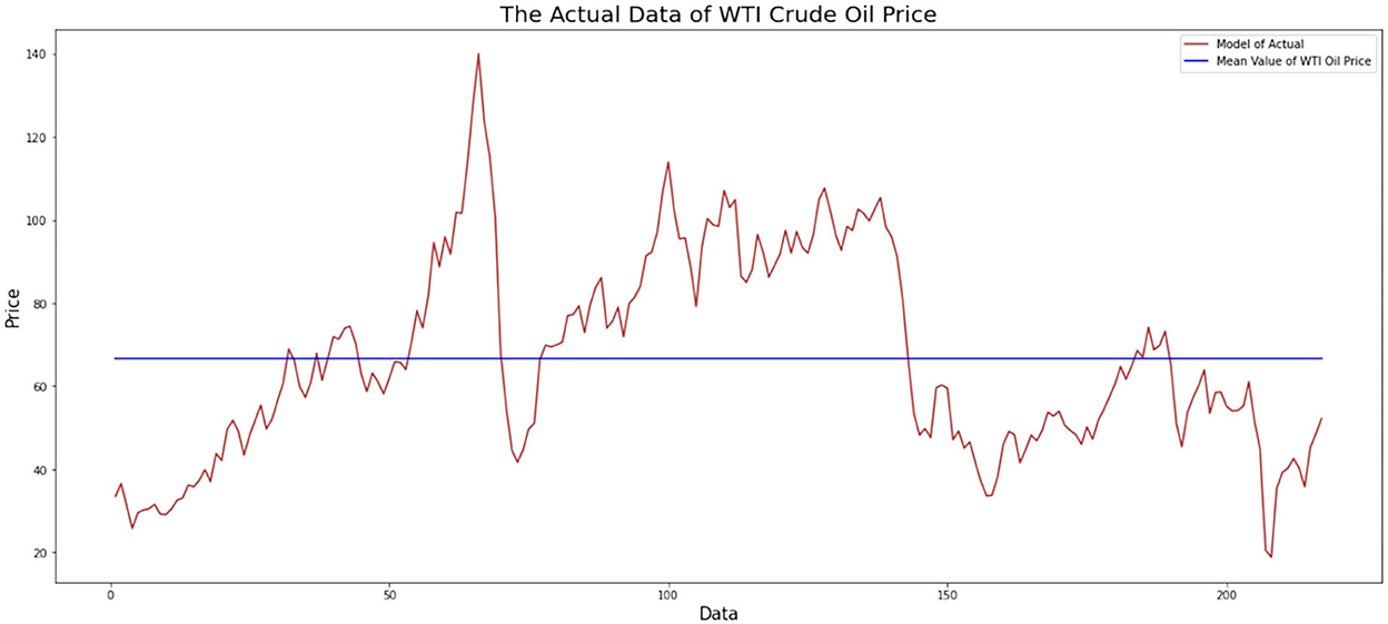
Figure 1. WTI oil price monthly data plot.

Figure 1 indicates that the monthly data on WTI oil prices has an uptrend and a downtrend at certain times. The data do not fluctuate around the mean, and the variance is not constant during observation. The data can be stationary to the variance and mean by performing a Box–Cox transformation and differentiating the data, respectively. The result of parameter Box–Cox, that is 0.3839, means that the data will be transformed as exponential with that parameter once to get the new data. At the same time, the uptrend and a downtrend fluctuation at certain times indicated that the ADF test is required. The result of the ADF test is shown in Table 1.

TABLE 1

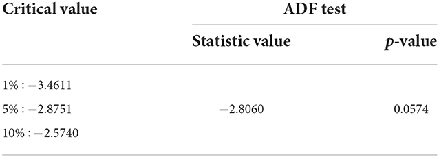
Table 1. Augmented Dickey–Fuller test.

It indicates that the mean of the data is not stationary yet. Furthermore, the exchange rate data have to make a difference. The plot of the transformed data on WTI oil prices is shown in Figure 2.

FIGURE 2

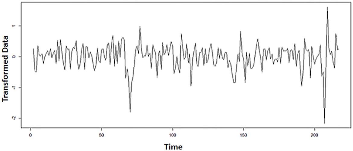
Figure 2. WTI oil data plot after transformation and differencing.

Based on Figure 2, it shows that the data have spread around the mean and variance. In other words, the data are stationary concerning the mean and variance. Next, identify the order of the ARIMA model by looking at the ACF and PACF plots as follows:

From Figure 3, it shows that the significant values of the ACF and PACF coefficients are the same at lag 1, so the ARIMA(p,d,q) model can be chosen with the order p and q equal to 1. And because differencing is carried out once, the order differencing is equal to 1. Thus, the possible models are ARIMA(1,1,0), ARIMA(1,1,1), and ARIMA(0,1,1). Next, the results of the estimation of the parameters for each model are shown in Table 2.

FIGURE 3

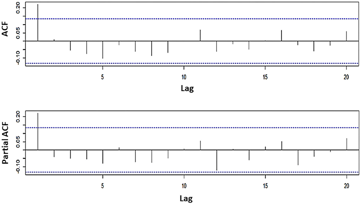
Figure 3. ACF and PACF plots of WTI oil data.

TABLE 2

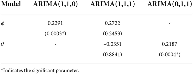
Table 2. Parameter estimation ARIMA(p,d,q) model with its probability value.

Then the parameter significance test is carried out by determining the probability value of the model parameters. The model is indicated to be significant if the probability value of the model is smaller than 0.05, which means that the ARIMA(1,1,0) and ARIMA(0,1,1) models are significant and ready to be applied. After testing the significance of the parameters, the next step is to choose the best model from the significant model by comparing the AIC and BIC values for each model which is presented in Table 3.

TABLE 3

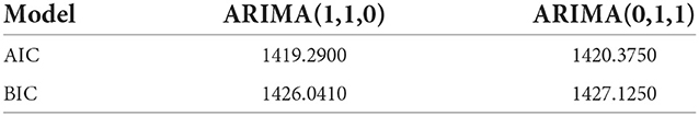
Table 3. Comparison of AIC and BIC values ARIMA(p,d,q) model.

From the comparison of AIC and BIC values in Table 3 for the three models, it can be observed that the ARIMA(1,1,0) model has the smallest AIC and BIC values among other models. So it can be concluded that the best model is the ARIMA(1,1,0) model. The residual assumption test of the ARIMA (1,1,0) model is shown in Table 4.

TABLE 4

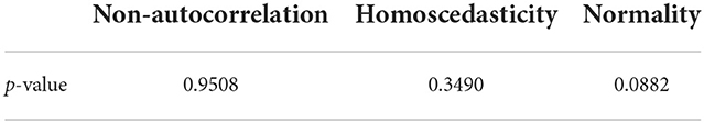
Table 4. Residual assumption test ARIMA(1,1,0) model.

Based on Table 4, it shows that the p-value of the non-autocorrelation and homoscedasticity test is p-value greater than 0.05. It means that there is no correlation between the data residuals, and the variance of the residuals is the same every time (homoscedasticity). Meanwhile, in the normality test, the p-value which is greater than 0.05 identifies that the residual data are normally distributed. So, the ARIMA(1,1,0) model is obtained as the best model that fulfills the residual assumptions.

3.2. The ARFIMA model of WTI oil price

The first step is to check that WTI oil data are stationary against variance. Next, consider the ACF plot of the stationary WTI oil data against the variance to see the long-memory pattern as shown in Figure 4.

FIGURE 4

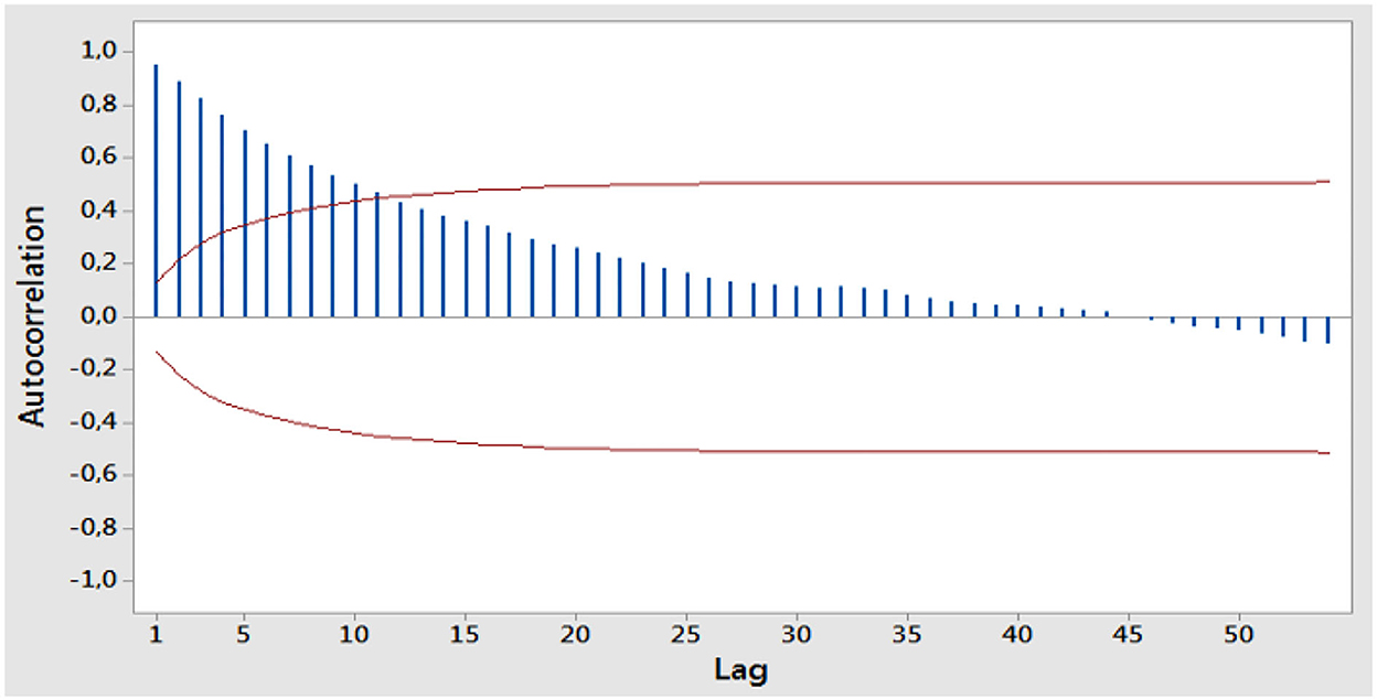
Figure 4. ACF plot of stationary WTI oil data against variance.

Based on Figure 4, it shows that the data decrease slowly over time, which means that the data have a long-memory pattern. Furthermore, the estimation of differencing parameters is determined by using the GPH method in order to obtain the d_GPH value of d. Then, differencing the stationary data on the variance with a value of d_GPH has been obtained. Furthermore, the ARFIMA model was identified by looking at the ACF and PACF plots as follows:

Figure 5 indicates that the significant ACF coefficient value reaches lag 5, while the significant PACF coefficient value is at lag 1. Thus, there are 11 possible ARFIMA models. The next step is to estimate the parameter and its probability value for each model, whose results are shown in Table 5.

FIGURE 5

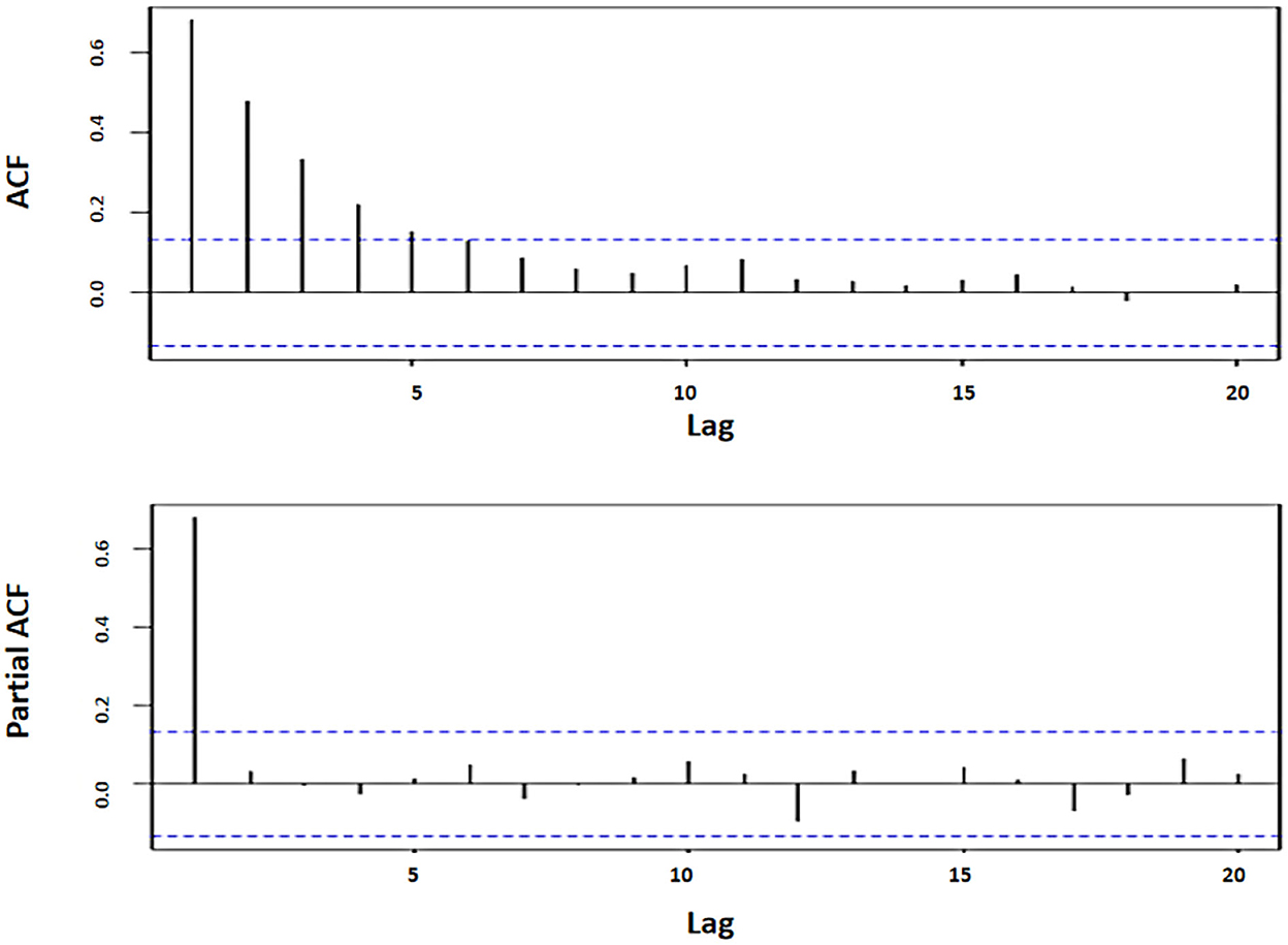
Figure 5. ACF and PACF plots of WTI oil data.

TABLE 5

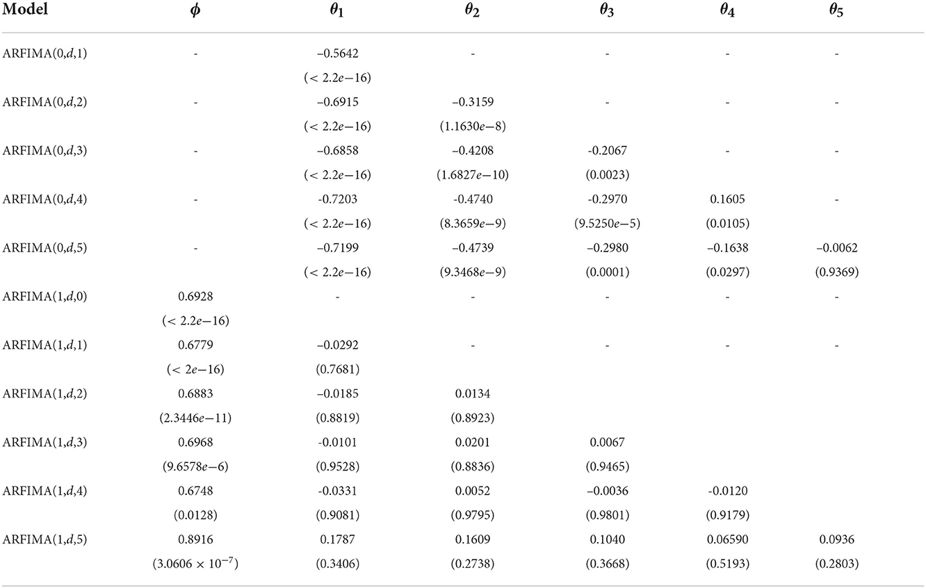
Table 5. Parameter estimation ARFIMA(p,d,q) model with d = 0.4943.

Based on Table 5, the significant models have a smaller probability value than the significant level. There are ARFIMA(0, d, 1), ARFIMA(0, d, 2), ARFIMA(0, d, 3), ARFIMA(0, d, 4), and ARFIMA(1, d, 0) which are included as significant models and already used for forecasting new data. The next step is to choose the best model by comparing the AIC and BIC values for each model presented in Table 6.

TABLE 6

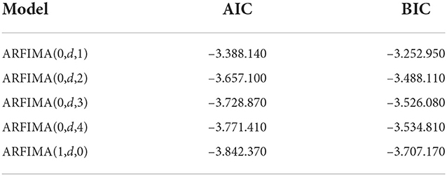
Table 6. Comparison of AIC and BIC values ARFIMA (p,d,q) model with d = 0.4943.

From the comparison of AIC and BIC values in Table 7 for the five models, it can be observed that the ARFIMA(1,d.0) model has the smallest AIC and BIC values among other models. So it can be concluded that the best model is the ARFIMA(1,d,0) model. The following residual assumption test of the ARFIMA model (1,d.0) is shown in Table 8.

TABLE 7

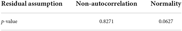
Table 7. Residual assumption test ARFIMA(1,d,0) model with d = 0.4943.

TABLE 8

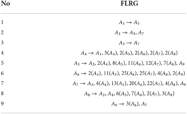
Table 8. The fuzzy logic relation group (FLRG).

Based on Table 8, it describes that the non-autocorrelation test has a p-value greater than 0.05. It means that there is no correlation between the data residuals. Moreover, the normality test obtained a p-value greater than 0.05, which shows that the residuals are normally distributed. So the ARFIMA(1,d.0) model is obtained as the best model that fulfills the residual assumption.

3.3. The hybrid ARIMA-FTSMC model of WTI oil price

The hybrid ARIMA-FTSMC model is a combination of the ARIMA and FTSMC models. The first step is to build a model of time series data with the ARIMA model. The results show that the ARIMA(1,1,0) model is selected to be the best model. Thus, the residual data of the ARIMA(1,1,0) model, denoted by ε_t, are built using the FTSMC model. In the form of a negative number, the transformation is carried out so that the data become a non-negative number. The data transformation is used to determine the minimum data from the residual data. Then, the residual data are subtracted from the minimum data to become a non-negative number. Based on the residual data, the result shows the minimum residual data is d_min = −29.2866. Suppose the residual data at the time t = 3, which is ε₃ = −6.2987 so that the residual transformation data obtained is 22.9878. The first step in the modeling residual data using the FTSMC model is to determine the union of set U. Based on the residual transformation data, it is obtained that D_max = 46.3287 and D_min = 0. Then, the values are set as D₁ = 0 and D₂ = 0.6713 that is associated with D_min and D_max so that the lower and upper bound in the interval will always include the data to ignore the outlier data. The union of set U is defined as an interval below:

$\begin{array}{l}U=[D_{min}-D_1,D_{max}+D_2)=[0-0,46.3287+0.6713)\\ =[0,47).& (26)\end{array}$

The union of sets U is divided into n intervals with the same interval length using the Sturges formula so that the value is obtained n = 9 and interval length of l = 5.2222. The obtained intervals are u₁ = [0.0000, 5.2222), u₂ = [5.2222, 10.4444), u₃ = [10.4444, 15.6667), u₄ = [15.6667, 20.8889), u₅ = [20.8889, 26.1111), u₆ = [26.1111, 31.3333), u₇ = [31.3333, 36.5556), u₈ = [36.5556, 41.7778), and u₉ = [41.7778, 47.0000). The next step is transforming the residual data into linguistic values, which are also in the form of intervals. Suppose the residual transformation data at the time t = 1 is 29.3201. It goes into the interval u₆. As a result, the transformation data at t = 1 after fuzzyfication are A₆.

Then, in the fuzzy logic relation (FLR) step, there is a relationship between the order of the data to the transformed data. This relationship is expressed by A_i→A_j, where A_i is the left-hand side (LHS), and A_j is the right-hand side (RHS) from FLR. For example, FLR on a fuzzy set with value A₄ has a displacement relationship to A₄ or A₄→A₄. Therefore, the appearance of FLR A₄→A₄ is 3 on the data obtained so that fuzzy logic relation group (FLRG) from A₄ to A₄ can be written as A₄ → 3(A₄). FLRG for all data is shown in Table 8.

The fuzzy set relation above shows that FLR is in one group. The purpose of the relation states that the fuzzy set on the left side only has a relationship with the fuzzy set on the right side. For example, by using FLRG in Table 8, the transition probability matrix R, which has order 9, can be obtained as follows:

$\begin{array}{ll}\text{R}=\left[\begin{array}{ccccccccc}0& 0& 0& 0& 1& 0& 0& 0& 0\\ 0& 0& 0& 0& \frac{1}{2}& 0& \frac{1}{2}& 0& 0\\ 0& 0& 0& 0& 0& 0& 1& 0& 0\\ \frac{1}{12}& 0& 0& \frac{3}{12}& \frac{2}{12}& \frac{2}{12}& \frac{2}{12}& \frac{1}{12}& 0\\ 0& \frac{1}{42}& 0& \frac{2}{42}& \frac{8}{42}& \frac{11}{42}& \frac{12}{42}& \frac{7}{42}& \frac{1}{42}\\ 0& 0& 0& \frac{2}{69}& \frac{11}{69}& \frac{25}{69}& \frac{25}{69}& \frac{4}{69}& \frac{2}{69}\\ 0& 0& \frac{1}{65}& \frac{4}{65}& \frac{13}{65}& \frac{20}{65}& \frac{22}{65}& \frac{4}{65}& \frac{1}{65}\\ 0& \frac{1}{20}& 0& \frac{1}{20}& \frac{6}{20}& \frac{7}{20}& \frac{2}{20}& \frac{3}{20}& 0\\ 0& 0& 0& 0& 0& \frac{3}{4}& \frac{1}{4}& 0& 0\end{array}\right].& (27)\end{array}$

The next step is to calculate the initial modeling value using the R matrix above. Using Equation 15, the initial modeling values for the residual transformation data at t = 2 are as follows:

$\begin{array}{l}{F}_2=m_4{P}_{64}+m_5{P}_{65}+X_1{P}_{66}+m_7{P}_{67}+m_8{P}_{68}+m_9{P}_{69}\\ =(18.2778)\left(\frac{2}{69}\right)+(23.5000)\left(\frac{11}{69}\right)+(29.3201)\left(\frac{25}{69}\right)\\ +(33.9444)\left(\frac{25}{69}\right)+(39.1667)\left(\frac{4}{69}\right)+(44.3889)\left(\frac{2}{69}\right)\\ =\mathrm{30.7553.}\end{array}$

Then the modeling adjustment value for the residual transformation data at t = 2 is

$\begin{array}{l}{D}_t=\left(\frac{l}{2}\right)s=\left(\frac{5.2222}{2}\right)\left(1\right)=2.6111.\end{array}$

Final modeling values for residual transformation data at time t = 2 are:

$\begin{array}{lll}F{M}_2& =& F_2+D_t=30.7553+2.6111=33.3664.\end{array}$

Transformation returns to return the final modeling residual transformation data to the initial modeling residual data. This is done by adding the minimum residual data to the final modeling residual transformation data. For example when t = 2, the final modeling value of residual data with FTSMC is 33.3664+(−−29.2866) = 4.0798. The results of the ARIMA-FTSMC hybrid modeling were obtained by adding the ARIMA(1,1,0) model data with the final ARIMA(1,1,0) residual modeling data. For example, when t = 2, the hybrid modeling value is 33.5996+4.0798 = 37.6794.

3.4. The hybrid ARFIMA-FTSMC model of WTI oil price

The hybrid ARFIMA-FTSMC model is a combination of the ARFIMA and FTSMC models. The first step is to build a model of time series data with the ARFIMA model. The results show that the ARFIMA(1,d,0) model is selected to be the best model. Thus, the residual data of the ARFIMA(1,d,0) model, denoted by ϵ_t, is built using the FTSMC model. In the form of a negative number, the transformation is carried out so that the data becomes a non-negative number. The data transformation is used to determine the minimum data from the residual data. Then, residual data are subtracted from the minimum data to become a non-negative number. Based on the residual data, the result shows the minimum residual data is d_min = −26.8005. suppose the residual data at the time t=3, which is ϵ₃ = −6.2003 so that the residual transformation data obtained is 20.6002. The first step in modeling residual data using the FTSMC model is to determine the union of set U. Based on the residual transformation data. It is obtained that D_max = 43.6958, D_min = 0 and the determination of value D₁ = 0, D₂ = 1.3042. The union of set U is defined as an interval below:

$\begin{array}{l}U=[D_{min}-D_1;D_{max}+D_2)=[0-0;43.6958+1.3042)\\ =[0;45)\end{array}$

The union of sets U is divided into n intervals with the same interval length using the Sturges formula so that the value is obtained n=9 and interval length of l = 5. The obtained intervals are u₁ = [0, 5), u₂ = [5, 10), u₃ = [10, 15), u₄ = [15, 20), u₅ = [20, 25), u₆ = [25, 30), u₇ = [30, 35), u₈ = [35, 40), u₉ = [40, 45). The next step is transforming the residual data into linguistic values, which are also in the form of intervals. Suppose the residual transformation data at the time t = 2 is 29.7330 it goes to interval u₆. As a result, the transformation data at time t = 2 after fuzzyfication is A₆.

Then, in the fuzzy logic relation (FLR) step, there is a relationship between the order of the data to the transformed data. This relationship is expressed by A_i→A_j, where A_i is the left-hand side (LHS), and A_j is the right-hand side (RHS) from FLR. For example, FLR on a fuzzy set with value A₄ has a displacement relationship to A₄ or A₄→A₄. Therefore, the appearance of FLR A₄→A₄ is 3 on the data obtained so that the fuzzy logic relation group (FLRG) from A₄ to A₄ can be written as A₄ → 3(A₄). FLRG for all data is shown in Table 9:

TABLE 9

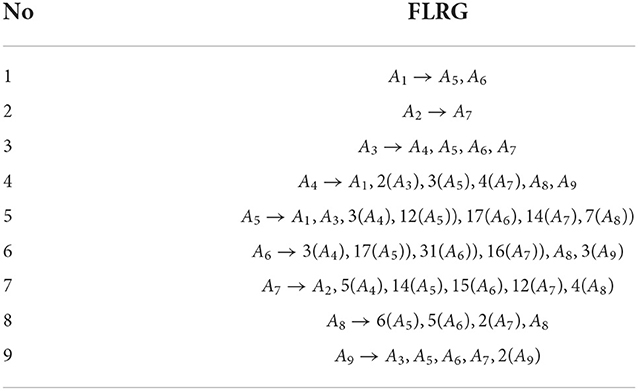
Table 9. The fuzzy logic relation group (FLRG).

The fuzzy set relation above shows that FLR is in one group. The purpose of the relation states that the fuzzy set on the left side only has a relationship with the fuzzy set on the right side. For example, by using FLRG in Table 8, the transition probability matrix R, which has order 9, can be obtained as follows:

$\begin{array}{ll}\text{R}=\left[\begin{array}{ccccccccc}0& 0& 0& 0& \frac{1}{2}& \frac{1}{2}& 0& 0& 0\\ 0& 0& 0& 0& 0& 0& 1& 0& 0\\ 0& 0& 0& \frac{1}{4}& \frac{1}{4}& \frac{1}{4}& \frac{1}{4}& 0& 0\\ \frac{1}{12}& 0& \frac{2}{12}& 0& \frac{3}{12}& 0& \frac{4}{12}& \frac{1}{12}& \frac{1}{12}\\ \frac{1}{55}& 0& \frac{1}{55}& \frac{3}{55}& \frac{12}{55}& \frac{17}{55}& \frac{14}{55}& \frac{7}{55}& 0\\ 0& 0& 0& \frac{3}{71}& \frac{17}{71}& \frac{31}{71}& \frac{16}{71}& \frac{1}{71}& \frac{3}{71}\\ 0& \frac{1}{51}& 0& \frac{5}{51}& \frac{14}{51}& \frac{15}{51}& \frac{12}{51}& \frac{4}{51}& 0\\ 0& 0& 0& 0& \frac{6}{14}& \frac{5}{14}& \frac{2}{14}& \frac{1}{14}& 0\\ 0& 0& \frac{1}{6}& 0& \frac{1}{6}& \frac{1}{6}& \frac{1}{6}& 0& \frac{2}{6}\end{array}\right].& (28)\end{array}$

The next step is to calculate the initial modeling value using the R matrix above. The initial modeling values for the residual transformation data at t = 4 are as follows:

$\begin{array}{l}{F}_4=m_1{P}_{51}+m_3{P}_{53}+m_4{P}_{54}+X_3{P}_{55}+m_6{P}_{56}+m_7{P}_{57}+m_8{P}_{58}\\ =(2.5)\frac{1}{55}+(12.5)\frac{1}{55}+(17.5)\frac{3}{55}+(20.6002)\frac{12}{55}+(27.5)\frac{17}{55}\\ +(32.5)\frac{14}{55}+(37.5)\frac{7}{55}\\ =\mathrm{27.2673.}\end{array}$

Then the modeling adjustment value for the residual transformation data at t = 2 is

$\begin{array}{lll}{D}_t& =& \left(\frac{l}{2}\right)s=\left(\frac{5}{2}\right)\left(0\right)=0.\end{array}$

Final modeling values for residual transformation data at time t = 2 are:

$\begin{array}{lll}F{M}_4& =& F_4+D_t=27.2673+0=27.2673.\end{array}$

Transformation return to return the final modeling residual transformation data to the initial modeling residual data. This is done by adding the minimum residual data to the final modeling residual transformation data. For example when t=4, the final modeling value of residual data with FTSMC is 27.2673+(-26.8005)=0.4668. The results of the ARFIMA-FTSMC hybrid modeling were obtained by adding the ARFIMA(1,d,0) model data with the final ARFIMA(1,d,0) residual data. For example, when t=4, the hybrid modeling value is 29.8487+0.4668=30.3156.

3.5. The comparison and discussion

After building the model of ARIMA, ARFIMA, a hybrid model of ARIMA-FTSMC, and a hybrid model of ARFIMA-FTSMC, then, we continue to do comparisons among the models by analyzing graphical and accuracy measurements. The following is a graphical comparison of the ARIMA, ARFIMA, hybrid ARIMA-FTSMC, and hybrid ARFIMA-FTSMC models based on the WTI data presented in Figure 6 below:

FIGURE 6

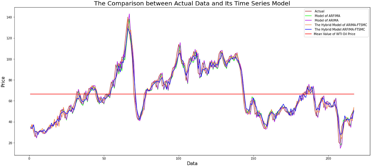
Figure 6. Comparison graph of actual data with ARIMA, ARFIMA, hybrid ARIMA-FTSMC, and hybrid ARFIMA-FTSMC models.

From Figure 6, it can be seen that modeling using ARIMA, ARFIMA, hybrid ARIMA-FTSMC, and hybrid ARFIMA-FTSMC models provide modeling results that are close to the actual data. Although graphically, the three models show good estimation results, it is necessary to examine the level of accuracy of each model to see a more precise model with better accuracy that can be used in predictions.

Calculation of modeling accuracy to see the preferred model for modeling WTI oil price data from the three models is presented using MAE, RMSE, and MAPE values. By using Equations (22)–(24), the modeling accuracy is shown in Table 10.

TABLE 10

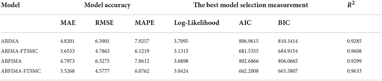
Table 10. The comparison of the ARIMA model with GARCH, FFNN, and GARCH-FFNN using model accuracy, the best model selection, and goodness of fit R².

Table 10 shows the accuracy measures, the best selection criteria, and the goodness of fit for each model. Based on the MAE and RMSE values, all models have accuracy values that are not too far off. When viewed from the MAPE criteria, all models have a MAPE value of less than 10%. This means that all models can model WTI oil data very well. Based on the accuracy of the model, the ARFIMA-FTSMC has the best performance than the rest model, and so does the best selection and the goodness of fit criterion. Table 10 shows that the ARFIMA-FTSMC has the smallest value of MAE, RMSE, MAPE, Log-likelihood, AIC, and BIC. Then, the second one is ARIMA-FTSMC which has the model accuracy and goodness of fit that is closer to ARFIMA-FTSMC. It shows that if the FTSMC model adjusts the residual model of ARIMA or ARFIMA then the accuracy and goodness of fit of the new proposed model will be better than the model without improvements using FTSMC. Therefore, the hybrid model of ARFIMA-FTSMC gives better results in modeling monthly WTI oil prices than the rest models.

4. Conclusion

Based on the data analysis that has been done, it can be seen that the WTI oil data have a long-memory data pattern. This value is detected from the ACF plot, which decreases slowly over time. This shows the influence of past data on the current data is still strong and will decrease over time. Therefore, time series data for WTI oil prices can be formed into the model of ARIMA, the model of ARFIMA, the hybrid model of ARIMA-FTSMC, and the hybrid model of ARFIMA-FTSMC. The four models provide reasonable parameter estimates and high accuracy, which shows their closeness to the actual data. This is obtained based on the accuracy value of each model obtained not too far from the actual data. However, the proposed new model, the hybrid model of ARFIMA-FTSMC, provides the smallest MAE, RMSE, and MAPE values. It can be concluded that the hybrid model of ARFIMA-FTSMC has better accuracy than other models.

Data availability statement

Publicly available datasets were analyzed in this study. This data can be found at: https://www.eia.gov/.

Author contributions

DD contributed to the conception of the hybrid model and design of the study. KR played a role in analyzing the model of the fuzzy time series (FTS) and wrote sections of the article. M and YA performed the time series analysis of ARIMA and ARFIMA, respectively. MY organized the database and numerical simulation of data processing. All authors contributed to the article revision, read, and approved the submitted version.

Acknowledgments

The authors acknowledge Andalas University under the Ministry of Education, Cultural, Research and Technology for funding this research under the scheme of university basic research excellency with contract number 011/E5/PG.02.00.PT.2022.

Conflict of interest

The authors declare that the research was conducted in the absence of any commercial or financial relationships that could be construed as a potential conflict of interest.

Publisher's note

All claims expressed in this article are solely those of the authors and do not necessarily represent those of their affiliated organizations, or those of the publisher, the editors and the reviewers. Any product that may be evaluated in this article, or claim that may be made by its manufacturer, is not guaranteed or endorsed by the publisher.

References

1. Wei WWS. Multivariate Time Series Analysis and Applications. New York, NY: Wiley (2019).

Google Scholar

2. Ramadani K, Devianto D. The forecasting model of Bitcoin price with fuzzy time series Markov chain and chen logical method. AIP Conf Proc. (2020) 2296:1–11. doi: 10.1063/5.0032178

CrossRef Full Text | Google Scholar

3. Devianto D, Maiyastri, Fadhilla DR. Time series modeling for risk of stock price with value at risk computation. Appl Math Sci. (2015) 9:2779–87. doi: 10.12988/ams.2015.52144

CrossRef Full Text | Google Scholar

4. Mohammad AA, Mudhir AA. Dynamical approach in studying stability condition of exponential (GARCH) models. J King Saud Univer Sci. (2020) 32:272–8. doi: 10.1016/j.jksus.2018.04.028

CrossRef Full Text | Google Scholar

5. Zeghdoudi H, Amrani M. On mixture GARCH models: long, short memory and application in finance. J Math Stat Stud. (2021) 2:01–07. doi: 10.32996/jmss.2021.2.2.1

CrossRef Full Text | Google Scholar

6. Park SH, Griffiths JD, Longtin A, Lefebvre J. Persistent entrainment in non-linear neural networks with memory. Front Appl Math Stat. (2018) 4:31. doi: 10.3389/fams.2018.00031

CrossRef Full Text | Google Scholar

7. Garnier J, K Solna K. Implied volatility structure in turbulent and long-memory markets. Front Appl Math Stat. (2020) 6:10. doi: 10.3389/fams.2020.00010

CrossRef Full Text | Google Scholar

8. Baillie RT, Morana C. Adaptive ARFIMA models with applications to inflation. Econ Model. (2012) 29:2451–9. doi: 10.1016/j.econmod.2012.07.011

CrossRef Full Text | Google Scholar

9. Baillie RT, Kongcharoen C, Kapetanios G. Prediction from ARFIMA models: comparisons between MLE and semiparametric estimation procedures. Int J Forecast. (2012) 28:46–53. doi: 10.1016/j.ijforecast.2011.02.012

CrossRef Full Text | Google Scholar

10. Zhang X, Lu Z, Wang Y, Zhang R. Adjusted jackknife empirical likelihood for stationary ARMA and ARFIMA models. Stat Probab Lett. (2020) 165:1–11. doi: 10.1016/j.spl.2020.108830

CrossRef Full Text | Google Scholar

11. Boaisha SM, Amaitik SM. Forecasting model based on fuzzy time series approach. In: Proceedings of the 10th International Arab Conference on Information Technology-ACIT. (2010). p. 14–16.

Google Scholar

12. Efendi R, Deris MM. Forecasting of malaysian oil production and oil consumption using fuzzy time series. Recent Adv Soft Comput Data Min. (2016) 441:31–40. doi: 10.1007/978-3-319-51281-5_4

CrossRef Full Text | Google Scholar

13. Tsaur RC. A fuzzy time series-markov chain model with an application to model the exchange rate between the taiwan and US dollar. Int J Innovat Comput Inf Control. (2012) 8:4931–42.

Google Scholar

14. Uzun B, Kıral E. Application of Markov chains-fuzzy states to gold price. Procedia Comput Sci. (2017) 120:365–71. doi: 10.1016/j.procs.2017.11.251

CrossRef Full Text | Google Scholar

15. Gao R, Duru O. Parsimonious fuzzy time series modelling. Expert Syst Appl. (2020) 156:1–12. doi: 10.1016/j.eswa.2020.113447

CrossRef Full Text | Google Scholar

16. Yollanda M, Devianto D, Yozza H. Nonlinear modeling of IHSG with artificial intelligence. In: 2018 International Conference on Applied Information Technology and Innovation. Padang: IEEE Xplore (2018). p. 85–90.

Google Scholar

17. Adib A, Zaerpour A, Lotfirad M. On the reliability of a novel MODWT-based hybrid ARIMA-artificial intelligence approach to forecast daily snow depth (Case study: the western part of the Rocky Mountains in the USA). Cold Regions Sci Technol. (2021) 189:1–11. doi: 10.1016/j.coldregions.2021.103342

CrossRef Full Text | Google Scholar

18. Denis DJ. Applied Univariate, Bivariate, and Multivariate Statistics: Understanding Statistics for Social and Natural Scientists, with Applications in SPSS and R. New York, NY: Wiley (2021).

Google Scholar