Numerical analysis of finite difference schemes arising from time-memory partial integro-differential equations

1. Introduction

The realm of differential equations is full of various categories of differential equations. When the differential equation has one independent variable is called an ordinary differential equation (ODE). In comparison, it has more than one called a partial differential equation (PDE). An equation contains an unknown function in the integral operator, known as an integral equation (IE). An integro-differential equation (IDE) is an equation that includes the derivatives and integration of the unknown function with one independent variable. For an unknown function with several independent variables, it is called a partial integro-differential equation (PIDE). Besides that, there is a classification based on the linearity of the unknown function. Partial differential equations (PDEs) are used to model several complicated phenomena in physics, chemistry, biology, and finance. They exhibit versatility in various models. However, there are so many phenomena in these fields that PDEs fail to model them. Because they need to consider their hierarchical status, we can split them into two main categories; the first requires considering its status in past time, and the second demand considering the accumulation behavior for one of its variables (spatial variable). The first category is represented by a convolution on the time variable by Yanik and Fairweather [1], while the second uses the convolution in the spatial variable [2].

Moreover, some phenomena use nonlocal operators in non-convolution forms, such as options under the Lévy process and Bates models [3–5]. Here comes the importance of integro-differential equations (IDEs) and partial integro-differential equations (PIDEs), which use the nonlocal operator to capture the behaviors of these phenomena. There are enormous physical, economic, and biological phenomena modeled based on these equations. For instance, neural IDEs are used to model brain dynamics, and it has been investigated based on the deep learning framework, see Zappala et al. [6]. The population dynamics are modeled based on nonlinear PIDEs and solved using the pseudo-spectral technique [2]. Various categories of IDEs are studied using different numerical techniques, see Mirzaee and Rafei [7], Mirzaee and Piroozfar [8], and Sakran [9].

Many researchers solved PIDEs using different mathematical techniques, which can be classified into two main categories: numerical [10–12] and spectral techniques [2, 13, 14]. The collocation method has been adapted to solve a broad class of PIDEs, see Yüzbaşı and Yıldırım [15] and Xu [11]. The Pell-Lucas collocation method is used to solve the parabolic PIDEs [15]. A space-time Sinc collocation technique is applied to obtain numerical solutions of a PIDE with a weak-singular integral-kernel [11]. In Kumar and Vijesh [16], the authors solved a two-spatial dimension PIDE of the memory type based on the Legendre wavelet iterative method. Also, the numerical methods are extended to solve fractional PIDEs [14, 17]. For instance, Caputo-Fabrizio fractional Volterra PIDEs are solved using Legendre-Gauss-Lobatto quadrature incorporated with shifted Hahn polynomials, see Dehestani and Ordokhani [14]. Here, we consider a one spatial dimension parabolic partial differential equation with a source term and incorporated with a nonlocal integral part, given by

$\begin{array}{ll}{\partial }_{\tau }{V}={\partial }_x^2{V}+F(x,\tau )-{\displaystyle {\int }_0^{\tau }}{K}(x,\tau -s){V}(x,s)ds,x\in \Omega ,\tau >0,& (1)\end{array}$

subjected to initial and boundary conditions

$\begin{array}{ll}{V}(x,0)=g(x),x\in \Omega ,{V}(x,\tau )={\varphi }_x(\tau ),x\in \Gamma ,\tau >0,& (2)\end{array}$

where, F(x, τ) represents the source function, ${K}(x,\tau -s)$ is the kernel of integration, and Ω ∪ Γ = [0, L]. The problem (Equations 1, 2) is used to describe the behavior of a continuous medium nuclear reactor such that the unknown function represents the total reactor power and also a wide class of models in thermoelasticity, viscoelasticity, refer to Lakshmikantham [18, Chap. 5]. Most mathematical techniques that are used to solve the problem (Equations 1, 2) treat the discretization of the unknowns in an integral part by applying additional expansion to make them coincide with the unknowns of the differential part consequently, increasing the computational time cost. Here, we introduce a mathematical treatment to overcome this issue.

The outline of the paper is as follows. Section 2 is dedicated to constructing the corresponding finite difference scheme of the problem (Equations 1, 2). The differential part is discretized using θ-finite difference approximations, while the integral part is discretized using Simpson's rule incorporated with the Heaviside step function. It is used to convert the variable upper bound of an integral part into a constant without adding any numerical computational cost, which is discussed in detail next section. To the best of our knowledge, we are the first authors who introduced this idea. The stability analysis of the proposed scheme is studied based on the second norm of matrices and Gerschgoren's theorems in Section 3. The consistency is discussed in Section 4. In Section 5, several examples are implemented to reveal the versatility and reliability of the proposed technique.

2. The finite difference scheme establishment

We start this section with the construction of the numerical grid of the computational domain (x, τ) ∈ [0, L] × [0, T], where T is the total elapsed time, the time variable τ is discretized using uniform mesh-points τ_n = nΔτ, Δτ = T/N_τ, and the spatial variable x is divided into subintervals of equal length using the spatial nodes x_k = kΔx, Δx = L/N_x, N_τ, and N_x is the total number of subintervals. Let $V_k^n$ be the approximation of ${V}$ at the point (x_k, τ_n). The first-time partial derivative is approximated by

$\begin{array}{ll}{\partial }_{\tau }{V}\approx \frac{V_k^{n+1}-V_k^n}{\Delta \tau },& (3)\end{array}$

and the second spatial derivative is discretized based on the θ-method, which incorporates a combination of explicit-implicit discretization, given by

$\begin{array}{l}{\partial }_x^2{V}\approx \frac{\theta }{{(\Delta x)}^2}\left(V_{k+1}^{n+1}-2V_k^{n+1}+V_{k-1}^{n+1}\right)+\frac{(1-\theta )}{{(\Delta x)}^2}\\ \hfill \left(V_{k+1}^n-2V_k^n+V_{k-1}^n\right).& (4)\end{array}$

The θ-parameter is responsible for the ratio between explicit and implicit finite difference schemes, and its value θ ∈ [0, 1]. When θ = 0, then we have an explicit scheme, while it is a fully implicit scheme for θ = 1. For θ ∈ (0, 1), it represents a combination of explicit and implicit schemes. From Equations (3) and (4) into Equation (1), we have

$\begin{array}{ll}A\left[V_k^{n+1}\right]=B\left[V_k^n\right]+\Delta \tau F_k^n-\Delta \tau {\displaystyle {\int }_0^{{\tau }_n}}{{K}}_k({\tau }_n-s)V_k(s)ds,& (5)\end{array}$

$k=1,2,\dots ,N_x-1,\text{and }n=0,1,\dots ,N_{\tau }-1,$

where, A and B are difference operators, given by

$\begin{array}{l}A\left[V_k^{n+1}\right]=(1+2\theta r)V_k^{n+1}-\theta r(V_{k+1}^{n+1}+V_{k-1}^{n+1}),\\ B\left[V_k^n\right]=(1-2\tilde{\theta }r)V_k^n+\tilde{\theta }r(V_{k+1}^n+V_{k-1}^n),\\ r=\frac{\Delta \tau }{{(\Delta x)}^2},\tilde{\theta }=1-\theta .\end{array}$

To obtain the first time-level, we put n = 0 into Equation (5), then the lower and upper bounds become equal; consequently, the integral part vanishes, and the first time-level becomes

$\begin{array}{ll}A\left[V_k^1\right]=B\left[V_k^0\right]+\Delta \tau F_k^0.& (6)\end{array}$

The integral part of Equation (5) has two drawbacks; the first one is the upper bound of the integration changing as the index n changes, so, for each time level, we have a different integral interval. The second drawback appears when we try to apply a suitable substitution that converts the interval of variable length into an interval with a fixed size. It leads to the discretization of V_k(s) does not coincide with the unknowns $V_k^n$ at the constructing mesh points; in other words, it gives new unknowns other than $V_k^n$. To overcome the first drawback, we use the Heaviside step function ${H}(\tau -a)$, which is defined by

${H}(\tau -a)=\{\begin{array}{ll}0,& \hfill 0\le \tau <a,\\ 1,& \hfill \tau \ge a,\end{array}$

consequently, the integral part of Equation (5) is rewritten as

$\begin{array}{l}{{I}}_k({\tau }_n)={\displaystyle {\int }_0^{{\tau }_n}}{{K}}_k({\tau }_n-s)V_k(s)ds\\ ={\displaystyle {\int }_0^1}{{K}}_k({\tau }_n-s)V_k(s)\left(1-{H}(s-{\tau }_n)\right)ds.& (7)\end{array}$

Next, we approximate the integration based on Simpson's rule

$\begin{array}{c}{{I}}_k({\tau }_n)\approx I_k^n=\frac{\Delta s}{3}({{K}}_k({\tau }_n-s_0)V_k^0\\ +4{\displaystyle \sum _{j=1}^{N_{\tau }/2}}{{K}}_k({\tau }_n-s_{2j-1})V_k^{2j-1}\left(1-{H}(s_{2j-1}-{\tau }_n)\right)+\\ 2{\displaystyle \sum _{j=1}^{N_{\tau }/2-1}}{{K}}_k({\tau }_n-s_{2j})V_k^{2j}(1-{H}(s_{2j}-{\tau }_n))).& (8)\end{array}$

Here, we discretize the interval of integration as the same as the discretization of the time variable, i.e., Δs = Δτ, and s_j = τ_j, j = 0, 1, …, N_τ to guarantee the resultant unknowns $V_k^j$ coincide with the original unknowns $V_k^n$, consequently, Equation (8) becomes

$\begin{array}{c}{I}_k^n=\frac{\Delta \tau }{3}({{K}}_k({\tau }_n-{\tau }_0)V_k^0+4{\displaystyle \sum _{j=1}^{N_{\tau }/2}}{{K}}_k({\tau }_n-{\tau }_{2j-1})\\ V_k^{2j-1}(1-{H}({\tau }_{2j-1}-{\tau }_n))+\\ 2{\displaystyle \sum _{j=1}^{N_{\tau }/2-1}}{{K}}_k({\tau }_n-{\tau }_{2j})V_k^{2j}(1-{H}({\tau }_{2j}-{\tau }_n))).& (9)\end{array}$

The discretization of initial and boundary conditions is given by

$V_k^0=g_k,V_0^n={\varphi }_0^n,V_{N_x}^n={\varphi }_{N_x}^n.$

Hence, the finite difference problem becomes

$\begin{array}{ll}\begin{array}{l}A\left[V_k^1\right]=B\left[V_k^0\right]+\Delta \tau F_k^0,\\ A\left[V_k^{n+1}\right]=B\left[V_k^n\right]+\Delta \tau F_k^n-\Delta \tau I_k^n,n=1,2,\dots ,N_{\tau }-1,\\ V_k^0=g_k,V_0^n={\varphi }_0^n,V_{N_x}^n={\varphi }_{N_x}^n.\end{array}& (10)\end{array}$

Note that from Equation (10), the values of the unknown function V at time level n + 1 are obtained as a linear combination of all its values from 0 to n.

We mention Lax's equivalence theorem [19, p. 72] before commencing investigating the stability and consistency of the proposed finite difference scheme (Equation 10).

Theorem 1. For a linear finite-difference scheme that yields from a discretization of a given well-posed linear initial-value problem, when the numerical approximation satisfies the consistency condition and stability are the necessary and sufficient conditions for convergence.

In light of Lax's equivalence theorem, when stability and consistency are established for a linear finite difference scheme, the resultant approximations are guaranteed to converge to the solution of the given initial value problem regardless of whether the exact solution is known or not. Moreover, this fact is valid for the discretization of the integral part [20]. Based on that fact, we will investigate the stability and consistency of the proposed finite difference scheme (Equation 10).

3. Stability analysis

To investigate the stability of the proposed finite difference scheme, we rewrite the problem (Equation 10) in the following matrix form

$\begin{array}{ll}\begin{array}{c}𝔄{\text{V}}^1=𝔅{\text{V}}^0+{\text{F}}^0,\\ 𝔄{\text{V}}^{n+1}=𝔅{\text{V}}^n+{\text{F}}^n-{\displaystyle \sum _{j=0}^n}{\Lambda }^{(n,j)}{\text{V}}^j,n=1,2,\dots ,N_{\tau }-1,\end{array}& (11)\end{array}$

where, 𝔄, $𝔅\in {ℝ}^{(N_x-1)\times (N_x-1)}$ are tridiagonal matrices, given by

$\begin{array}{ll}𝔄=\left(\begin{array}{ccccc}1+2\theta r& -\theta r& & & \\ -\theta r& 1+2\theta r& -\theta r& & \\ & \ddots & \ddots & \ddots & \\ & & \ddots & \ddots & -\theta r\\ & & & -\theta r& 1+2\theta r\end{array}\right),& (12)\end{array}$

$\begin{array}{ll}𝔅=\left(\begin{array}{ccccc}1-2\tilde{\theta }r& \tilde{\theta }r& & & \\ \tilde{\theta }r& 1-2\tilde{\theta }r& \tilde{\theta }r& & \\ & \ddots & \ddots & \ddots & \\ & & \ddots & \ddots & \tilde{\theta }r\\ & & & \tilde{\theta }r& 1-2\tilde{\theta }r\end{array}\right),& (13)\end{array}$

the vectors ${\mathbf{\text{V}}}^n,{\mathbf{\text{F}}}^n\in {ℝ}^{(N_x-1)\times 1}$ are vectors of the unknowns and the discretization of the source term combined with the boundary conditions, given by

$\begin{array}{ll}\begin{array}{l}{\text{V}}^n={\left[V_1^n,V_2^n,\dots ,V_{N_x-1}^n\right]}^T,\\ {\text{F}}^n=[\Delta \tau {{F}}_1^n+\theta r{\varphi }_0^n+\tilde{\theta }r{\varphi }_0^{n+1},\Delta \tau {{F}}_2^n,\dots ,\Delta \tau {{F}}_{N_x-2}^n,\\ \Delta \tau {{F}}_{N_x-1}+\theta r{\varphi }_{N_x}^n+\tilde{\theta }r{\varphi }_{N_x}^{n+1}{]}^T,\end{array}& (14)\end{array}$

and ${\left\{{\Lambda }^{(n,j)}\right\}}_{j=0}^n$ are a sequence of diagonal matrices such that

$\begin{array}{ll}\begin{array}{l}{\Lambda }^{(n,0)}=\frac{{(\Delta \tau )}^2}{3}diag\left({\lambda }_{11}^{(n,0)},{\lambda }_{22}^{(n,0)},\dots ,{\lambda }_{N_x-1,N_x-1}^{(n,0)}\right),\\ {\Lambda }^{(n,j)}=\frac{4}{3}{(\Delta \tau )}^{2}diag\left({\lambda }_{11}^{(n,j)},{\lambda }_{22}^{(n,j)},\dots ,{\lambda }_{N_x-1,N_x-1}^{(n,j)}\right),j\text{ is odd},\\ {\Lambda }^{(n,j)}=\frac{2}{3}{(\Delta \tau )}^{2}diag\left({\lambda }_{11}^{(n,j)},{\lambda }_{22}^{(n,j)},\dots ,{\lambda }_{N_x-1,N_x-1}^{(n,j)}\right),j\text{ is even},\\ {\lambda }_{kk}^{(n,j)}={K}(x_k,{\tau }_n-{\tau }_j).\end{array}& (15)\end{array}$

To investigate the stability of Equation (11), first, we show that the inverse matrix of 𝔄 exists. Based on the following theorem, we use a generic matrix 𝔐 with entries like the entries of matrix 𝔄.

Theorem 2. For a tridiagonal symmetric matrix 𝔐 ∈ ℝ^N×N and its entries are

$m_{ii}=1+2\alpha ,m_{ij}=-\alpha ,|j-i|=1,m_{ij}=0,|i-j|>1,$

where α ∈ ℝ⁺. We introduce the sequence ${\left\{{\mu }_p\right\}}_{p=1}^N$, N ∈ ℕ, such that μ_p = det(𝔐), 𝔐 ∈ ℝ^p×p. Then the following properties hold

1. ${\left\{{\mu }_p\right\}}_{p=1}^N$ is a strictly monotone increasing sequence.

2. μ_p > 0, ∀p ∈ ℕ.

3. The ratio between any two successive elements is greater than 1 + α, i.e., $\frac{{\mu }_{p+1}}{{\mu }_p}>1+\alpha ,\forall p\in \mathbb{N}$.

Proof. For 𝔐 ∈ ℝ^p×p, p = 1, 2, we have μ₁ = 1 + 2α, and ${\mu }_2=1+4\alpha +3{\alpha }^2\Rightarrow$

$\frac{{\mu }_2}{{\mu }_1}=1+\frac{(2+3\alpha )\alpha }{1+2\alpha }>1+\alpha .$

For p > 2, we use the following recurrence relation [21] to obtain the determinant μ_p

$\begin{array}{ll}{\mu }_p=(1+2\alpha ){\mu }_{p-1}-{\alpha }^2{\mu }_{p-2}.& (16)\end{array}$

Using the mathematical induction, we assume $\frac{{\mu }_p}{{\mu }_{p-1}}>1+\alpha$ holds. For the next ratio, we substitute p + 1 into Equation (16), we have

$\frac{{\mu }_{p+1}}{{\mu }_p}=(1+2\alpha )-{\alpha }^2\frac{{\mu }_{p-1}}{{\mu }_p}>1+2\alpha -\frac{{\alpha }^2}{1+\alpha }$

$=\frac{(1+\alpha )+(2+\alpha )\alpha }{1+\alpha }>1+\alpha .\square$

Based on Theorem 2, the inverse of matrix 𝔄 of the system (Equation 11) exists. Next, we recall some useful definitions and properties that relate the norm of symmetric tridiagonal and its inverse with its eigenvalues. First, we start with the eigenvalues (denoted by $\tilde{m}$) of a symmetric tridiagonal matrix 𝔐 with entries given in Theorem 2 is given by Smith [19].

$\begin{array}{ll}{\tilde{m}}_j=1+2\alpha \left(1+cos\frac{j\pi }{N+1}\right),j=1,2,\dots ,N.& (17)\end{array}$

Since

$-1<cos\frac{j\pi }{N+1}<1,\forall j\in \left\{1,2,\dots ,N\right\}\Rightarrow 1<{\tilde{m}}_j<1+4\alpha ,$

which means that all its eigenvalues are positive and greater than 1. Moreover, the maximum and minimum eigenvalues are obtained when j = 1, and N, respectively. Let us denote the maximum eigenvalue by $\widehat{m}$ and the minimum by $\breve{m}$, then

$\widehat{m}={\tilde{m}}_1=1+2\alpha \left(1+cos\frac{\pi }{N+1}\right),$

$\breve{m}={\tilde{m}}_N=1+2\alpha \left(1+cos\frac{N\pi }{N+1}\right).$

The second norm of a matrix is defined by the square root of the spectral radius of the matrix 𝔐^T𝔐. Let us denote the spectral radius of a matrix 𝔐 by ρ(𝔐). Based on the properties of symmetric tridiagonal matrices [22, 23], we have

$\begin{array}{ll}\left|\right|𝔐|{|}_2=\widehat{m},\text{and }|\left|{𝔐}^{-1}\right|{|}_2=\frac{1}{\breve{m}}<1.& (18)\end{array}$

The stability analysis of scheme (Equation 11) is investigated based on Gerschgoren's theorems [19, 24]. First, we rewrite the matrix 𝔅 in the following form

$\begin{array}{ll}𝔅=𝔄-rℭ,ℭ=\left(\begin{array}{ccccc}2& -1& & & \\ -1& 2& -1& & \\ & \ddots & \ddots & \ddots & \\ & & \ddots & \ddots & -1\\ & & & -1& 2\end{array}\right).& (19)\end{array}$

Next, by substitution Equation (19) into Equation (11), multiplying both sides by 𝔄⁻¹, and rearranging the elements, one gets

$\begin{array}{ll}\begin{array}{l}{\text{V}}^1=(\Im -r{𝔄}^{-1}ℭ){\text{V}}^0+{𝔄}^{-1}{\text{F}}^0,\\ {\text{V}}^{n+1}=(\Im -r{𝔄}^{-1}ℭ-{𝔄}^{-1}{\Lambda }^{(n,n)}){\text{V}}^n+{𝔄}^{-1}{\text{F}}^n\\ -{𝔄}^{-1}\left({\displaystyle \sum _{j=0}^{n-1}}{\Lambda }^{(n,j)}{\text{V}}^j\right),n=1,2,\dots ,N_{\tau }-1,\end{array}& (20)\end{array}$

where $\Im \in {ℝ}^{(N_x-1)\times (N_x-1)}$ is the identity matrix. The necessary condition that guarantees the stability of the scheme (Equation 20) is that the eigenvalues of ℑ − r𝔄⁻¹ℭ, and (ℑ − r𝔄⁻¹ℭ − 𝔄⁻¹ Λ^{(n, n)}), must be less than or equal to 1. The sequence ${\left\{{\Lambda }^{(n,j)}\right\}}_{j=0}^n$ are diagonal matrices with entries representing the discretization of the integral kernel. Here, we deal with differentiable kernels; consequently, they are continuous and bounded over closed intervals. Let $K={max}_{x,\tau }\left|{K}(x,\tau )\right|$ then any eigenvalue of Λ^{(n, j)} lies in the interval (−2K(Δτ)², 2K(Δτ)²). For the first time level, we have

$\begin{array}{r}|1-r\frac{maxeigℭ}{maxeig𝔄}|\le 1\Rightarrow \\ |1-r\left(\frac{2\left(1+cos\frac{\pi }{N_x}\right)}{1+2\theta r\left(1+cos\frac{\pi }{N_x}\right)}\right)|\le 1\Rightarrow & (21)\end{array}$

$r\le \frac{1}{(1-2\theta )\left(1+cos\frac{\pi }{N_x}\right)},\theta \in [0,0.5),$

by applying the limit as N_x → +∞, yields

$\begin{array}{ll}r\le \frac{1}{2(1-2\theta )},\theta \in [0,0.5),& (22)\end{array}$

while for θ ∈ [0.5, 1], the inequality (Equation 21) unconditionally holds. For all n ≥ 1, we have

$\begin{array}{ll}|1-r\left(\frac{2\left(1+cos\frac{\pi }{N_x}\right)}{1+2\theta r\left(1+cos\frac{\pi }{N_x}\right)}\right)-maxeig\left({𝔄}^{-1}{\Lambda }^{\left(n,n\right)}\right)|\le 1.& (23)\end{array}$

When we say a given function is bounded, there is a constant such that all its absolute values over the given domain are less than that constant. However, this constant may be of the order less than ${O}(10)$, or greater than this value. For instance, when ${K}(x,\tau )=e^{x\tau }$, or e^x2τ2, and x ∈ [0, 5], τ ∈ [0, 1], then the maximum values become greater than or equal to e⁵ ≈ 148.41, and e²⁵ ≈ 7.2 × 10¹⁰, which means the magnitude K(Δτ)² cannot be neglected, while for bounded kernels with $K<{O}(10)$, it can be neglected. For the case when $K<{O}(10)$, inequality (Equation 23) reduces to the same condition as inequality (Equation 21). We investigate inequality (Equation 23) when K >> 1, it can be written as

$\begin{array}{ll}|1-r\left(\frac{2\left(1+cos\frac{\pi }{N_x}\right)}{1+2\theta r\left(1+cos\frac{\pi }{N_x}\right)}\right)|\le 1+\frac{2K{\left(\Delta \tau \right)}^2}{1+2\theta r\left(1+cos\frac{\pi }{N_x}\right)},& (24)\end{array}$

by simplifying inequality (Equation 24), and applying the limit as N_x → +∞ one gets

$\begin{array}{ll}r=\frac{\Delta \tau }{{(\Delta x)}^2}\le \frac{1+K{(\Delta \tau )}^2}{2(1-2\theta )},& (25)\end{array}$

$\begin{array}{ll}\frac{K{(\Delta \tau )}^2}{2(1-2\theta )}-\frac{\Delta \tau }{{(\Delta x)}^2}+\frac{1}{2(1-2\theta )}\ge 0.& (26)\end{array}$

In order to discuss the inequality (Equation 26), we use the deterministic $\widehat{\Delta }$ of the quadrature equation such that

$\widehat{\Delta }=\frac{1}{{(\Delta x)}^4}-\frac{K}{{(1-2\theta )}^2}.$

When $\widehat{\Delta }\le 0$, the inequality (Equation 26) unconditionally holds. For $\widehat{\Delta }>0$, i.e., ${(\Delta x)}^2<\frac{(1-2\theta )}{\sqrt{K}}$, then we have two real roots say δ₁, and δ₂, between them the inequality (Equation 26) is broken, while outside this interval the inequality holds. Consequently, we have two choices for Δτ, either Δτ ∈ (0, δ₁) or Δτ ∈ (δ₂, +∞). In other words, we can find a suitable Δτ that is not necessarily to be so small to satisfy the inequality (Equation 26). Finally, for the remaining terms of an integral part, i.e., ${\left\{{𝔄}^{-1}{\Lambda }^{(n,j)}\right\}}_{j=0}^{n-1}$, to investigate its stability, it is sufficient to show that the norm or 𝔄⁻¹ is less than 1. Based on Equation (18), we have

$||{𝔄}^{-1}|{|}_2=\frac{1}{1+2\theta r\left(1+cos\frac{(N_x-1)\pi }{N_x}\right)}<1.$

We summarize the stability of scheme (Equation 10) in the following theorem.

Theorem 3. Given a PIDE problem (Equation 1) with integral kernel ${K}(x,\tau )$ bounded by K and subjected to initial and boundary conditions (Equation 2) with the corresponding finite difference scheme (Equation 10). Based on Gerschgoren's theorems [19, 24], for θ ∈ [0, 0.5), we have a conditional stable finite difference scheme such that

$\begin{array}{ll}\Delta \tau \le \frac{{(\Delta x)}^2}{2(1-2\theta )},\frac{K{(\Delta x)}^4}{{(1-2\theta )}^2}>1,K>{O}(10^3),& (27)\end{array}$

$\begin{array}{ll}\Delta \tau <\frac{1}{\sqrt{K}}\wedge {(\Delta x)}^2\le \frac{1-2\theta }{\sqrt{K}},{O}(10)<K<{O}(10^2),& (28)\end{array}$

$\begin{array}{ll}\Delta \tau \le \frac{{(\Delta x)}^2}{2(1-2\theta )},K<{O}(10).& (29)\end{array}$

For θ ∈ [0.5, 1], the finite difference scheme (Equation 10) is unconditionally stable.

4. Consistency

Here, we study the consistency of the proposed finite difference scheme to guarantee the convergence of the obtained numerical solutions. It is said that a finite difference scheme is consistent with a PIDE problem if the absolute difference between the exact theoretical solution and its corresponding numerical solution obtained from the used finite difference scheme tends to zeros as the discretization stepsizes tend to zero [19, 20]. Let $v_k^n={V}(x_k,{\tau }_n)$ represent the exact solution at the point (x_k, τ_n) and it is smooth enough, the local truncation error ${{T}}_k^n({V})$ is given by

$\begin{array}{ll}\begin{array}{l}{{T}}_k^n({V})=\frac{v_k^{n+1}-v_k^{n+}}{\Delta \tau }-\frac{\theta }{{(\Delta x)}^2}\left(v_{k+1}^{n+1}-2v_k^{n+1}+v_{k-1}^{n+1}\right)\\ +\frac{(1-\theta )}{{(\Delta x)}^2}\left(v_{k+1}^n-2v_k^n+v_{k-1}^n\right)+I_k^n({V})\\ -{\left({\partial }_{\tau }{V}-{\partial }_x^2{V}+{\int }_0^{\tau }{K}(x,\tau -s){V}(x,s)ds\right)}_k^n=0\\ ={{L}}_k^n({V})+{{J}}_k^n({V}),\end{array}& (30)\end{array}$

where ${{L}}_k^n({V})$, and ${{J}}_k^n({V})$ are the local truncated errors of the differential, and integral operators, respectively. Our aim is to show that ${{T}}_k^n({V})$ tends to 0, as Δx, and Δτ approach 0. We start with the differential part, by applying Taylor's expansion of a single valued function on $v_{k+1}^n$, $v_{k-1}^n$, and $v_k^{n+1}$ around the point (x_k, τ_n), and the expansion of a function of two variables [25] on $v_{k-1}^{n+1}$, and $v_{k+1}^{n+1}$ around the same point, one gets

$\begin{array}{l}{{L}}_k^n({V})=\Delta \tau \left(\frac{1}{2}{\partial }_{\tau }^2{V}-\theta {\partial }_{\tau x^2}^3{V}\right){|}_k^n-\frac{{(\Delta x)}^2}{12}{\partial }_x^4{V}{|}_k^n\\ \hfill -\frac{\theta }{2}{(\Delta \tau )}^2{\partial }_{{\tau }^2{x}^2}^4{V}{|}_k^n,& (31)\end{array}$

and the local truncated error of an integral part is given by

$\begin{array}{ll}{{J}}_k^n({V})=-\frac{1}{180}{\left(\frac{\Delta \tau }{2}\right)}^4{({K}(x,\tau -\zeta ){V}(x,\zeta ))}^{(4)}{|}_k^n.& (32)\end{array}$

By applying the modulus and taking the limits on Equations (31) and (32), as Δx, Δτ → 0, then the principal part of the local truncated error is

$\begin{array}{ll}\left|{{T}}_k^n\right|={O}({(\Delta x)}^2)+|\frac{1}{2}-\theta |({O}(\Delta \tau ))+{O}({(\Delta \tau )}^2).& (33)\end{array}$

Based on Equation (33), we obtain a local truncated error or order (Δτ + (Δx)²), for $\theta \in [0,1]\backslash \{\frac{1}{2}\}$, while for $\theta =\frac{1}{2}$, its order ((Δτ)² + (Δx)²). In other words, the proposed θ-finite difference scheme is unconditionally consistent.

5. Numerical experiments

Here, we present three examples that solve three different problems; two have exact solutions, while the exact solution of the last problem is unknown. In Example 1, we plot the numerical solutions for different values of the parameter θ since it represents the ratio between explicit and implicit finite difference schemes to explore the behavior of the numerical solutions comparable to the exact solution. Next, we investigate three aspects of the error associated with the numerical computations; first, the related maximum absolute errors are computed for each value of θ, and their orders are examined in view of Equation (33). Second, the orders of absolute errors are plotted. Third, the rate of convergence due to the change of spatial and time stepsizes is calculated, and the elapsed time to obtain the numerical solutions is tabulated for various values of mesh grids and θ. After that, the behavior of the spatial and time stepsizes are investigated when they violate the stability conditions. Example 2 is dedicated to comparing the performance of the proposed finite difference scheme with other works. To reveal the importance of Lax's equivalent theorem 1, we select a PIDE problem (Example 3) that its exact solution is unknown and obtain the numerical approximations when the stepsizes satisfy the stability conditions, and also when the stability conditions are broken. These examples are done using a 2.7GHz Xeon processor and Matlab simulation.

Example 1. Consider the PIDE problem (Equation 1), its kernel of integration ${K}(x,\tau )=\frac{e^{-\tau }cosh\tau }{coshx}$, subjected to boundary conditions; ${V}(0,\tau )=0$, and ${V}(L,\tau )=0$, and initial condition ${V}(x,0)=\frac{5sinx}{1+x^4}$, x ∈ [0, 2π]. The source function is given by

$\begin{array}{l}F\left(x,\tau \right)=\frac{30}{{\left(x^4+1\right)}^{3}coshx}(\left(\frac{x}{2}+\frac{1}{4}\right){\left(x^4+1\right)}^2{\text{e}}^{2\tau }sinx\\ +(((\frac{{\tau }^2}{2}{x}^9+\frac{\tau }{3}{x}^8-2{\tau }^3{x}^7-\frac{10}{3}\left({\tau }^2+1\right)x^6+\\ {\tau }^2{x}^5+\frac{2}{3}\tau x^4+\frac{10}{3}{\tau }^3{x}^3+2\left({\tau }^2+1\right)x^2+\frac{{\tau }^2}{2}x+\frac{\tau }{3})\\ coshx-\left(\left(\frac{{\tau }^2}{2}+1\right)x+\frac{\tau }{3}\right){\left(x^4+1\right)}^2)e^{\tau }+\left(\frac{x}{2}-\frac{1}{4}\right)\\ {\left(x^4+1\right)}^2)sinx+e^{-\tau }\left(x^4+1\right)({\tau }^3{x}^4+\frac{4}{3}\left({\tau }^2+1\right)\\ x^3-\frac{{\tau }^3}{3})coshxcosx).\end{array}$

Here, the time domain is τ ∈ [0, 4]. Figure 1 shows the numerical solutions $V_k^n$ of Equation (10) that are obtained when (N_x, N_τ) = (32, 256) for several values of parameter $\theta \in \left\{0,\frac{1}{6},\frac{1}{3},\frac{1}{2},\frac{2}{3},1\right\}$. Where $\theta =0,\frac{1}{2},1$ are explicit, Crank-Nicolson, and fully implicit finite difference schemes, respectively. For $\theta =\frac{1}{6},\frac{1}{3},\frac{1}{2},\frac{2}{3}$, represent a combination of explicit-implicit finite difference schemes. The exact solution to this PIDE problem is given by

${V}(x,\tau )=\frac{5(1+{\tau }^2+x{\tau }^3)e^{-\tau }sinx}{1+x^4}.$

In Figure 2, the associated absolute errors ${E}(x,\tau )$ (${E}(x,\tau )=|{V}(x,\tau )-V(x,\tau )|$) are plotted for each value of θ as a function in x, and τ. It has been observed that the numerical solution approximations are enhanced when θ ≥ 0.5. Moreover, the accumulated maximum absolute error over the computational domain at the maximum value of N_τ reduces with convergent rate 3 for θ = 1 relative to θ = 0.

FIGURE 1

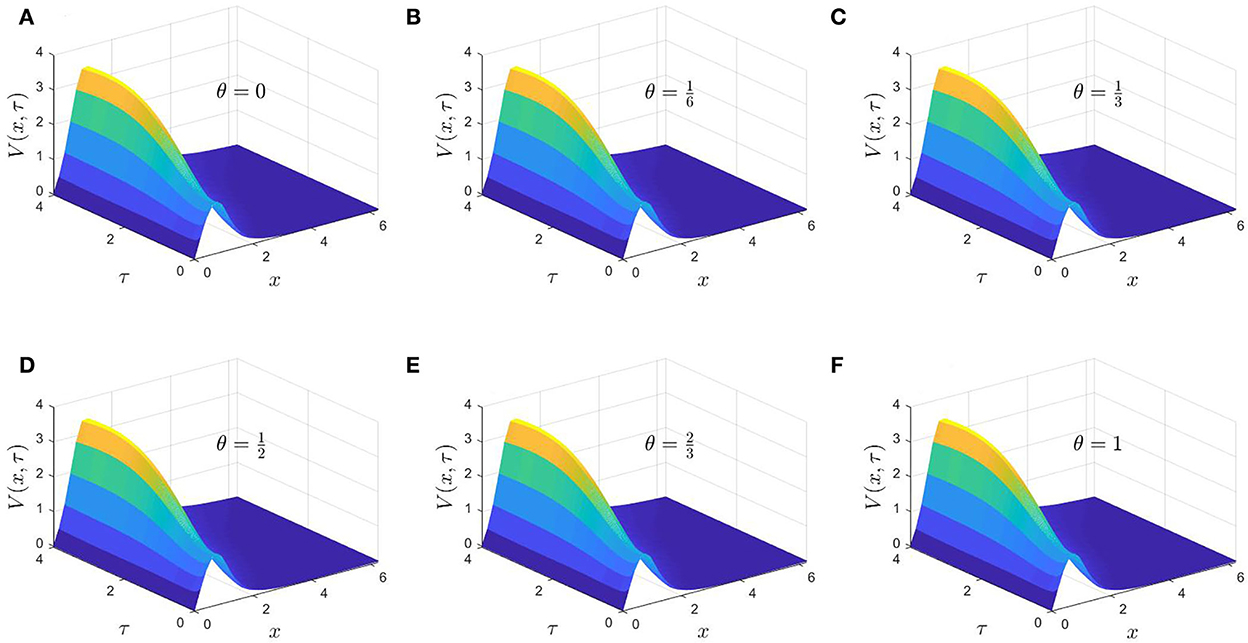
Figure 1. (A–F) The numerical solutions of Example 1 for several values of $\theta \in \left\{0,\frac{1}{6},\frac{1}{3},\frac{1}{2},\frac{2}{3},1\right\}$.

FIGURE 2

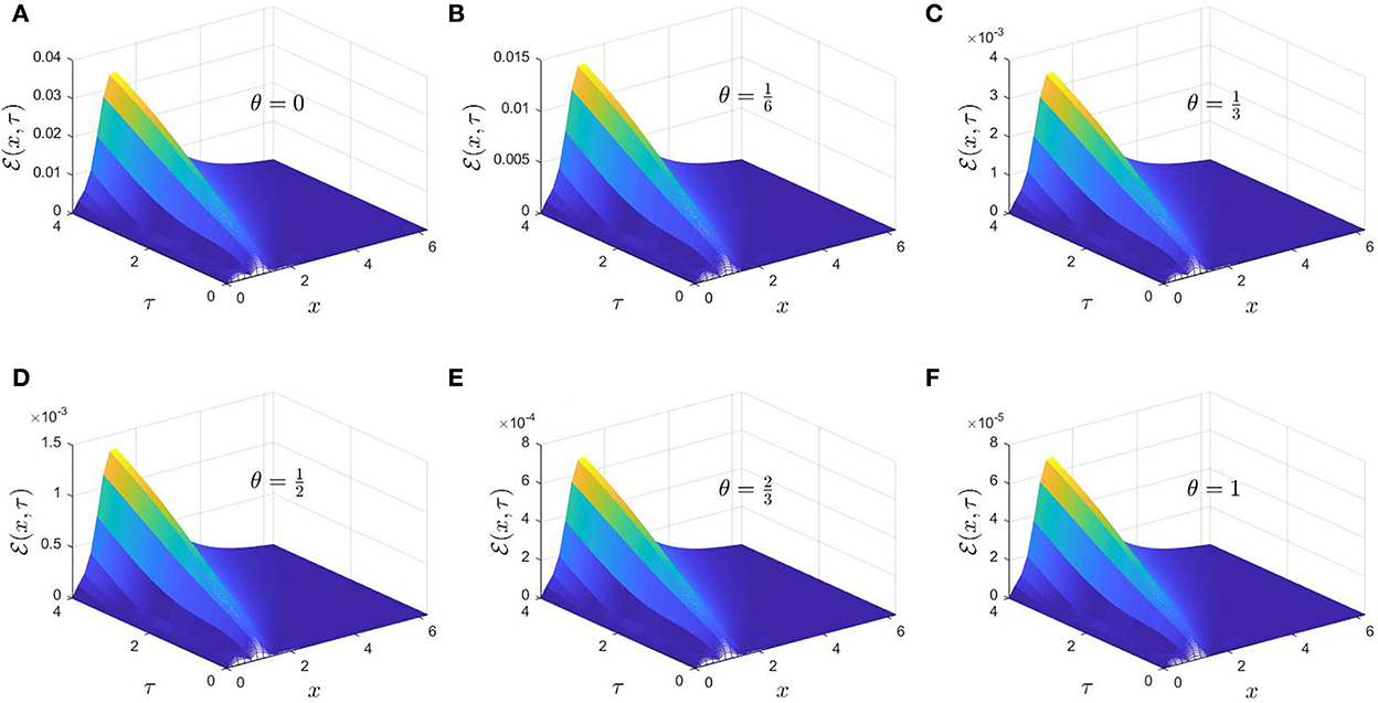
Figure 2. (A–F) The associated absolute error ${E}(x,\tau )$ of Example 1 for each value of θ.

We examine the properties of the maximum absolute error associated with the numerical computations from two aspects; its consistency based on Equation (33) and its convergence rates as the computational domain get finer. First, the order of the consistency of ${{E}}_{max}$ is calculated when (N_x, N_τ) = (32, 256) for each value of the θ-parameter as shown in Table 1 which matches with Equation (33). The maximum absolute error is computed for various mesh grids of (N_x, N_τ); after that, the ratio between two successive maximum errors is calculated to reveal the associated convergence rates as illustrated in Table 2. On the other hand, the order of the absolute error ($ln{E}(x,\tau =T)$) is plotted as a function of the spatial variable x for various values of θ, as shown in Figure 3. The behavior of its order under the explicit, Crank-Nicolson, and fully implicit are grouped in Figure 3A. Figure 3B represents its behavior under the mixed schemes $\theta =\frac{1}{6}$, $\frac{1}{3}$, $\frac{2}{3}$. It has been observed that the maximum error is of order 10⁻³ when x = x_p around the value 1. The computational interval [0, 2π], can be written as the union of two intervals ${\widehat{\Omega }}_p=\left[0,x_p\right]$, and ${\widehat{\Omega }}_p^c=\left[x_p,2\pi \right]$. In the first interval ${\widehat{\Omega }}_p$, the order of error swiftly increases, while it gradually decreases in the second interval ${\widehat{\Omega }}_p^c$, and it reaches to 10⁻⁷, 10⁻⁹, 10⁻¹³ at some points for θ = 0, $\frac{1}{2}$, and 1, respectively as shown in Figure 3A. Moreover, the order of the absolute error significantly decreases as θ increases.

TABLE 1

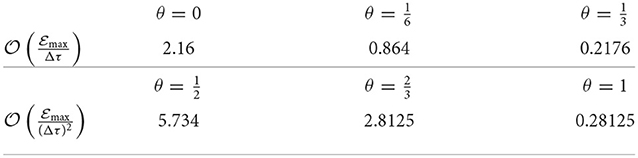
Table 1. The order of the consistency of the absolute maximum errors ${{E}}_{max}$ of Example 1 for all values of θ.

TABLE 2

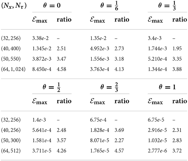
Table 2. The absolute maximum errors for various grids (N_x, N_τ) and their convergence rates for all cases of θ-parameter of Example 1.

FIGURE 3

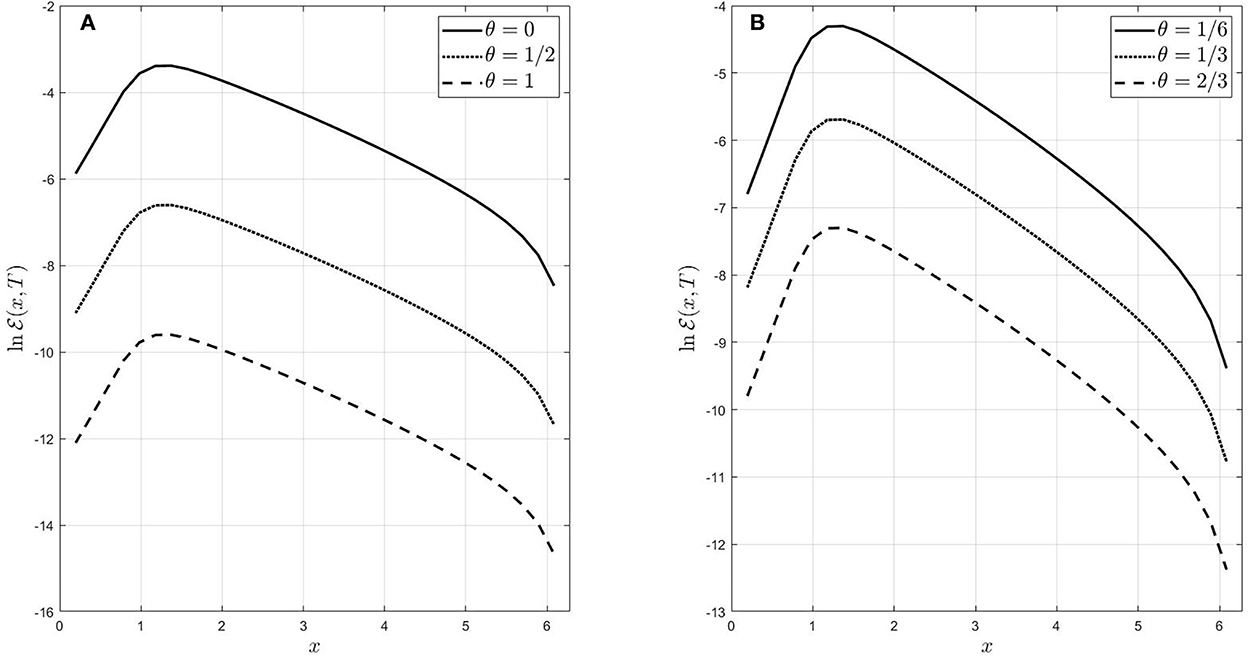
Figure 3. (A,B) The order of absolute error $ln{E}(x,\tau =T)$ for all used finite difference schemes in Example 1.

Next, we discuss the behavior of the associated absolute error (AE) of the proposed finite difference scheme with respect to the change of time-discretization, while the spatial discretization is fixed and vice versa. The absolute errors at x = π/8, 5π/8, 5π/4, and 27π/16 are listed in Table 3 for various values of N_τ together with the corresponding convergence rates β, which is defined by

$\beta =\frac{ln\left(\frac{{{E}}_1}{{{E}}_2}\right)}{ln\left(\frac{N_2}{N_1}\right)},$

and its computational cost in seconds, while the value of N_x is selected as 16. Table 4 is dedicated to revealing the convergence rates and computational cost of the absolute error at τ = 1, 2, 3, 4, due to the change of the number of spatial mesh points N_x, while N_τ remains constant and equals 1,024 for the mixed finite difference scheme $\theta =\frac{1}{6}$, $\frac{1}{3}$, $\frac{2}{3}$.

TABLE 3

Table 3. Absolute errors, their convergence rates, and CPU time for several values of N_τ, while N_x = 16 of Example 1.

TABLE 4

Table 4. Absolute errors, their convergence rates, and CPU time for several values of N_x, when N_τ = 1024 for the problem given in Example 1.

Finally, we investigate the importance of the stability conditions (Equations 27–29). The computational domain is (x, τ) ∈ [0, 2π] × [0, 4], which implies $K=\underset{x,\tau }{\text{max}}\left|{K}(x,\tau )\right|=1$, consequently, we investigate the last condition (Equation 29) for explicit scheme θ = 0, and a mixed scheme $\theta =\frac{1}{3}$. The number of mesh points is selected to be N_x = 16, N_τ = 32, which implies r = 0.81 violates the stability condition

$r\le \{\begin{array}{ll}0.5,& \theta =0.5,\\ 0.75,& \theta =\frac{1}{3}.\end{array}$

On the one hand, Figure 4 represents the surface solution as a function in x, and τ, when the stability condition is broken. On the other hand, Figure 5 shows a cross-section of the solution when τ = T.

FIGURE 4

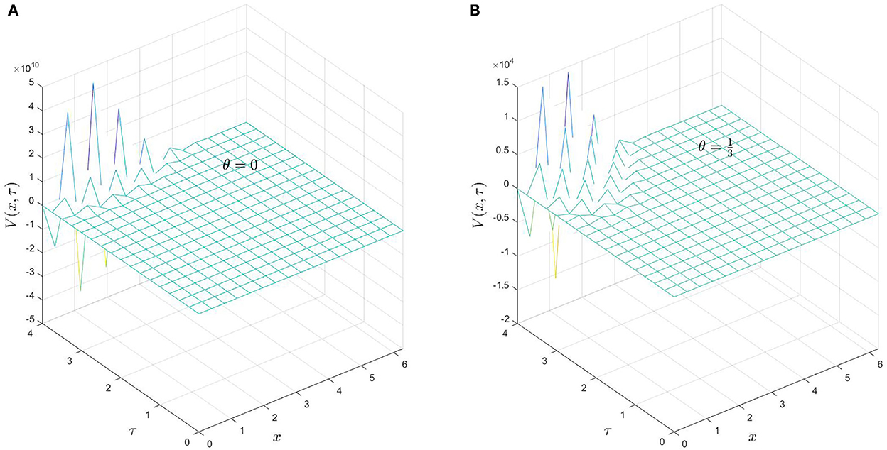
Figure 4. (A,B) The behavior of V(x, τ) of Example 1 when the stability condition (Equation 29) is broken for θ = 0, and $\theta =\frac{1}{3}$.

FIGURE 5

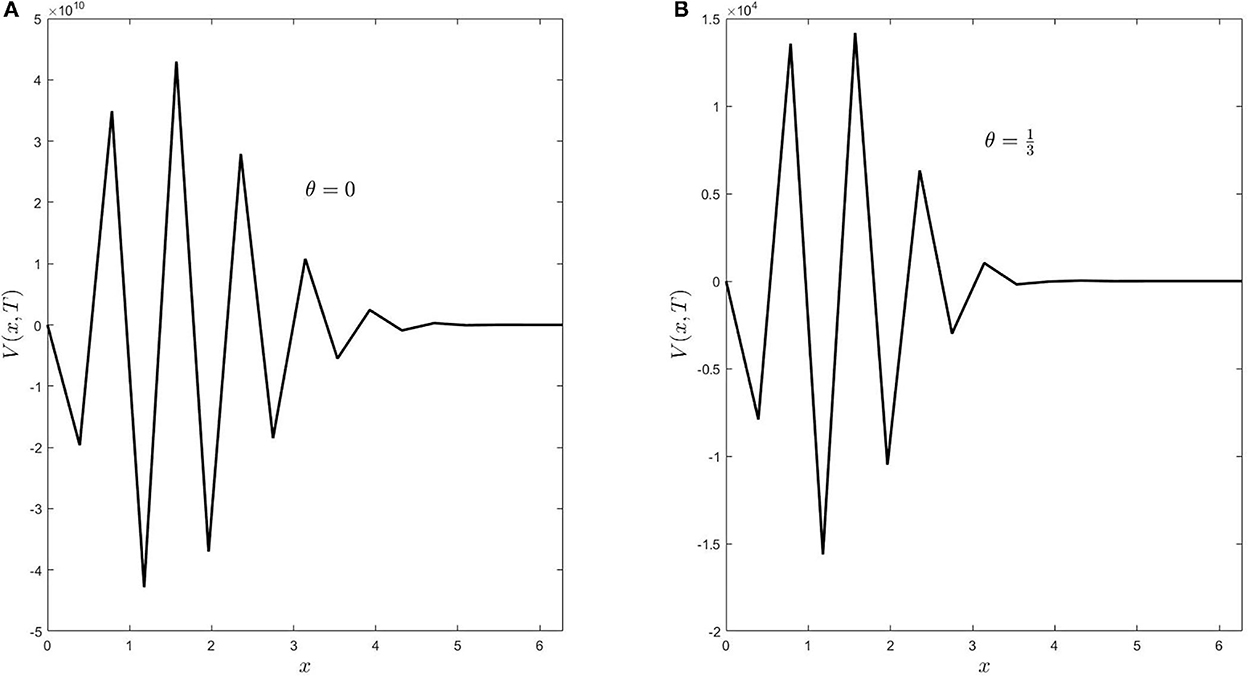
Figure 5. (A,B) The plot of V(x, τ = T) when the stepsizes Δx, and Δτ do not satisfy the stability condition (Equation 29) for θ = 0, and $\theta =\frac{1}{3}$.

Example 2. The goal of this example is to compare the behavior of the proposed finite difference scheme with other techniques, such as the Legendre-collocation method [26]. Problem 1 is chosen [26], where the PIDE problem has kernel ${K}(x,\tau )=e^{x\tau }$, boundary conditions; ${V}(0,\tau )=sin\tau$, ${V}(1,\tau )=0$, and initial condition ${V}(x,0)=0$, and source function

$F(x,\tau )=(1-x^2)cos\tau +2sin\tau -\left(\frac{1-x^2}{1+x^2}\right)(cos\tau +xsin\tau -e^{x\tau }).$

The problem has the exact solution

${V}(x,\tau )=(1-x^2)sin\tau ,x\in \left[0,1\right],\tau \in \left[0,1\right].$

Here, the numerical solutions are obtained for explicit, Crank-Nicolson, and fully implicit cases, also their corresponding absolute errors are calculated for mesh grid points (N_x, N_τ) = (16, 512) as illustrated in Figure 6.

FIGURE 6

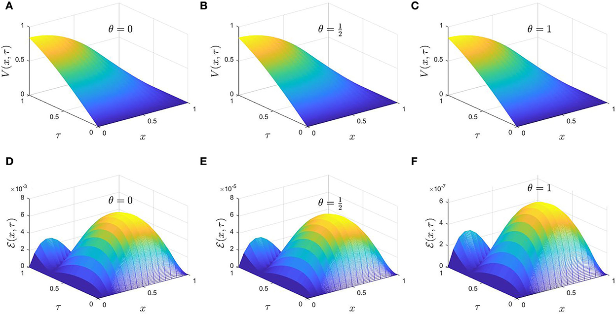
Figure 6. (A–F) The numerical solutions of V(x, τ) of Example 2 for $\theta =0,\frac{1}{2},1$ and their corresponding absolute errors.

For more investigation of the error behavior associated with the computational solutions, we calculate the maximum errors for several grids, the ratios of consecutive ${{E}}_{max}$, and the CPU time as reported in Table 5. It has been observed that for a given mesh grid, the absolute maximum error can be reduced by increasing the value of the θ-parameter. Furthermore, for a given value of θ, the associated error can be reduced by increasing the number of space and time mesh points. However, their increments have different effects; for instance, a modest increase in spatial node number enhances the related error but with a higher computational cost than the same increment in time nodes. Decreasing the space and time stepsizes together leads to second-order convergence. To wrap up, Figure 6 and Table 5 illustrate the performance of the proposed θ-finite difference scheme considering the stability and consistency in solving this problem. On the other hand, the maximum absolute error associated with solving the same problem based on the Legendre-collocation method is available in Table 1 [26, p. 7].

TABLE 5

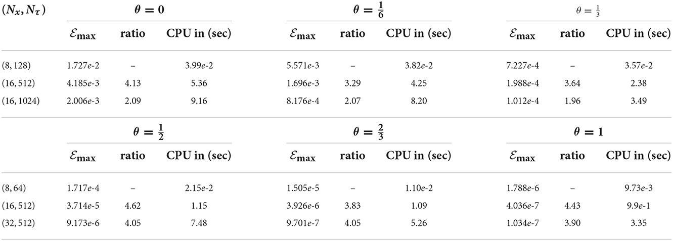
Table 5. The maximum absolute errors, their consecutive ratios, and CPU time for several values of θ of Example 2.

Example 3. This example aims to obtain numerical approximations of a PIDE problem based on the proposed finite difference scheme whose exact solution is unknown. The kernel is ${K}(x,\tau )=e^{x^2{\tau }^2}$, initial and boundary conditions are

${V}(x,0)=x(L-x),{V}(0,\tau )=\frac{\tau }{1+{\tau }^2},{V}(L,\tau )=sin\pi \tau ,$

in the absence of the source function, i.e., F(x, τ) = 0. The computational domain is selected such that $(x,\tau )\in \left[0,\sqrt{6}\right]\times \left[0,1\right]$. Figures 7A–C represent the numerical solutions of explicit, Crank-Nicolson, and fully implicit schemes when the grid nodes (N_x, N_τ) = (16, 128), Figures 7D–F show the corresponding absolute error. To calculate the associated absolute error; a numerical solutions of ${V}(x,\tau )$ are calculated on a refine grid (N_x, N_τ) = (64, 2048), when $\theta =\frac{1}{2}$, and considered as reference values. Consequently, the absolute error is the absolute difference between the corresponding values of $V_k^n$.

FIGURE 7

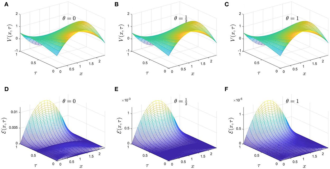
Figure 7. (A–F) The numerical approximations and their absolute errors of Example 3 when $\theta =0,\frac{1}{2},1$.

Next, we discuss the behavior of the errors associated with the numerical solutions by calculating the numerical solutions at five spatial nodes; x = 0.191, 0.612, 0.995, 1.416, and 1.799 using the refine grid (N_x, N_τ) = (64, 2048). After that, the numerical solutions at these points are calculated for various computational grids. Therefore, we calculate so-called the root mean square relative error (RMSRE) such that

$\begin{array}{ll}\text{RMSRE}=\sqrt{\frac{1}{5}{\displaystyle \sum _{i=1}^5}{\left(\frac{V_i^{\text{ref}}(\tau =T)-V_i^{N_{\tau }}}{V_i^{\text{ref}}(\tau =T)}\right)}^2},& (34)\end{array}$

where $V_i^{\mathrm{\text{ref}}}(\tau =T)$, and $V_i^{N_{\tau }}$ are the numerical solutions at the refine grid and the corresponding values of other grids, respectively. Based on these calculations, we present the RMSRE, its ratio of convergence and CPU time in Table 6.

TABLE 6

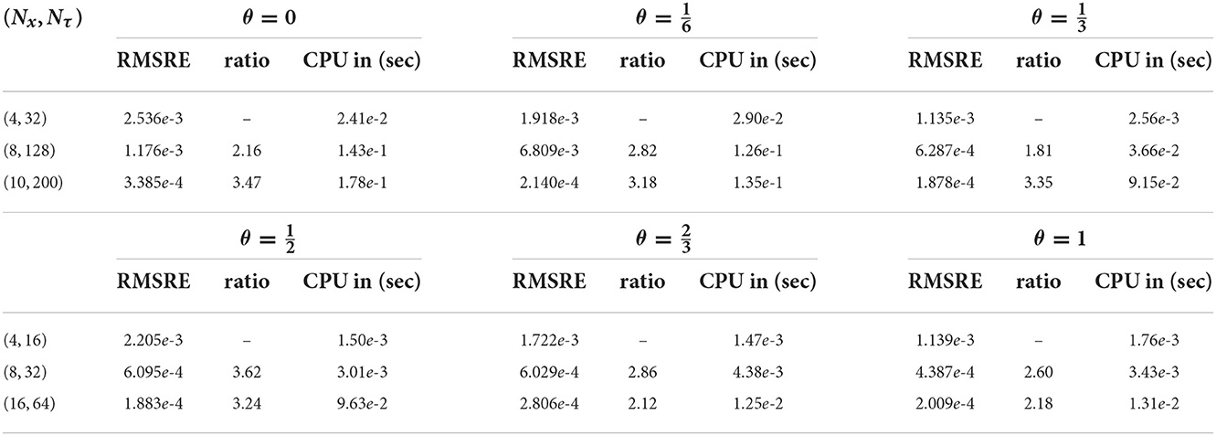
Table 6. The RMSRE of five distinct spatial nods, their ratios, and elapsed time computations for all cases of the θ-parameter of Example 3.

Finally, we show that the stability conditions (Equations 27–29) cannot be neglected. The computational domain $(x,\tau )\in \left[0,\sqrt{6}\right]\times \left[0,1\right]$, consequently, the maximum value of the integral-kernel is K = e⁶ ≈ 403.429 >> 1. So that we investigate the stability condition (Equation 28). Note that it consists of two inequalities; one for the time stepsize and the other for the spatial stepsize. In light of this fact, we consider two cases. The first case is when Δτ satisfies its condition, while the inequality of Δx does not hold. In the second case, when Δτ breaks its inequality, while Δx satisfies its inequality. For the first case, the number of spatial and time nodes are (N_x, N_τ) = (10, 128), then we have

$\Delta x=\frac{L}{N_x}\approx 0.245\Rightarrow K{(\Delta x)}^4=1.452>1,$

consequently, the stability condition (Equation 28) is broken for Δx, while $\Delta \tau =7.8\times 10^{-3}<\frac{1}{\sqrt{K}}=0.0498$. On the one hand, Figure 8 shows the surface of numerical solutions, and a cross-section when τ = T of case one, i.e., Δx, does not satisfy its stability condition. On the other hand, Figure 9 describes the numerical solution behavior under the second case when (N_x, N_τ) = (10, 20) (i.e., $\Delta \tau =0.05>\frac{1}{\sqrt{K}})$. Therefore, stability conditions have a crucial role in obtaining reliable approximations.

FIGURE 8

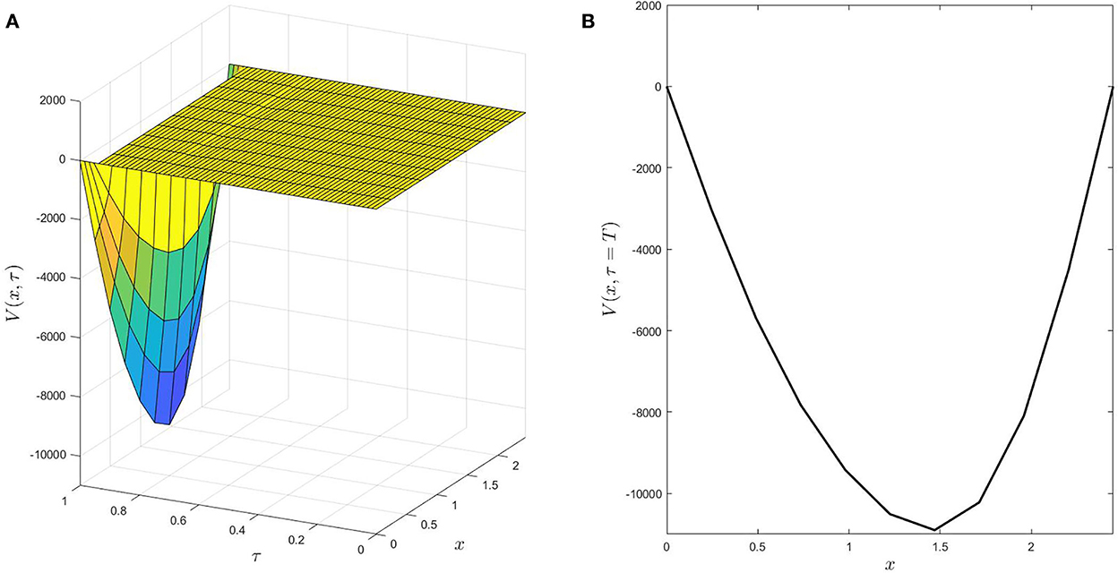
Figure 8. (A,B) The behavior of numerical solutions of Example 3 when the stability condition (Equation 28) is broken with respect to Δx for θ = 0.

FIGURE 9

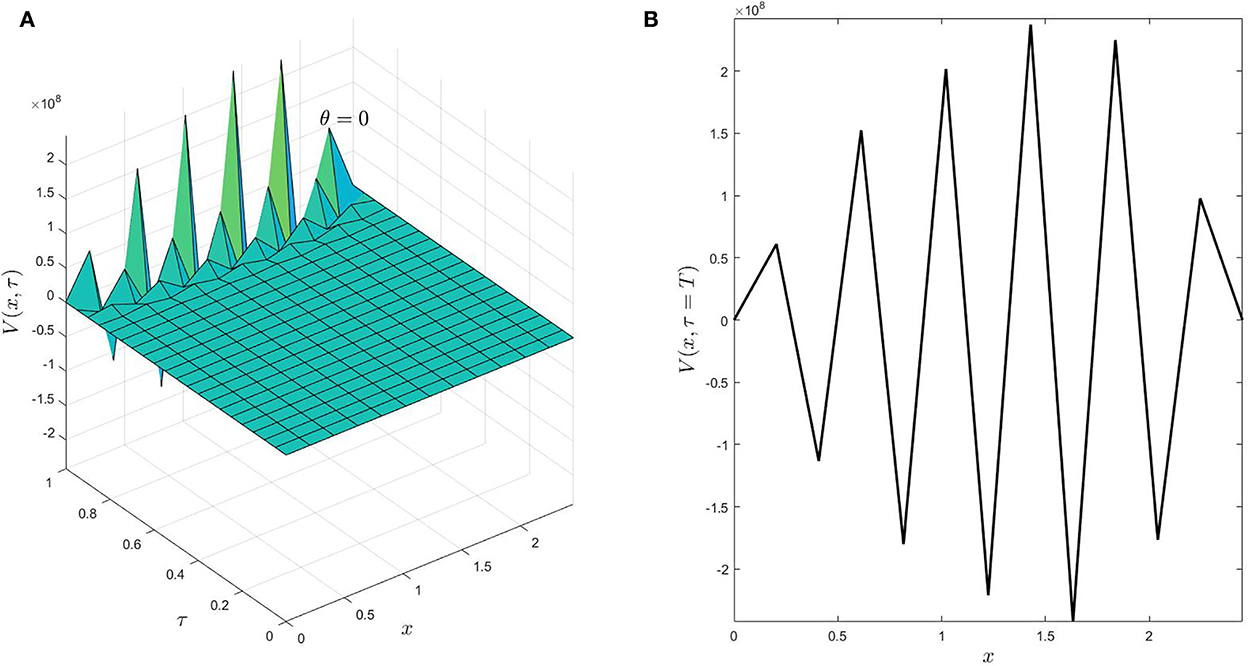
Figure 9. (A,B) A 3D surface of numerical solutions and a 2D-cross section for τ = T when Δτ does not satisfy the stability condition (Equation 28) for θ = 0.

6. Conclusion

The PIDE of memory type has been investigated based on a suitable finite difference scheme. Here the differential part is discretized using the θ-approximation that combines explicit-implicit discretization of the second-order spatial derivative, while the time derivative is approximated using explicit forward discretization. The integral part has two obstacles; first, the upper boundary of the integration is variable, and second, the discretization of an integral part produces more unknowns other than the unknowns of the differential part. We implement the Heaviside step function to convert the upper variable boundary into a constant without changing the independent variables of the unknown function. Consequently, it enables us to discretize it on the same mesh points of the computational domain. The stability of the resulting finite difference scheme has been investigated based on the properties of the matrix norm and Gerschgoren's theorems. Also, consistency has been considered to guarantee the convergence of the numerical approximation. In light of consistency and stability analysis, we have a conditional stable finite difference scheme for θ ∈ [0, 0.5), while it is unconditionally stable for θ ∈ [0.5, 1]. Moreover, it is unconditional consistency. Finally, three examples have been studied to examine the accuracy and stability of the used scheme.

For future research, we will extend the technique used to solve this category of partial integro-differential equations in higher dimensions. Also, we will introduce nonstandard finite difference schemes and investigate their numerical properties.

Data availability statement

The original contributions presented in the study are included in the article/supplementary material, further inquiries can be directed to the corresponding author.

Author contributions

All authors contributed equally to the writing of this paper. Furthermore, all authors also read carefully and approved the final manuscript.

Conflict of interest

The authors declare that the research was conducted in the absence of any commercial or financial relationships that could be construed as a potential conflict of interest.

Publisher's note

All claims expressed in this article are solely those of the authors and do not necessarily represent those of their affiliated organizations, or those of the publisher, the editors and the reviewers. Any product that may be evaluated in this article, or claim that may be made by its manufacturer, is not guaranteed or endorsed by the publisher.

References

1. Yanik EG, Fairweather G. Finite element methods for parabolic and hyperbolic partial integro-differential equations. Nonlinear Anal. (1988) 12:785–809. doi: 10.1016/0362-546X(88)90039-9

CrossRef Full Text | Google Scholar

2. Fakhar-Izadi F, Dehghan M. An efficient pseudo-spectral Legendre-Galerkin method for solving a nonlinear partial integro-differential equation arising in population dynamics. Math Methods Appl Sci. (2013) 36:1485–511. doi: 10.1002/mma.2698

CrossRef Full Text | Google Scholar

3. Fakharany M, Company R, Jódar L. Solving partial integro-differential option pricing problems for a wide class of infinite activity Lévy processes. J Comput Appl Math. (2016) 296:739–52. doi: 10.1016/j.cam.2015.10.027

CrossRef Full Text | Google Scholar

4. Fakharany M, Company R, Jódar L. Positive finite difference schemes for a partial integro-differential option pricing model. Appl Math Comput. (2014) 249:320–32. doi: 10.1016/j.amc.2014.10.064

CrossRef Full Text | Google Scholar

5. Amadori AL. Nonlinear integro-differential evolution problems arising in option pricing: a viscosity solutions approach. Diff Integral Equat. (2003) 16:787–811.

Google Scholar

6. Zappala E, Fonseca AHdO, Moberly AH, Higley MJ, Abdallah C, Cardin J, et al. Neural integro-differential equations. arXiv preprint arXiv:220614282. (2022). doi: 10.48550/arXiv.2206.14282

CrossRef Full Text | Google Scholar

7. Mirzaee F, Rafei Z. The block by block method for the numerical solution of the nonlinear two-dimensional Volterra integral equations. J King Saud Univer Sci. (2011) 23:191–5. doi: 10.1016/j.jksus.2010.07.008

CrossRef Full Text | Google Scholar

8. Mirzaee F, Piroozfar S. Numerical solution of linear Fredholm integral equations via modified Simpson's quadrature rule. J King Saud Univer Sci. (2011) 23:7–10. doi: 10.1016/j.jksus.2010.04.011

CrossRef Full Text | Google Scholar

9. Sakran M. Numerical solutions of integral and integro-differential equations using Chebyshev polynomials of the third kind. Appl Math Comput. (2019) 351:66–82. doi: 10.1016/j.amc.2019.01.030

CrossRef Full Text | Google Scholar

10. Tang T. A finite difference scheme for partial integro-differential equations with a weakly singular kernel. Appl Numer Math. (1993) 11:309–19. doi: 10.1016/0168-9274(93)90012-G

CrossRef Full Text | Google Scholar

11. Xu D. Numerical solution of partial integro-differential equation with a weakly singular kernel based on Sinc methods. Math Comput Simul. (2021) 190:140–58. doi: 10.1016/j.matcom.2021.05.014

CrossRef Full Text | Google Scholar

12. Mirzaee F, Alipour S. Numerical solution of nonlinear partial quadratic integro-differential equations of fractional order via hybrid of block-pulse and parabolic functions. Numer Methods Partial Differ Equ. (2019) 35:1134–51. doi: 10.1002/num.22342

CrossRef Full Text | Google Scholar

13. Fakhar-Izadi F, Dehghan M. The spectral methods for parabolic Volterra integro-differential equations. J Comput Appl Math. (2011) 235:4032–46. doi: 10.1016/j.cam.2011.02.030

CrossRef Full Text | Google Scholar

14. Dehestani H, Ordokhani Y. An efficient approach based on Legendre-Gauss-Lobatto quadrature and discrete shifted Hahn polynomials for solving Caputo-Fabrizio fractional Volterra partial integro-differential equations. J Comput Appl Math. (2022) 403:113851. doi: 10.1016/j.cam.2021.113851

CrossRef Full Text | Google Scholar

15. Yüzbaşı Ş, Yıldırım G. A collocation method to solve the parabolic-type partial integro-differential equations via Pell-Lucas polynomials. Appl Math Comput. (2022) 421:126956. doi: 10.1016/j.amc.2022.126956

CrossRef Full Text | Google Scholar

16. Kumar KH, Vijesh VA. Wavelet based iterative methods for a class of 2D-partial integro differential equations. Comput Math Appl. (2018) 75:187–98. doi: 10.1016/j.camwa.2017.09.008

CrossRef Full Text | Google Scholar

17. Zhu B, Han B, Liu L, Yu W. On the fractional partial integro-differential equations of mixed type with non-instantaneous impulses. Boundary Value Problems. (2020) 2020:1–12. doi: 10.1186/s13661-020-01451-z

CrossRef Full Text | Google Scholar

18. Lakshmikantham V. Theory of Integro-Differential Equations. Vol. 1. Boca Raton, FL: CRC Press (1995).

Google Scholar

19. Smith GD. Numerical Solution of Partial Differential Equations: Finite Difference Methods. Oxford: Oxford University Press (1985).

Google Scholar

20. Linz P. “Analytical and numerical methods for Volterra equations,” in Studies in Applied and Numerical Mathematics. Philadelphia, PA (1985).

Google Scholar

21. Da Fonseca C. On the eigenvalues of some tridiagonal matrices. J Comput Appl Math. (2007) 200:283–6. doi: 10.1016/j.cam.2005.08.047

CrossRef Full Text | Google Scholar

22. Barnett S. Matrices. Methods and Applications. Oxford Applied Mathematics and Computing Science Series. Oxford (1990).

Google Scholar

23. Poole G, Boullion T. A survey on m-matrices. SIAM Rev. (1974) 16:419–27. doi: 10.1137/1016079

CrossRef Full Text | Google Scholar

24. Thomas JW. Numerical Partial Differential Equations: Finite Difference Methods. Vol. 22. New York, NY: Springer Science & Business Media (2013).

Google Scholar

25. Abramowitz M, Stegun IA. Handbook of Mathematical Functions With Formulas, Graphs, and Mathematical Tables. Vol. 55. U.S. Government Printing Office (1964).

Google Scholar

26. Aziz I, Khan I. Numerical solution of partial integrodifferential equations of diffusion type. Math Problems Eng. (2017) 2017:2853679. doi: 10.1155/2017/2853679

CrossRef Full Text | Google Scholar