The transmission dynamics of the monkeypox virus in the presence of environmental transmission

1. Introduction

Monkeypox (MPX) is a contagious zoonotic disease caused by the monkeypox virus (MPXV). It belongs to the genus Orthopoxvirus of the Poxviridae family. MPX is similar to smallpox in clinical presentation and is mostly found in Central and West Africa, which at times spread to other regions, WHO [1] and Jezek et al. [2]. The first identified human MPXV case was a nine-month-old boy in the Democratic Republic of Congo in 1970, WHO [1] and CDC [3]. Afterward, Nigeria had its index case of human MPX in 1971. Thereafter, Nigeria has been experiencing an increasing outbreak of MPXV with over 500 suspected cases that include more than 200 confirmed cases of MPXV, WHO [1]. After the eradication of smallpox globally in 1980, the MPXV has been the leading orthopoxvirus infection in humans to date. In recent times, the reported cases of MPXV infection have greatly increased when compared to the past decades (years), WHO [1], CDC [4], and Nolen et al. [5]. As of 2nd August 2022, there have been a total number of 25,391 MPXV confirmed cases worldwide with 25,047 in non-endemic regions (countries that do not have historically reported cases) and 344 in endemic regions (countries that have historically reported cases), CDC [3]. In addition, between 1 January and 12 June 2022, a total of 141 suspected and 36 confirmed cases of MPXV infection have been reported in Nigeria, NCDC [6]. The main reservoir for MPXV infection in humans is still unknown, but several studies suggested that animals most likely rodents and non-human primates are the potential reservoirs (natural host), WHO [1], CDC [4], and Nolen et al. [5].

The three possible and potential means of transmitting MPXV are animal-human (zoonotic) transmission, human-human transmission, and environmental factors (inter-human or animal) transmission. Animal-human transmission occurs through direct contact with the blood, body fluids, and cutaneous and mucosal lesions of infected animals, WHO [1] and CDC [4]. Zoonotic transmission can occur through the consumption of half-cooked or uncooked meat of these natural hosts, Alakunle et al. [7]. Human to human transmission occurs via close contact with an infected person's bodily fluids, skin lesions or sores, and respiratory tract secretions, WHO [1], CDC [4], and Somma et al. [8]. Transmission via environmental factors occurs when a human or an animal comes into contact with recently infected surfaces or materials contaminated with the virus, whether by infected humans or animals. The MPXV has an incubation period of 7 to 14 days, but this can also range from 5 to 21 days, WHO [1]. Infected persons can spread the virus even before the symptoms appear. In humans, the symptoms of smallpox are more severe and often deadly, as compared to MPXV infection. The obvious symptoms manifested by individuals who may have contracted MPX include fever, severe headache, chills, backache, muscle pain, intense asthenia (fatigue), lymphadenopathy (swollen lymph nodes), followed by a rash and these symptoms last for about 2–4 weeks, WHO [1] and CDC [3]. The lymphadenopathy symptom clinically differentiates MPXV infection from every other member of the Poxviridae family. At present, the case fatality rate (epidemic risk) of MPX is in the range of 3–6% [1].

The main testing mechanism used in the detection of MPXV is the polymerase chain reaction (PCR) or real-time polymerase chain reaction (RT-PCR) blood test. This is the best laboratory test used in the diagnosis of MPX due to its accuracy and sensitivity, WHO [1] and Fowotade et al. [9]. The eradication of MPXV seems complicated and impossible because it infects both humans and animals and there is an increasing encroachment of humans into wildlife habitats where MPX reservoirs are believed to be. In addition, humans do not have direct control over the reservoir of infected animals (animal reservoir). At present, there is no specific or proven treatment or vaccine for MPX, but existing vaccines used for smallpox provides significant protection of approximately 85% efficacy against MPX. In addition, some certain novel antiviral medications, such as Tecovirimat, Brincindofovir, and Vaccinia immune globulin have proven benefits in preventing the spread of infection within the population. It is also worth noting that in 2019, a two-dose vaccine based on a modified attenuated vaccinia virus (Ankara Strain) was approved by WHO for the prevention of MPX, WHO [1]. Under strict and rigorous implementation of infection prevention and control measures, such as the use of PPE (to avoid direct contact with infected persons or animals, and surfaces or materials contaminated with the virus), isolating or quarantining the suspected cases or infected persons, practicing good hand hygiene, raising awareness of the risk factor, use of standard contact and droplet precautions, educating people on the required measures to adopt to reduce the exposure to the MPXV, the probability that the MPXV will lead to an epidemic can be drastically reduced or minimized if these measures are implemented, WHO [1] and CDC [4].

The lack of adequate awareness and knowledge of the transmission dynamics and risk factors of the MPXV disease provides a fertile ground for its spread across both endemic and non-endemic regions. There are not many literature studies on MPXV hence the present unusual outbreak needs urgent research attention into the sudden surge. The reliability of mathematical models has been proven beyond doubt over the years. These efficient mathematical tools have been employed for a better understanding of the potential implications of infectious disease transmission dynamics and for formulating control strategies that suppress and halt the effects of infectious diseases, epidemics, and pandemics, Madubueze et al. [10] and Ogunmiloro [11]. Some scholars have developed mathematical models of MPXV with two interacting host populations, namely the human and non-human (rodent or monkey) populations, Somma et al. [8], Lasisi et al. [12], Usman and Adamu [13], and Emeka et al. [14]. Somma et al. [8] incorporated a public enlightenment campaign parameter and a quarantine class in the human population to control the spread of MPX, while, the exposed class for both human and non-human populations and the vaccination class for migrants were incorporated by Lasisi et al. [12]. Usman and Adamu [13] investigated the effect of combined vaccine and treatment interventions as control strategies to study the transmission dynamics of MPXV infection. Emeka et al. [14], on the other hand, developed a deterministic mathematical model for the transmission dynamics of MPXV, in which they looked at the effect of an imperfect vaccine on the dynamics of infection among the human host population. Their simulations emphasized the impact of a weak, medium, and strong immune system on some epidemiological statuses. Peter et al. [15] established that isolating infected humans will reduce the MPXV in the population. However, MPXV still persists in the population despite the aforementioned results. We, therefore, considered the effect of a contaminated environment (that is surfaces and materials contaminated by MPXV through the shedding of the virus in the environment) on MPXV dynamics. This is based on the epidemiology of MPX, WHO [1] and it forms the motivation of this study. To the best of our knowledge, there have been no studies on MPXV on this. We also include the isolated (quarantined) class [15] and the vaccinated class [13] in the human population. This makes the study to be the first work to consider the impact of quarantine, vaccination, and contaminated environment on the transmission dynamics of MPXV and it describes how the contaminated environment (contaminated surfaces and materials) transmits the infection to the susceptible human population. A quarantine strategy is used to quarantine any suspected cases of MPXV, such that, if the quarantined persons show any signs and symptoms of the MPXV infection, they are isolated for treatment, otherwise, after an incubation period without symptoms, they are moved back to the susceptible class again.

The arrangement of this paper is as follows: Section 2 presents the model formulation for the MPXV, and Sections 3 and 4 discuss the model analysis. Section 5 presents the sensitivity analysis of the formulated model. Section 6 presents numerical simulations to substantiate and validate some analytical results with its discussions, and Section 7 presents the conclusion.

2. Model formulation

There is indeed no perfect mathematical model that can accurately predict the detailed outcome of the infectious disease transmission dynamics, Keeling and Rohani [16] and Ogunmiloro [17]. However, having a thorough understanding of the infectious disease to be modeled is the key to formulating a mathematical model for the disease. Furthermore, when formulating a mathematical model for the infectious disease, it is important to note that as the infection spreads throughout the population, the population is subdivided into non-intersecting compartments, such as susceptible individuals, infected individuals, and recovered individuals. The formulated mathematical model should be able to capture the dynamics of each compartment, taking into account how each compartment changes over time, Martcheva [18].

This section presents the formulation framework for the MPX disease model. During the development of the model, we proposed a compartmental MPX model for the human population (S_H(t), V_H(t), E_H(t), Q_H(t), I_H(t), and R_H(t)), the vector (rodent) population (S_R(t), I_R(t)), and environmental contamination compartment (B(t)). We also considered the following assumptions based on a simplified epidemiological history of the MPXV disease.

• All recruitment (via birth or immigration) into the population is instantly vulnerable to the MPXV disease, WHO [1]

• Susceptible humans can be infected by both infectious rodents and humans, [4]

• Susceptible rodents can be infected by infectious rodents but not by infectious humans, [1] and Marennikova [19]

• Susceptible humans can be infected via MPXV concentration within the environment due to the shedding of the virus by infectious humans and rodents, [4] and Ježek et al. [20]

• Individuals in MPX endemic areas are vaccinated, [1, 8]

• The rodents remain infectious and have no recovered class, WHO [1] and CDC [4]

• All compartments of rodent and human populations are well-mixed, Marennikova and Šeluhina [19]

On the one hand, the total human population at time t, denoted by N_H(t), is subdivided into sub-populations of susceptible (S_H(t)), vaccinated (V_H(t)), exposed (E_H(t)), quarantine (Q_H(t)), infectious, I_H(t), and recovered (R_H(t)) individuals such that N_H(t) = S_H(t)+V_H(t)+E_H(t)+Q_H(t)+I_H(t)+R_H(t). On the other hand, the total rodent population at time t, denoted by N_R(t), is subdivided into sub-populations of susceptible rodents (S_H(t)) and infectious (I_H(t)) rodents such that N_R(t) = S_R(t)+I_R(t).

2.1. Dynamics of the humans

The recruitment of susceptible individuals into the human population occurs via birth or immigration at a constant rate, Λ_H. The susceptible population (S_H(t)) decreased by vaccination of susceptible humans at a rate, ϵ while increased through the loss of vaccine-acquired immunity by vaccinated humans, V_h(t), at a waning rate, ϕ, and through the progression from the quarantine humans, Q_H(t), at a rate, γ. Susceptible humans acquire MPX infection after effective contact with infectious rodents, infectious humans, and contaminated environment, B(t) at a force of infection rate, λ_H is given by

$\begin{array}{l}{\lambda }_H=\frac{{\beta }_1{I}_H}{N_H}+\frac{{\beta }_2{I}_R}{N_R}+\frac{{\beta }_{3}B}{K+B}\end{array}$

where β₁, β₂, and, β₃ are transmission rates from infectious humans to susceptible humans, infectious rodents to susceptible humans, and the concentration of MPXV in the environment to susceptible humans, respectively. The parameter, K, is the concentration of MPX pathogen in the environment which increased by 50% to give rise to MPX transmission and B(t) is the environmental contamination compartment. Natural mortality occurs in all human classes at a rate, μ_H, so that

$\begin{array}{l}\frac{d{S}_H}{dt}={\Lambda }_H-{\lambda }_H{S}_H+\varphi V_H+\gamma Q_H-(\epsilon +{\mu }_H)S_H.\end{array}$

The population of vaccinated humans (V_H(t)) is generated by the vaccination of susceptible individuals at the rate, ϵ. This population decreases due to the waning of the vaccine at the rate, ϕ, and by the natural death rate, μ_H. This gives

$\begin{array}{l}\frac{d{V}_H}{dt}=ϵS_H-(\varphi +{\mu }_H)V_H.\end{array}$

The population of exposed humans (E_H(t)) is formed by the infection of susceptible humans (S_H(t)) at the rate, λ_H. This population is reduced by the progression of individuals to the quarantine and infectious compartments at the rates, σ and τ, respectively, and by the natural death rate, μ_H. Thus,

$\begin{array}{l}\frac{d{E}_H}{dt}={\lambda }_H{S}_H-(\sigma +\tau +{\mu }_H)E_H.\end{array}$

The population of quarantine humans (Q_H(t)) is generated by the progression of exposed humans to the quarantine compartment at a rate, σ. This population also decreases with the progression of quarantine individuals to the susceptible and infectious compartments. The quarantined humans without symptoms after the incubation period return to the susceptible class at a rate, γ, while those with symptoms are isolated for treatment and are progressed to the infected class at a rate, α. This gives,

$\begin{array}{l}\frac{d{Q}_H}{dt}=\sigma E_H-(\gamma +\alpha +{\mu }_H)Q_H.\end{array}$

The population of infectious humans (I_H(t)) is formed by the progression of exposed and quarantine humans to the infectious compartment at the rates, τ and α, respectively. Also, this population decreases through the recovery of the infected humans at the rate, ω, and disease-induced death rate, δ. The infected humans comprise quarantine individuals that develop symptoms and are under treatment and exposed humans who miss the quarantine strategy within the population. This gives,

$\begin{array}{l}\frac{d{I}_H}{dt}=\tau E_H+\alpha Q_H-(\omega +{\mu }_H+\delta )I_H.\end{array}$

The population of recovered humans is generated by the recovery of infectious humans at the rate, ω, and reduces by the natural death at the rate, μ_H, so that

$\begin{array}{l}\frac{d{R}_H}{dt}=\omega I_H-{\mu }_H{R}_H.\end{array}$

2.2. Dynamics of the rodents

The susceptible rodents class, S_R(t), is recruited at a constant rate, Λ_R, and is decreased through acquiring infection following substantial contact with infectious rodents at a rate, λ_R, where,

$\begin{array}{l}{\lambda }_R=\frac{{\beta }_4{I}_R}{N_R}\end{array}$

with β₄ as the transmission rate from infectious rodents to susceptible rodents. It is possible that the susceptible rodents can be infected via interaction with the infected environment. However, this is not considered in this work as the main focus of this study is solely on human interaction with the infected environment. Natural mortality occurs in all rodent compartments at a rate, μ_R. This yields,

$\begin{array}{l}\frac{d{S}_R}{dt}={\Lambda }_R-{\lambda }_R{S}_R-{\mu }_R{S}_R.\end{array}$

The population of infectious rodents, I_R(t), is generated via interaction between the susceptible rodents, (S_R(t)), and infected rodents, (I_R(t)), at the rate, λ_R. This population decreases by a natural death at a rate, μ_R. Hence,

$\begin{array}{l}\frac{d{I}_R}{dt}={\lambda }_R{S}_R-{\mu }_R{I}_R.\end{array}$

2.3. The dynamics of the MPXV concentration within the environment

The concentration of MPXV within the environment is due to the shedding of the virus by infected humans and rodents in the environment, and this contributes to the force of infection, λ_H. There are a number of options in the literature regarding the choice of incidence functions for virus or pathogen interaction in the environment, Hethcote [21], Berge et al. [22], and Tian et al. [23]. For example, Berge et al. [22] showed that the mass action incidence is used for the interaction of Ebola virus in the environment. This study followed Tian and Wang [23]'s approach to cholera infection and formulated the incidence function for the concentration of MPXV in the environment. This is due to the indirect transmission of MPXV that occurs in a saturated manner (how long the virus survives in the environment) and this takes the form

$\begin{array}{l}\frac{{\beta }_{3}B}{K+B}.\end{array}$

The concentration of MPXV in the environment is generated when the infected humans and rodents shed the virus in the environment at the rates, ρ₁andρ₂, respectively. It is reduced by the decay rate of MPXV in the environment at a rate, μ_B. Hence,

$\begin{array}{l}\frac{dB}{dt}={\rho }_1{I}_H+{\rho }_2{I}_R-{\mu }_{B}B.\end{array}$

Thus, the full system of equations for the transmission dynamics of the MPX disease is given by the following nonlinear system of differential equations, and it is presented graphically in Figure 1:

FIGURE 1

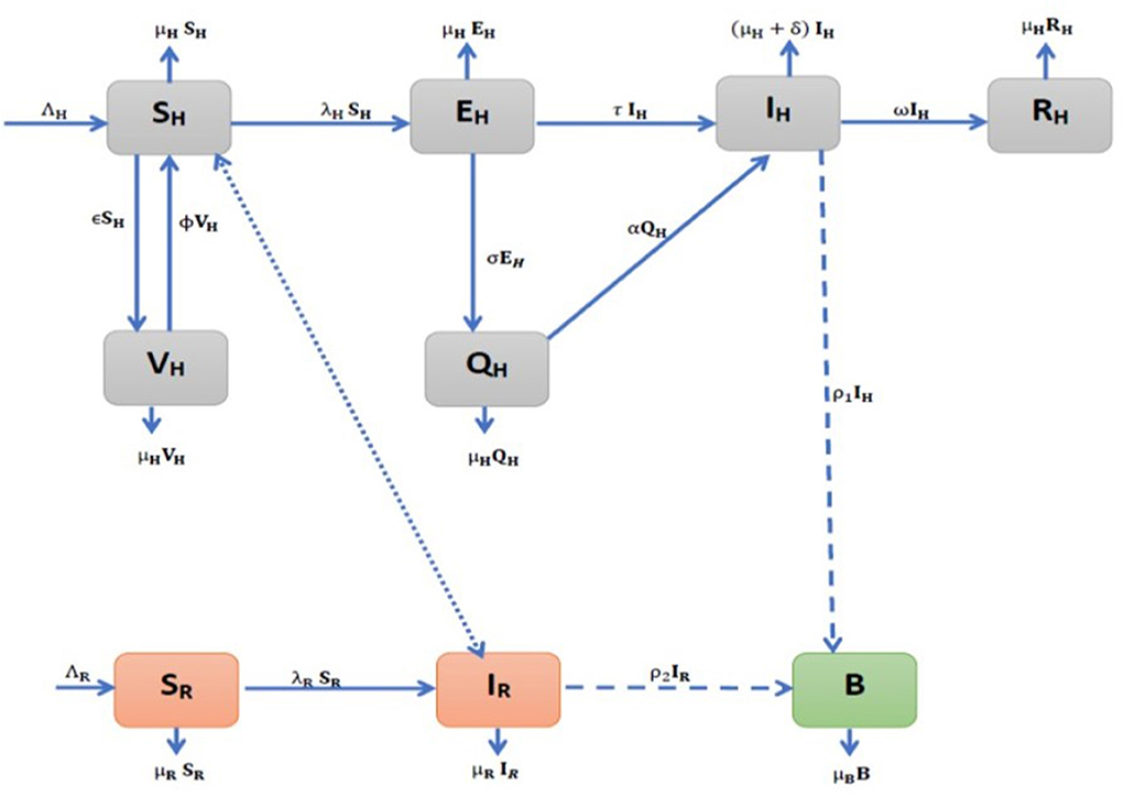
Figure 1. Model flow diagram for the environmental transmission dynamics of Monkeypox (MPX) infection.

$\begin{array}{ll}\frac{d{S}_H}{dt}={\Lambda }_H-{\lambda }_H{S}_H+\varphi V_H+\gamma Q_H-(ϵ+{\mu }_H)S_H,& (1)\end{array}$

$\begin{array}{ll}\frac{d{V}_H}{dt}=ϵS_H-(\varphi +{\mu }_H)V_H,& (2)\end{array}$

$\begin{array}{ll}\frac{d{E}_H}{dt}={\lambda }_H{S}_H-(\sigma +\tau +{\mu }_H)E_H,& (3)\end{array}$

$\begin{array}{ll}\frac{d{Q}_H}{dt}=\sigma E_H-(\gamma +\alpha +{\mu }_H)Q_H,& (4)\end{array}$

$\begin{array}{ll}\frac{d{I}_H}{dt}=\tau E_H+\alpha Q_H-(\omega +{\mu }_H+\delta )I_H,& (5)\end{array}$

$\begin{array}{ll}\frac{d{R}_H}{dt}=\omega I_H-{\mu }_H{R}_H,& (6)\end{array}$

$\begin{array}{ll}\frac{d{S}_R}{dt}={\Lambda }_R-{\lambda }_R{S}_R-{\mu }_R{S}_R,& (7)\end{array}$

$\begin{array}{ll}\frac{d{I}_R}{dt}={\lambda }_R{S}_R-{\mu }_R{I}_R,& (8)\end{array}$

$\begin{array}{ll}\frac{dB}{dt}={\rho }_1{I}_H+{\rho }_2{I}_R-{\mu }_{B}B.& (9)\end{array}$

All state variables are described in Table 1 and are subjected to initial conditions:

TABLE 1

Table 1. Description of state variables.

$\begin{array}{l}{S}_H(0)>0,V_H(0)\ge 0,E_H(0)\ge 0,Q_H(0)\ge 0,I_H(0)\ge 0,\\ R_H(0)\ge 0,S_R(0)>0,I_R(0)\ge 0,B(0)\ge 0.\end{array}$

Also, all the parameters of the MPX model (Equations 1–9) are assumed to be non-negative and are presented in Table 2.

TABLE 2

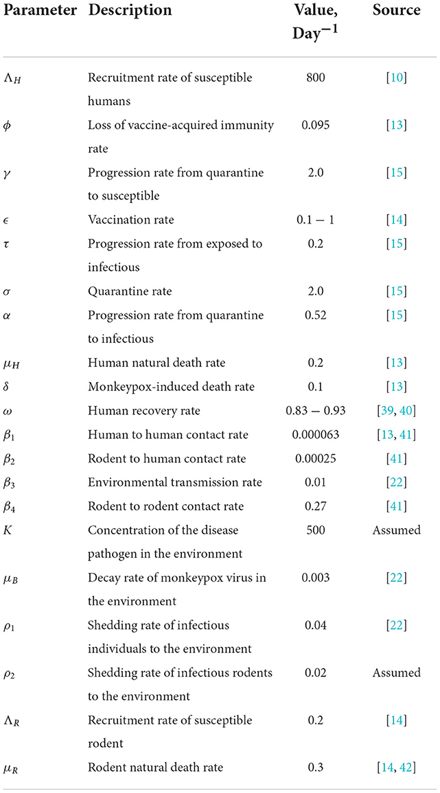
Table 2. Parameter estimation for numerical simulation.

3. Mathematical analysis of model properties

In this section, we quantitatively determined the characteristic properties of the model constituted by establishing the system feasible region and positivity of the system solutions.

3.1. Feasible region

We show that the model system (Equations 1–9) is well-posed by stating and proving the following theorem;

Theorem 3.1. The MPX model (Equations 1–9) is a dynamical system that has a biologically feasible region given as

$\begin{array}{l}\Omega =\{\left(S_H,V_H,E_H,I_H,Q_H,R_H,B\right)\in {ℝ}_{+}^7:\\ 0\le N_H(t)\le \frac{{\Lambda }_H}{{\mu }_H},(S_R,I_R)\in {ℝ}_{+}^2:\\ 0\le N_R(t)\le \frac{{\Lambda }_R}{{\mu }_R},\\ B(t)\le \frac{1}{{\mu }_B}\left(\frac{{\rho }_1{\Lambda }_H}{{\mu }_H}+\frac{{\rho }_2{\Lambda }_R}{{\mu }_R}\right)\}.\end{array}$

Proof: For non-negative initial conditions, the model system (Equations 1–9) possesses at all time, t ≥ 0, a unique non-negative solution that lies in the region, Ω. Following the approaches of Busenberg and Cooke [24] and Stuart and Humphries [25], we add the first six equations of the system (Equations 1–6) such that

$\begin{array}{l}\frac{d{N}_H}{dt}={\Lambda }_H-{\mu }_H{N}_H-\delta I_H\\ \Rightarrow 0\le \frac{d{N}_H}{dt}={\Lambda }_H-{\mu }_H{N}_H-\delta I_H\le {\Lambda }_H-{\mu }_H{N}_H.\end{array}$

Applying Gronwall's inequality implies that

$\begin{array}{l}0\le N_H(t)\le \frac{{\Lambda }_H}{{\mu }_H},\text{ for }0\le N_H(0)\le \frac{{\Lambda }_H}{{\mu }_H},\end{array}$

where N_H(0) is the initial condition of the human population, N_H(t).

Also, by adding the seventh and eighth Equations, we obtain

$\begin{array}{ll}\frac{d{N}_R}{dt}& ={\Lambda }_R-{\mu }_R{N}_R,\end{array}$

which by similar approach yields

$\begin{array}{l}0\le N_R(t)\le \frac{{\Lambda }_R}{{\mu }_R},\text{ for }0\le N_R(0)\le \frac{{\Lambda }_R}{{\mu }_R}.\end{array}$

With I_H ≤ N_H and I_R ≤ N_R, we have from the last equation of the system (Equation 9) that

$\begin{array}{l}\frac{dB}{dt}\le {\rho }_1\left(\frac{{\Lambda }_H}{{\mu }_H}\right)+{\rho }_2\left(\frac{{\Lambda }_R}{{\mu }_R}\right)-{\mu }_{B}B,\end{array}$

which by Gronwall's inequality leads to

$\begin{array}{l}0\le B(t)\le \frac{1}{{\mu }_B}\left\{\frac{{\rho }_1{\Lambda }_H}{{\mu }_H}+\frac{{\rho }_2{\Lambda }_R}{{\mu }_R}\right\},\text{ for }0\le B(0)\\ \le \frac{1}{{\mu }_B}\left\{\frac{{\rho }_1{\Lambda }_H}{{\mu }_H}+\frac{{\rho }_2{\Lambda }_R}{{\mu }_R}\right\}.\end{array}$

Using the well-known result in Theorem 2.1.5 of Stuart and Humphries [25], we conclude that the model system (Equations 1–9) defines a dynamical system within the region, Ω.

3.2. Positivity of the system solutions

We show that all state variables of the MPX dynamics transmission model (Equations 1–9) are non-negative at all time, t > 0, and this means that the model is epidemiologically significant and mathematically well-posed. We state and prove the following theorem:

Theorem 3.2. Let the initial conditions $\left\{S_H(0),V_H(0),E_H(0),Q_H(0),I_H(0),R_H(0),B(0)\ge 0\right\}\in {\Re }_{+}^7$ and $\left\{S_R(0),I_R(0)\ge 0\right\}\in {\Re }_{+}^2$. Then, the solution set {S_H(t), V_H(t), E_H(t), Q_H(t), I_H(t), R_H(t),

S_R(t), I_R(t), B(t)} of the model system (Equations 1–9) is non-negative for all t > 0.

Proof: Using the approach of Madubueze et al. [10], it follows from the first equation of the system (Equations 1–9) that

$\begin{array}{l}\frac{d{S}_H}{dt}={\Lambda }_H-{\lambda }_H{S}_H+\varphi V_H+\gamma Q_H-(\epsilon +{\mu }_H)S_H,\end{array}$

such that

$\begin{array}{l}\frac{d{S}_H}{dt}\ge -{\lambda }_H{S}_H-(\epsilon +{\mu }_H)S_H.\end{array}$

Solving this equation gives

$S_H\ge S_H(0)\exp \left(-{\displaystyle {\int }_0^t{\lambda }_{H}dt}\right)\exp \left(-\left(\epsilon +{\mu }_H\right)t\right)\ge 0$

which is positive, given that S_h(0) is also positive. In the same way,

$\begin{array}{lll}{V}_H(t)& \ge & V_H(0)exp\left\{-(\varphi +{\mu }_H)t\right\}\ge 0,\\ E_H(t)& \ge & E_H(0)exp\left\{-(\sigma +\tau +{\mu }_H)t\right\}\ge 0,\\ Q_H(t)& \ge & Q_H(0)exp\left\{-(\gamma +\alpha +{\mu }_H)t\right\}\ge 0,\\ I_H(t)& \ge & I_H(0)exp\left\{-(\omega +{\mu }_H+\delta )t\right\}\ge 0,\\ R_H(t)& \ge & R_H(0)exp\left\{-{\mu }_{H}t\right\}\ge 0.\end{array}$

It can also be shown for the rodent compartment and the MPX-contaminated environment compartment. This shows that the solution set {S_H(t), V_H(t), E_H(t), Q_H(t), I_H(t), R_H(t), S_R(t), I_R(t), B(t)} is non-negative for all t ≥ 0 since exponential functions and initial solutions are non-negative.

4. The stability analysis of the MPX model

This section presents the quantitative investigation of the model equilibrium states and their stability conditions.

4.1. Monkeypox virus-free equilibrium state (MPXV-FE)

For the existence of an equilibrium state, we require that,

$\begin{array}{l}\frac{d{S}_H}{dt}=\frac{d{V}_H}{dt}=\frac{d{E}_H}{dt}=\frac{d{Q}_H}{dt}=\frac{d{I}_H}{dt}=\frac{d{R}_H}{dt}\\ =\frac{d{S}_R}{dt}=\frac{d{I}_R}{dt}=\frac{dB}{dt}=0,\end{array}$

which implies from the MPX model (Equations 1–9) that

$\begin{array}{l}0={\Lambda }_H-{\lambda }_H{S}_H+\varphi V_H+\gamma Q_H-(ϵ+{\mu }_H)S_H,\\ 0=ϵS_H-(\varphi +{\mu }_H)V_H,\\ 0={\lambda }_H{S}_H-(\sigma +\tau +{\mu }_H)E_H,\\ 0=\sigma E_H-(\gamma +\alpha +{\mu }_H)Q_H,\\ 0=\tau E_H+\alpha Q_H-(\omega +{\mu }_H+\delta )I_H,\\ 0=\omega I_H-{\mu }_H{R}_H,\\ 0={\Lambda }_R-{\lambda }_R{S}_R-{\mu }_R{S}_R,\\ 0={\lambda }_R{S}_R-{\mu }_R{I}_R,\\ 0={\rho }_1{I}_H+{\rho }_2{I}_R-{\mu }_{B}B& (10)\end{array}$

with

$\begin{array}{l}{\lambda }_H=\frac{{\beta }_1{I}_H}{N_H}+\frac{{\beta }_2{I}_R}{N_R}+\frac{{\beta }_{3}B}{K+B}.\end{array}$

and ${\lambda }_R=\frac{{\beta }_4{I}_R}{N_R}.$ Then, from Equation (10), the MPXV-FE for the model (Equations 1–9) exists when there is no infection in the environment, human, and rodent host populations, and it is denoted by E⁰. This implies that there is no infection and thus, no recovery at MPXV-FE, i.e.,

$\begin{array}{l}{E}_H=Q_H=I_H=R_H=I_R=B=0.\end{array}$

Then, we have,

$\begin{array}{l}{E}^0=(S_H^0,V_H^0,E_H^0,Q_H^0,I_H^0,R_H^0,S_R^0,I_R^0,B^0)\end{array}$

$\begin{array}{ll}=\left(\frac{{\Lambda }_{H}q}{pq-\varphi ϵ},\frac{{\Lambda }_Hϵ}{pq-\varphi ϵ},0,0,0,0,\frac{{\Lambda }_R}{{\mu }_R},0,0\right)& (11)\end{array}$

where

$\begin{array}{ll}p=ϵ+{\mu }_H,q=\varphi +{\mu }_H,\text{ and }A=pq-\varphi ϵ={\mu }_H(q+ϵ).& (12)\end{array}$

It is clear from Equation (11) that there is no infection within the human and rodent populations. Now, with the introduction of MPX into the population, it is necessary to investigate the pattern of transmission dynamics. This process invariably requires the computation of the basic reproduction number, which is denoted by ${{R}}_0.$

4.2. Basic reproduction number, ${{R}}_0$

The stability of the disease-free equilibrium, E⁰, is governed and controlled by ${{R}}_0$, which is a crucial mathematical quantity that is considered paramount to the public health sector in the study of the epidemiology of infectious diseases. ${{R}}_0$ is defined as the mean number of secondary infections produced by a single infectious human/rodent when introduced into a completely susceptible population, Diekmann et al. [26]. It is computed using the next-generation approach described by Diekmann et al. [26] with F_i as the rate of new infection and V_i as the rate of transitional terms in the compartment, i. Applying the approach to the MPX model (Equations 1–9) yields

$\begin{array}{l}{F}_i=\left[\begin{array}{c}\frac{{\beta }_1{I}_H}{N_H}+\frac{{\beta }_2{I}_R}{N_R}+\frac{{\beta }_{3}B}{K+B}{S}_H\\ 0\\ 0\\ \frac{{\beta }_4{I}_R{S}_R}{N_R}\\ 0\end{array}\right]and\end{array}$

$\begin{array}{ll}{V}_i=\left[\begin{array}{c}{f}_1{E}_H\\ -\sigma E_H+f_2{Q}_H\\ -\tau E_H-\alpha Q_H+f_3{I}_H\\ {\mu }_R{I}_R\\ -{\rho }_1{I}_H-{\rho }_2{I}_R+{\mu }_{B}B\end{array}\right]& (13)\end{array}$

where i = 1, …, 5 is the number of infected compartments and

$\begin{array}{ll}{f}_1=\sigma +\tau +{\mu }_H,f_2=\gamma +\alpha +{\mu }_H,\text{and}{f}_3=\omega +{\mu }_H+\delta .& (14)\end{array}$

Taking the partial derivatives of F_i and V_i with respect to the infection state variables, E_H, Q_H, I_H, I_R, and B at the MPXV-FE, E⁰ yield the Jacobian matrices

$\begin{array}{l}F=\left[\begin{array}{ccccc}0& 0& \frac{{\beta }_1{S}_H^0}{N_H^0}& \frac{{\beta }_2{S}_H^0}{N_R^0}& \frac{{\beta }_3{S}_H^0}{K}\\ 0& 0& 0& 0& 0\\ 0& 0& 0& 0& 0\\ 0& 0& 0& {\beta }_4& 0\\ 0& 0& 0& 0& 0\end{array}\right]and\end{array}$

$\begin{array}{ll}V=\left[\begin{array}{ccccc}{f}_1& 0& 0& 0& 0\\ -\sigma & f_2& 0& 0& 0\\ -\tau & -\alpha & f_3& 0& 0\\ 0& 0& 0& {\mu }_R& 0\\ 0& 0& -{\rho }_1& -{\rho }_2& {\mu }_B\end{array}\right]& (15)\end{array}$

with $\frac{S_H^0}{N_H^0}=\frac{q}{q+ϵ},$ $\frac{S_H^0}{N_R^0}=\frac{{\mu }_R{\Lambda }_{H}q}{{\mu }_H{\Lambda }_R(q+ϵ)}$, and $S_H^0=\frac{{\Lambda }_{H}q}{A}.$ Hence, FV⁻¹ matrix, where V⁻¹ is the inverse matrix of V, is given by

$\begin{array}{ll}F{V}^{-1}=\left[\begin{array}{ccccc}{k}_1& k_2& k_3& k_4& k_5\\ 0& 0& 0& 0& 0\\ 0& 0& 0& 0& 0\\ 0& 0& 0& \frac{{\beta }_4}{{\mu }_R}& 0\\ 0& 0& 0& 0& 0\end{array}\right]& (16)\end{array}$

where $k_1=\frac{q(\sigma \alpha +f_2\tau )}{f_1{f}_2{f}_3}\left[\frac{{\beta }_3{\Lambda }_H{\rho }_1}{KA{\mu }_B}+\frac{{\beta }_1}{q+ϵ}\right],k_2=\frac{q\alpha }{f_2{f}_3}\left[\frac{{\beta }_1}{q+ϵ}+\frac{{\beta }_3{\Lambda }_H{\rho }_1}{KA{\mu }_B}\right],k_3=\frac{q}{f_3}\left[\frac{{\beta }_1}{q+ϵ}+\frac{{\beta }_3{\Lambda }_H{\rho }_1}{KA{\mu }_B}\right],$ $k_4=\frac{{\Lambda }_{H}q}{{\mu }_R}\left[\frac{{\beta }_3{\rho }_2}{KA{\mu }_B}+\frac{{\beta }_2{\mu }_R}{{\mu }_H{\Lambda }_R(q+ϵ)}\right]$, and $k_5=\frac{{\beta }_3{\Lambda }_{H}q}{KA{\mu }_R}.$ Therefore, ${{R}}_0$ for the MPX model (Equations 1–9) is the spectral radius of the matrix, FV⁻¹, and it is given by

$\begin{array}{l}{{R}}_0=\rho (F{V}^{-1})=max\left[{{R}}_{0R},{{R}}_{0H}\right],\end{array}$

where ${{R}}_{0R}=\frac{{\beta }_4}{{\mu }_R}$ and ${{R}}_{0H}={{R}}_{01}+{{R}}_{02}+{{R}}_{03}+{{R}}_{04}$ with

$\begin{array}{l}{{R}}_{01}=\frac{\alpha \sigma {\beta }_{1}q}{f_1{f}_2{f}_3(q+ϵ)},{{R}}_{02}=\frac{{\beta }_{1}q\tau }{f_1{f}_2(q+ϵ)},\\ {{R}}_{03}=\frac{{\Lambda }_H{\beta }_3{\rho }_{1}q\alpha \sigma }{AK{f}_1{f}_2{f}_3{\mu }_B},\text{ and }{{R}}_{04}=\frac{{\Lambda }_H{\beta }_3{\rho }_{1}q{f}_2\tau }{AK{f}_1{f}_3{\mu }_B}.\end{array}$

Here, R_0R and R_0H are the reproduction numbers for rodent to rodent transmission and human-human and environment transmission respectively. The reproduction numbers R₀₁ and R₀₂ are for human-human transmission while R₀₃ and R₀₄ are reproduction numbers for human-environmental contact.

The biological insight by Diekmann et al. [26] indicates that the MPXV infection can be eliminated in both human and rodent host populations if ${{R}}_0<1$, while it can persist in both host populations when ${{R}}_0>1$.

4.3. Local stability of MPX-FE

The local stability of the MPX-FE state, E⁰, of the model (Equations 1–9) is established in terms of ${{R}}_0$ by determining the eigenvalues of linearized Jacobian matrix, J(E⁰), that is evaluated at E⁰.

Theorem 4.1. The monkeypox-free equilibrium, E⁰, of model system (Equations 1–9) is locally asymptotically stable if ${{R}}_0=max\left[{{R}}_{0R},{{R}}_{0H}\right]<1$, otherwise it is unstable.

Proof: To prove the local stability of the MPXV-FE, E⁰, we show that the Jacobian matrix, J(E⁰), of the model system (1–9) at E⁰ has negative eigenvalues. The Jacobian matrix, J(E⁰), is given by

$\begin{array}{ll}J(E^0)=\left[\begin{array}{ccccccccc}-p& \varphi & 0& \gamma & -\frac{{\beta }_1{S}_H^0}{N_H^0}& 0& 0& -\frac{{\beta }_2{S}_H^0}{N_R^0}& -\frac{{\beta }_3{S}_H^0}{K}\\ ϵ& -q& 0& 0& 0& 0& 0& 0& 0\\ 0& 0& -f_1& 0& \frac{{\beta }_1{S}_H^0}{N_H^0}& 0& 0& \frac{{\beta }_2{S}_H^0}{N_R^0}& \frac{{\beta }_3{S}_H^0}{K}\\ 0& 0& \sigma & -f_2& 0& 0& 0& 0& 0\\ 0& 0& \tau & \alpha & -f_3& 0& 0& 0& 0\\ 0& 0& 0& 0& \omega & -{\mu }_H& 0& 0& 0\\ 0& 0& 0& 0& 0& 0& -{\mu }_R& -{\beta }_4& 0\\ 0& 0& 0& 0& 0& 0& 0& {\beta }_4-{\mu }_R& 0\\ 0& 0& 0& 0& {\rho }_1& 0& 0& {\rho }_2& -{\mu }_B\end{array}\right].& (17)\end{array}$

The eigenvalues of J(E⁰) are −μ_R, β₄ − μ_R, and −μ_H and the solutions of the 6th-degree polynomial that is given by

$\begin{array}{ll}{{D}}_0{\lambda }^6+{{D}}_1{\lambda }^5+{{D}}_2{\lambda }^4+{{D}}_3{\lambda }^3+{{D}}_4{\lambda }^2+{{D}}_5\lambda +{{D}}_6=0.& (18)\end{array}$

Here, the coefficients D_i(i = 0, 1, 2, …, 5) are defined in terms of reproduction numbers, ${{R}}_{01},{{R}}_{02},{{R}}_{03}$, ${{R}}_{04}$, and R_0H as

$\begin{array}{l}{{D}}_0=1,\\ {{D}}_1={\mu }_B+f_1+f_2+f_3+p+q,\\ {{D}}_2=pq-\varphi \epsilon +(p+q)(f_1+f_2+f_3+{\mu }_B)+f_1{f}_3(1-{ℛ}_{02})\\ +(f_2+{\mu }_B)(f_1+f_3)+{\mu }_B{f}_2,\\ {{D}}_3=f_1{f}_2{f}_3(1-{ℛ}_{0H})+(pq-\varphi \epsilon )(f_1+f_2+f_3+{\mu }_B)\\ +(p+q)(f_1{f}_2+f_1{f}_3+f_1{\mu }_B+f_2{f}_3+f_2{\mu }_B+f_3{\mu }_B)\\ +f_1{f}_3{\mu }_B(1-{ℛ}_{02}-{ℛ}_{04})+f_2{\mu }_B(f_1+f_3),\\ {{D}}_4=(pq-\varphi \epsilon )[f_1{f}_2+f_1{\mu }_B+f_2{f}_3+f_2{\mu }_B+f_3{\mu }_B\\ +f_1{f}_3(1-{ℛ}_{02})]+f_1{f}_2{f}_3{\mu }_B(1-{ℛ}_{0H})\\ +f_1{f}_2{f}_3(p+q)(1-{ℛ}_{01}-{ℛ}_{02})\\ +f_1{f}_3(p+q){\mu }_B(1-{ℛ}_{02}-{ℛ}_{04})+f_2{\mu }_B(f_1+f_3)(p+q),\\ {{D}}_5=f_1{f}_2{f}_3{\mu }_B(p+q)(1-{ℛ}_{0H})+(pq-\varphi \epsilon )\\ f_1{f}_2{f}_3(1-{ℛ}_{01}-{ℛ}_{02})+(pq-\varphi \epsilon ){\mu }_B{f}_1\\ f_3(1-{ℛ}_{02}-{ℛ}_{04})+(pq-\varphi \epsilon )f_2{\mu }_B(f_1+f_3),\text{ and}\\ {{D}}_6=(pq-\varphi \epsilon ){\mu }_B{f}_1{f}_2{f}_3(1-{ℛ}_{0H}).\end{array}$

Using the Routh-Hurwitz criteria in Kim et al. [27] and conditions in Heffernan et al. [28] that if the inequalities

$\begin{array}{l}{{D}}_i>0(i=0,1,2,\dots ,6),{{D}}_1{{D}}_2>{{D}}_0{{D}}_3,\\ {{D}}_4{{D}}_5>{{D}}_3{{D}}_6,{{D}}_2{{D}}_4>{{D}}_6{{D}}_0,\end{array}$

are satisfied, then the polynomial (Equation 18) has negative real part solutions. This is true provided ${{R}}_0<1.$ Hence, the MPXV-FE, E⁰, is locally asymptotically stable if ${{R}}_0=max\left[R_{0R},R_{0H}\right]<1$, since β₄ − μ_B = μ_R(R_0R − 1) and R_0H = R₀₁ + R₀₂ + R₀₃ + R₀₄, otherwise it is unstable when ${{R}}_0>1.$ Theorem (3) means that the MPXV will be eradicated in the population provided R₀ < 1.

4.4. Existence of endemic equilibrium (EE) states

The model (Equations 1–9) achieves the endemic equilibrium state when the monkeypox disease persists within the population that is when at least one of the infected state variables of the system (Equations 1–9) is not equal to zero. There are two endemic equilibria, namely the infected-rodent-free endemic equilibrium (IRF-EE) and the coexistence endemic equilibrium (CO-EE). Solving simultaneously the rodent compartments of the system (Equation 9) yields $S_R^0=\frac{{\Lambda }_R}{{\mu }_R},I_R^0=0$ for IRF-EE and $S_R^{*}=\frac{{\Lambda }_R}{{\beta }_4},I_R^{*}=\frac{{\Lambda }_H(R_{0R}-1)}{{\beta }_4}$, for CO-EE.

4.4.1. Infected rodent-free endemic equilibrium

Theorem 4.2. There exists a unique IRF-EE when ${{R}}_{0H}>1$ for the model system (Equations 1–9).

Proof: Solving simultaneously the human host and environmental compartments of the Equation (10) in terms of ${\lambda }_H^{*}=\frac{{\beta }_1{I}_H}{N_H}+\frac{{\beta }_{3}B}{K+B}$ for $S_R^0=\frac{{\Lambda }_R}{{\mu }_R},I_R^0=0$, we have IRF-EE, $E_{IRF}^{*}=(S_H^{*},V_H^{*},E_H^{*},Q_H^{*},I_H^{*},R_H^{*},\frac{{\Lambda }_R}{{\mu }_R}$,0, B^*)

where

$\begin{array}{l}{S}_H^{*}=\frac{f_1{f}_{2}q{\Lambda }_H}{{\lambda }_H^{*}q(f_1{f}_2-\gamma \sigma )+f_1{f}_{2}A},\\ V_H^{*}=\frac{ϵf_1{f}_2{\Lambda }_H}{{\lambda }_H^{*}q(f_1{f}_2-\gamma \sigma )+f_1{f}_{2}A},\\ E_H^{*}=\frac{q{f}_2{\Lambda }_H{\lambda }_H^{*}}{{\lambda }_H^{*}q(f_1{f}_2-\gamma \sigma )+f_1{f}_{2}A},\\ Q_H^{*}=\frac{q\sigma {\Lambda }_H{\lambda }_H^{*}}{{\lambda }_H^{*}q(f_1{f}_2-\gamma \sigma )+f_1{f}_{2}A},\\ I_H^{*}=\frac{q{\Lambda }_H(\tau f_2+\alpha \sigma ){\lambda }_H^{*}}{f_3\left[{\lambda }_H^{*}q(f_1{f}_2-\gamma \sigma )+f_1{f}_{2}A\right]},\\ R_H^{*}=\frac{\omega q{\Lambda }_H(\tau f_2+\alpha \sigma ){\lambda }_H^{*}}{{\mu }_H{f}_3\left[{\lambda }_H^{*}q(f_1{f}_2-\gamma \sigma )+f_1{f}_{2}A\right]},\\ \text{and}\\ B^{**}=\frac{{\rho }_{1}q{\Lambda }_H(\tau f_2+\alpha \sigma ){\lambda }_H^{*}}{{\mu }_B{f}_3\left[{\theta }_H^{**}q(f_1{f}_2-\gamma \sigma )+f_1{f}_{2}A\right]},& (19)\end{array}$

with ${\lambda }_H^{*}=0$ and ${\lambda }_H^{*}$ as the solution of

$\begin{array}{ll}{{M}}_2{\lambda }_H^{*2}+{{M}}_1{\lambda }_H^{*}-{{M}}_0=0,& (20)\end{array}$

such that

$\begin{array}{l}{{M}}_2=q^{2}GH,\\ {{M}}_1={\mu }_H{f}_1{f}_2{f}_{3}q(q+ϵ)(1-{{R}}_{01}-{{R}}_{02})G\\ +{\mu }_{B}AK{f}_1^2{f}_2^2{f}_3^{2}H(1-R_{03}-{{R}}_{04}),\\ {{M}}_0={\mu }_H{\mu }_{B}AK{f}_1^2{f}_2^2{f}_3^2(q+ϵ)({{R}}_{0H}-1),& (21)\end{array}$

where

$\begin{array}{l}G={\Lambda }_H{\rho }_1(\alpha \sigma +f_2\tau )+{\mu }_{B}K{f}_3(f_1{f}_2-\gamma \sigma ),\\ H=f_3{\mu }_H(f_2+\sigma )+({\mu }_H+\omega )(\alpha \sigma +f_2\tau ),& (22)\end{array}$

and f₁f₂ − γσ > 0.

Here, ${\lambda }_H^{*}=0$ corresponds to the MPX disease-FE, E⁰, in Equation (11) while the positive solution of Equation (20), ${\lambda }_H^{*}=\frac{-{{M}}_1+\sqrt{{{M}}_1^2+4{{M}}_2{{M}}_0}}{2{{M}}_2}$ represents IRF-EE, $E_{IRF}^{**}$, of the model system (Equations 1–9) and hence ${\lambda }_H^{*}>0$ provided ${{R}}_{0H}>1.$ This gives a forward bifurcation at ${{R}}_{0H}=1$ in the absence of infected rodents and it showed graphically in Figure 2.

FIGURE 2

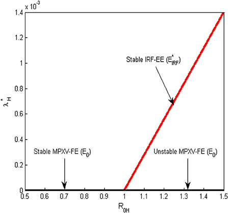
Figure 2. Forward bifurcation plot for the transmission dynamics of the MPX infection at the human-human and environment reproduction number (${{R}}_{0H}$) = 1.

4.4.2. Coexistence endemic equilibrium state

The coexistence endemic equilibrium state of model system (Equations 1–9) occurs when $S_R^{*}=\frac{{\Lambda }_R}{{\beta }_4},I_R^{*}=\frac{{\Lambda }_H(R_{0R}-1)}{{\beta }_4}$, and it is denoted as $E_{C0}^{*}=(S_H^{*},V_H^{*},E_H^{*},Q_H^{*},I_H^{*},R_H^{*},\frac{{\Lambda }_R}{{\beta }_4},\frac{{\Lambda }_H(R_{0R}-1)}{{\beta }_4},B^{*}).$ Solving simultaneously the human host, rodent host, and environmental compartments at equilibrium state in terms of ${\lambda }_H^{**}=\frac{{\beta }_1{I}_H}{N_H}+\frac{{\beta }_2{I}_R}{N_R}+\frac{{\beta }_{3}B}{K+B}$ for $S_R^{*}=\frac{{\Lambda }_R}{{\beta }_4},I_R^{*}=\frac{{\Lambda }_H(R_{0R}-1)}{{\beta }_4},$ we obtain the polynomial

$\begin{array}{ll}{{E}}_3{\lambda }_H^{**3}+{{E}}_2{\lambda }_H^{**2}+{{E}}_1{\lambda }_H^{**}+{{E}}_0=0,& (23)\end{array}$

where

$\begin{array}{l}{{E}}_3=q^{2}HQ,\\ {{E}}_2=\left[1-{{R}}_{01}-{{R}}_{02}\right]{\mu }_H{f}_1{f}_2{f}_{3}q(q+ϵ)Q\\ +(1-{{R}}_{03}-{{R}}_{04}){\mu }_{B}AK{f}_1{f}_2{f}_{3}qH\\ +\frac{A{\Lambda }_R({{R}}_{0R}-1)f_1{f}_2{f}_{3}q{\rho }_{2}H}{{\beta }_4}\\ \times \left[1-\frac{{\beta }_3(f_1{f}_2-\gamma \sigma )q}{A{f}_1{f}_2}\right]+{\beta }_2{\mu }_R(1-{{R}}_{0R})q^{2}QH,\\ {{E}}_1={\beta }_2{\mu }_R(1-{{R}}_{0R})f_1{f}_2{f}_{3}Z\\ +\frac{{\beta }_{3}A{\Lambda }_R(1-{{R}}_{0R})f_1{f}_2{f}_{3}q{\rho }_{2}H}{{\beta }_4}+(1-{{R}}_{0H}){\mu }_H{\mu }_B\\ \times AK{f}_1^2{f}_2^2{f}_3^2(q+ϵ)\\ +\frac{{\mu }_{H}A{\Lambda }_R(1-{{R}}_{0R})f_1^2{f}_2^2{f}_3^{2}q{\rho }_2(q+ϵ)}{{\beta }_4}\\ \times \left[{{R}}_{01}+{{R}}_{02}+\frac{{\beta }_3(f_1{f}_2-\gamma \sigma )q}{A{f}_1{f}_2}-1\right],\\ {{E}}_0=(1-{{R}}_{0R}){\mu }_{H}A{f}_1^2{f}_2^2{f}_3^2(q+ϵ)M,& (24)\end{array}$

with

$\begin{array}{l}Q=G+\frac{{\Lambda }_R(f_1{f}_2-\gamma \sigma )f_3{\rho }_2({{R}}_{0R}-1)}{{\beta }_4},\\ M=\frac{{\beta }_3{\rho }_2{\Lambda }_R}{{\beta }_4}+{\beta }_2{\mu }_{B}K{\mu }_R+\frac{{\beta }_2{\Lambda }_R{\mu }_R({{R}}_{0R}-1){\rho }_2}{{\beta }_4},\\ \text{ and}\\ Z=AqH\left[\frac{{\Lambda }_R({{R}}_{0R}-1){\rho }_2}{{\beta }_4}+{\mu }_{B}K\right]+{\mu }_H(q+ϵ)Q.& (25)\end{array}$

Note that the state variables of co-existence equilibrium, $S_H^{*},V_H^{*},E_H^{*},Q_H^{*},I_H^{*},R_H^{*},\mathrm{\text{and}}{B}^{*}$ are defined in Equation (19) with ${\lambda }_H^{*}$ in Equation (20) as ${\lambda }_H^{**}$ in Equation (23).

Theorem 4.3. For the monkeypox model (Equations 1–9), there exists a positive unique CO-EE when ${{R}}_{0R}>1,$ and it exhibits a backward bifurcation at ${{R}}_{0R}=1$ if ${{E}}_2>(<)0$ and ${{E}}_1<0$ or ${{E}}_2<0$ and ${{E}}_1>0$, otherwise a backward bifurcation does not exist when ${{E}}_2>0$ and ${{E}}_1>0.$

Proof: The number of positive roots of Equation (23) is determined by the signs of its coefficients using Descartes' rule of signs. If ${{R}}_{0R}>1$, it implies that the coefficients, ${{E}}_3>0$ and ${{E}}_0<0.$ The signs of ${{E}}_2$ and ${{E}}_1$ are determined by ${{R}}_{0H}$ such that when ${{R}}_{0H}<1$ or ${{R}}_{0H}>1$, Equation (23) has a unique positive equilibrium. Hence, a positive CO-EE, $E_{CO}^{*}$, exists if ${{R}}_{0R}>1.$

Furthermore, when ${{R}}_{0R}$ is < 1, ${{E}}_0>0$ and ${{E}}_3>0$ with the assumption that Q > 0. The signs of ${{E}}_2$ and ${{E}}_1$ are determined using Descartes rule of signs such that if ${{E}}_2>(<)0$ and ${{E}}_1<0$ or ${{E}}_2<0$ and ${{E}}_1>0$, two EE exist for ${{R}}_{0R}$ < 1. However, when ${{E}}_2>0$ and ${{E}}_1>0,$ no positive endemic equilibrium exists for ${{R}}_{0R}<1.$ Therefore, the MPX model (Equation 18) has two positive equilibria that coexist with MPXV-FE, E⁰, when ${{R}}_{0R}$ < 1 which implies the presence of backward bifurcation at ${{R}}_{0R}=1.$ The backward bifurcation plot for the MPX model (Equations 1–9) at ${{R}}_{0R}=1$ is displayed in Figure 3. Note that the backward bifurcation exists only at ${{R}}_{0R}=1$ which involves the coexistence of the two populations and their respective reproduction numbers.

FIGURE 3

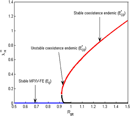
Figure 3. Backward bifurcation plot for the transmission dynamics of the MPX infection at the rodent-rodent reproduction number (${{R}}_{0R}$) = 1.

4.5. Global stability of the equilibrium states

We present in this subsection, the global stability of the equilibrium states. To begin, we state the following notations.

Lemma 4.4. From Bassey et al. [29] and Chien and Shateyi [30], let A > 0 (< 0) be a real square matrix of order n. If A is symmetric positive (negative) definite, then all the eigenvalues of A have negative (positive) real parts if and only if there exists a matrix H > 0 such that

$HA+A^T{H}^T<0(>0).$

Lemma 4.5. Using the global stability theorem in Castillo-Chavez et al. [31], consider a disease model system written in the form

$\begin{array}{l}\frac{dX}{dt}=F(X,Z),\\ \frac{dZ}{dt}=G(X,Z)\end{array}$

with G(X, 0) = 0, where X ∈ R^m and Z ∈ Rⁿ represent uninfected and infected sub-populations (compartments), respectively. $X_0=(X^t,0)$ denotes the disease-free equilibrium of the model.

Assuming that the following conditions hold:

1. $\frac{dX}{dt}=F(X,0),X^t$ is globally asymptotically stable.

2. G(X, Z) = AZ − Ĝ(X, Z) with Ĝ(X, Z) ≥ 0 for all (X, Z) ∈ Ω, where Jacobian matrix $A=\frac{\partial G}{\partial Z}(X^t,0)=F-V$ is an M-matrix, whose off-diagonal elements are negative. Then, the disease-free equilibrium, DFE $X_0=(X^t,0)$ is globally asymptotically stable if R₀ < 1.

Lemma 4.6. From Bassey and Atsu [29] and Chien and Shateyi [30], let

$D=\left[\begin{array}{cc}{d}_{11}& d_{12}\\ d_{21}& d_{22}\end{array}\right]$ be a 2 × 2 matrix. Then, D is Voltera-Lyapunov stable if and only if d₁₁ < 0, d₂₂ < 0, and Det(D) = d₁₁d₂₂ − d₁₂d₂₁ > 0.

Definition 4.7. Using Bassey and Atsu [29] and Chien and Shateyi [30], a non-singular n × n matrix A is diagonally stable if there exists a positive diagonal n × n matrix M such that MA + A^TM^T > 0.

4.5.1. Global stability of monkeypox-free equilibrium

In this subsection, the comparison theorem by Castillo-Chavez et al. [31] is employed in the MPX disease model (Equation 9) to prove the global stability of MPXV-FE, E⁰, since the model (Equation 9) exhibits forward bifurcation at R_0H = 1 in the absence of infected rodents. Refer to Castillo-Chavez et al. [31] for the conditions and application of the comparison theorem.

Theorem 4.8. Provided R_0H < 1 and I_R = 0, the monkeypox-free equilibrium state,

$E^0=(\frac{{\Lambda }_{H}q}{pq-\varphi ϵ},\frac{{\Lambda }_Hϵ}{pq-\varphi ϵ},0,0,0,0,\frac{{\Lambda }_R}{{\mu }_R},0,0)$

of the model (Equations 1–9) is globally asymptotically stable, otherwise it is unstable when R_0H > 1.

Proof: Based on the first condition (i) of the comparison theorem, the uninfected compartments of the model (Equations 1–9), can be written as

$\begin{array}{ll}\frac{dX}{dt}=F(X,0),& (26)\end{array}$

where

$\begin{array}{l}F(X,0)=\left[\begin{array}{c}{\Lambda }_H+\varphi V_H-p{S}_H\\ ϵS_H-q{V}_H\\ -{\mu }_H{R}_H\\ {\Lambda }_R-{\mu }_R{S}_R\end{array}\right]\end{array}$

with $X^T=\left[S_H,V_H,R_H,S_R\right]$ as the uninfected state variables (compartments) and all the infected variables (E_H, Q_H, I_H, I_R, B) are all zero. The Jacobian matrix of F(X, 0) is given as

$\begin{array}{l}{J}_{F(X,0)}=\left[\begin{array}{cccc}-p& \varphi & 0& 0\\ ϵ& -q& 0& 0\\ 0& 0& -{\mu }_H& 0\\ 0& 0& 0& -{\mu }_R\end{array}\right].\end{array}$

System (Equation 26) is globally asymptotically stable when the eigenvalues of the Jacobian matrix, J_{F(X, 0)}, are all negative real roots and the eigenvalues are −μ_H, −μ_R and the roots of

$\begin{array}{ll}{\lambda }^2+(p+q)\lambda +pq-\varphi ϵ=0.& (27)\end{array}$

Equation (27) has negative real roots by Hurwitz criteria if p + q > 0 and pq − ϕε > 0 and these are true. Thus, the system (Equation 26) is globally asymptotically stable since the eigenvalues are negative.

By the second condition (ii), the infected compartments of the model (Equations 1–9) can be written as

$\begin{array}{ll}\left[\begin{array}{c}{E}_H^{\prime }\\ Q_H^{\prime }\\ I_H^{\prime }\\ I_R^{\prime }\\ B^{\prime }\end{array}\right]=(F-V)\left[\begin{array}{c}{E}_H\\ Q_H\\ I_H\\ I_R\\ B\end{array}\right]-Ĝ(X,Z)& (28)\end{array}$

where

$\begin{array}{l}\widehat{G}(X,Z)=\left[\begin{array}{c}{\beta }_1{I}_H(\frac{S_H^0}{N_H^0}-\frac{S_H}{N_H})+{\beta }_2{I}_R(\frac{S_H^0}{N_R^0}-\frac{S_H}{N_R})\\ +{\beta }_{3}B(\frac{S_H^0}{K}-\frac{S_H}{K+B})\\ 0\\ 0\\ {\beta }_4{I}_R(1-\frac{S_R}{N_R})\\ 0\end{array}\right]\end{array}$

with $Z^T=\left[E_H,Q_H,I_H,I_R,\mathrm{\text{and}}B\right]$ as infected variables and F, V, $S_H^0$, $S_R^0$, $N_H^0$, and $N_R^0$ are defined in Section (4).

Here, it is clear that Ĝ(X, Z) ≥ 0 since

$\begin{array}{l}\frac{S_H^0}{N_H^0}\ge \frac{S_H}{N_H},\frac{S_H^0}{N_R^0}\ge \frac{S_H}{N_R}\end{array}$

and $\frac{S_H^0}{K}-\frac{S_H}{K+B}=\frac{S_H^{0}B+(S_H^0-S_H)K}{K(K+B)}\ge 0.$ So, Equation (28) becomes

$Z^{\prime }\le (F-V)Z,$

where

$\begin{array}{l}F-V=\left[\begin{array}{ccccc}-f_1& 0& \frac{{\beta }_1{S}_H^0}{N_H^0}& \frac{{\beta }_2{S}_H^0}{N_R^0}& \frac{{\beta }_3{S}_H^0}{K}\\ \sigma & -f_2& 0& 0& 0\\ \tau & \alpha & -f_3& 0& 0\\ 0& 0& 0& {\beta }_4-{\mu }_R& 0\\ 0& 0& {\rho }_1& {\rho }_2& -{\mu }_B\end{array}\right]\end{array}$

with $S_H^0$, $S_R^0$, $N_H^0$, and $N_R^0$ defined in Section (4). The dominant eigenvalues of F−V are β₄−μ_R = μ_R(R_0R−1) and the solutions of the polynomial

$\begin{array}{ll}{C}_0{\lambda }^4+C_1{\lambda }^3+C_2{\lambda }^2+B_3\lambda +C_4=0& (29)\end{array}$

where C_i, i = 0, 1, …, 4 are defined in terms of reproduction numbers as

$\begin{array}{l}{C}_0=1,\\ C_1={\mu }_B+f_1+f_2+f_3,\\ C_2=f_1{f}_2+f_1{\mu }_B+f_2{f}_3+f_2{\mu }_B+f_3{\mu }_B+f_1{f}_3(1-R_{02}),\\ C_3=f_2{\mu }_B(f_1+f_3)+f_1{f}_2{f}_3(1-R_{01}-R_{02})\\ +f_1{f}_3{\mu }_B(1-R_{02}-R_{04}),\text{ and}\\ C_4=f_1{f}_2{f}_3{\mu }_B(1-R_{0H}).& (30)\end{array}$

The roots of (29) are all negative real roots according to Routh-Hurwitz criteria and conditions in Heffernan et al. [28] and this means that F − V is M-matrix and satisfies the second condition of the comparison theorem. Thus, the MPXV-free equilibrium, E⁰, of the model (Equations 1–9) is globally asymptotically stable if R_0H < 1, otherwise it is unstable. This implies that with regard to the number of people and animals that are initially infected, the MPX disease will be eliminated in the host populations provided R_0H < 1 otherwise, it persists in the host populations if R_0H > 1.

4.5.2. Global stability of IRF-EE

At infected rodent-free endemic equilibrium, $E_{IRF}^{*}=(S_H^{*},V_H^{*},E_H^{*},Q_H^{*},I_H^{*},R_H^{*},\frac{{\Lambda }_R}{{\mu }_R},0,B^{*})$ with assumption that ${\widehat{\beta }}_1=\frac{{\beta }_1}{N^{*}}$, where $N=N^{*}=\frac{{\Lambda }_H}{{\mu }_H}$ as t → ∞, the system (Equations 1–9) reduces to

$\begin{array}{l}\frac{d{S}_H}{dt}={\Lambda }_H+\varphi V_H+\gamma Q_H-(ϵ+{\mu }_H)S_H-{\widehat{\beta }}_1{S}_H{I}_H-\frac{{\beta }_{3}B{S}_H}{K+B},\\ \frac{d{V}_H}{dt}=ϵS_H-(\varphi +{\mu }_H)V_H,\\ \frac{d{E}_H}{dt}={\widehat{\beta }}_1{S}_H{I}_H+\frac{{\beta }_{3}B{S}_H}{K+B}-f_1{E}_H,\\ \frac{d{Q}_H}{dt}=\sigma E_H-f_2{Q}_H,\\ \frac{d{I}_H}{dt}=\tau E_H+\alpha Q_H-f_3{I}_H,\\ \frac{d{R}_H}{dt}=\omega I_H-{\mu }_H{R}_H,\\ \frac{d{S}_R}{dt}={\Lambda }_R-{\mu }_R{S}_R,\text{ and}\\ \frac{dB}{dt}={\rho }_1{I}_H-{\mu }_{B}B.& (31)\end{array}$

Using the Voltera-Lyapunov matrix theory and approach described in Chien and Shateyi [30] and Zahedi and Kargar [32], the global stability of IRF-EE is established by constructing a Lyapunov function and adopting Voltera- Lyapunov matrix conditions in Bassey and Atsu [29]. We state the following theorem for global stability of IRF-EE, $E_{IRF}^{*}$, based on the biologically feasible region of the system given in Subsection [3.1], and the theorem is given as follows.

Theorem 4.9. The global stability of IRF-EE, $E_{IRF}^{*}$, holds if time derivative $\frac{dL}{dt}<0$, where L is a Voltera-Lyapunov function defined for the reduced system (Equation 31) in the region, Ω.

Proof: We construct the Voltera-Lyapunov function, given by

$\begin{array}{l}L=a_1{(S_H-S_H^{*})}^2+a_2{(V_H-V_H^{*})}^2+a_3{(E_H-E_H^{*})}^2\\ +a_4{(Q_H-Q_H^{*})}^2+a_5{(I_H-I_H^{*})}^2\\ +a_6{(R_H-R_H^{*})}^2+a_7{(S_R-S_R^{*})}^2+a_8{(B-B^{*})}^2,\end{array}$

where a_i > 0, i = 1, 2, …, 8 are constant parameters. Taking the time derivative of L along the trajectories of the system (Equation 31) yields

$\begin{array}{l}{L}^{\prime }(t)=2a_1(S_H-S_H^{*})S_H^{\prime }+2a_2(V_H-V_H^{*})V_H^{\prime }\\ +2a_3(E_H-E_H^{*})E_H^{\prime }+2a_4(Q_H-Q_H^{*})Q_H^{\prime }\\ +2a_5(I_H-I_H^{*})I_H^{\prime }+2a_6(R_H-R_H^{*})R_H^{\prime }\\ +2a_7(S_R-S_R^{*})S_R^{\prime }+2a_8(B-B^{*})B^{\prime }& (32)\end{array}$

Upon substituting system (Equation 31) into Equation (32) and simplifying at IRE-EE yields

$\begin{array}{l}{L}^{\text{'}}(t)=2a_1(S_H-S_H^{*})[\varphi (V_H-V_H^{*})+\gamma (Q_H-Q_H^{*})\\ -p(S_H-S_H^{*})+{\widehat{\beta }}_1{I}_H^{*}{S}_H^{*}-{\widehat{\beta }}_1{I}_H{S}_H+\frac{{\beta }_3{B}^{*}{S}_H^{*}}{K+B^{*}}\\ -\frac{{\beta }_{3}B{S}_H}{K+B}]\\ +2a_2(V_H-V_H^{*})[-q(V_H-V_H^{*})+ϵ(S_H-S_H^{*})]\\ +2a_3(E_H-E_H^{*})[-f_1(E_H-E_H^{*})\\ +{\widehat{\beta }}_1{S}_H{I}_H-{\widehat{\beta }}_1{S}_H^{*}{I}_H^{*}+\frac{{\beta }_{3}B{S}_H}{K+B}-\frac{{\beta }_3{B}^{*}{S}_H^{*}}{K+B^{*}}]\\ +2a_4(Q_H-Q_H^{*})[\sigma (E_H-E_H^{*})-f_2(Q_H-Q_H^{*})]\\ +2a_5(I_H-I_H^{*})[-f_3(I_H-I_H^{*})+\tau (E_H-E_H^{*})\\ +\alpha (Q_H-Q_H^{*})]+2a_6(R_H-R_H^{*})[\omega (I_H-I_H^{*})\\ -{\mu }_H(R_H-R_H^{*})]+2a_7{\mu }_R{\left(S_R-S_R^{*}\right)}^2+2a_8(B-B^{*})\\ \times [-{\mu }_B(B-B^{*})+{\rho }_1(I_H-I_H^{*})].\end{array}$

Adding and subtracting ${\widehat{\beta }}_1{I}_H{S}_H^{*}$ and $\frac{{\beta }_{3}B{S}_H^{*}}{K+B}$ into the first and third square brackets and simplifying gives

$\begin{array}{l}{L}^{\text{'}}(t)=2a_1(S_H-S_H^{*})[\varphi (V_H-V_H^{*})+\gamma (Q_H-Q_H^{*})\\ -p(S_H-S_H^{*})-{\widehat{\beta }}_1{S}_H^{*}(I_H-I_H^{*})\\ -{\widehat{\beta }}_1{I}_H(S_H-S_H^{*})-\frac{{\beta }_3{S}_H^{*}K(B-B^{*})}{(K+B)(K+B^{*})}-\frac{{\beta }_{3}B(S_H-S_H^{*})}{K+B}]\\ +2a_2(V_H-V_H^{*})[-q(V_H-V_H^{*})+ϵ(S_H-S_H^{*})]\\ +2a_3(E_H-E_H^{*})[-f_1(E_H-E_H^{*})+{\widehat{\beta }}_1{S}_H^{*}(I_H-I_H^{*})\\ +{\widehat{\beta }}_1{I}_H(S_H-S_H^{*})+\frac{{\beta }_3{S}_H^{*}K(B-B^{*})}{(K+B)(K+B^{*})}+\frac{{\beta }_{3}B(S_H-S_H^{*})}{K+B}]\\ +2a_4(Q_H-Q_H^{*})[\sigma (E_H-E_H^{*})-f_2(Q_H-Q_H^{*})]\\ +2a_5(I_H-I_H^{*})[-f_3(I_H-I_H^{*})+\tau (E_H-E_H^{*})\\ -\alpha (Q_H-Q_H^{*})]+2a_6(R_H-R_H^{*})[\omega (I_H-I_H^{*})\\ +{\mu }_H(R_H-R_H^{*})]-2a_7{\mu }_R{\left(S_R-S_R^{*}\right)}^2+2a_8(B-B^{*})\\ \times [-{\mu }_B(B-B^{*})+{\rho }_1(I_H-I_H^{*})],\end{array}$

which can be written in matrix form as

$\begin{array}{ll}{L}^{\prime }=Y(WP+P^T{W}^T)Y^T& (33)\end{array}$

where $Y=\left[S_H-S_H^{*},V_H-V_H^{*},E_H-E_H^{*},Q_H-Q_H^{*},I_H-I_H^{*},R_H-R_H^{*},S_R-S_R^{*},B-B^{*}\right]$, W = diag(a₁, a₂, a₃, …, a₈) and

$\begin{array}{ll}P=\left[\begin{array}{cccccccc}-(p+n_1)& \varphi & 0& \gamma & -{\beta }_1{S}_H^{*}& 0& 0& -n_2\\ ϵ& -q& 0& 0& 0& 0& 0& 0\\ n_1& 0& -f_1& 0& {\beta }_1{S}_H^{*}& 0& 0& n_2\\ 0& 0& \sigma & -f_2& 0& 0& 0& 0\\ 0& 0& \alpha & \tau & -f_3& 0& 0& 0\\ 0& 0& 0& 0& \omega & -{\mu }_H& 0& 0\\ 0& 0& 0& 0& 0& 0& -{\mu }_R& 0\\ 0& 0& 0& 0& {\rho }_1& 0& 0& -{\mu }_B\end{array}\right]& (34)\end{array}$

with $n_1={\widehat{\beta }}_1{I}_H+\frac{{\beta }_{3}B}{K+B}$ and $n_2=\frac{{\beta }_3{S}_H^{*}K}{(K+B)(K+B^{*})}.$ We need to prove that matrix P is a Volterra-Lyapunov stable or −P is a diagonally stable matrix. This will involve finding the inverse of matrix P that requires 48 sub-determinants of the matrix, P, which is difficult to compute manually. We, therefore, adopt the approach of Bassey and Atsu [29] by stating the following Lemmas.

Lemma 4.10. Let D = −P, then D is a diagonal stable for the matrix P defined in Equation (34).

Lemma 4.11. If D is a diagonal matrix, then the inverse E = −P⁻¹ is also a diagonal stable matrix.

We prove Lemmas 4 and 5 by solving the following Lemma.

Lemma 4.12. Let D = [d_ij] be a non-singular 8 × 8 matrix and M = diag(m₁, m₂, …, m₈) be a 8 × 8 positive diagonal matrix. Let E = D⁻¹, then $\widehat{M}Ē+{(\bar{M}Ē)}^T>0$ and $\bar{M}\bar{D}+{(\bar{M}\bar{D})}^T>0$ if d₈₈ > 0 and m₈ is chosen such that m₈ > 0 yields MD + D^TM^T > 0. Hence, the following theorem holds.

Note that Ē is a 7 × 7 matrix obtained from E by deleting the last row and last column of matrix −P.

Theorem 4.13. The matrix P defined by Equation (34) is a Volterra-Lyapunov stable.

Proof: Since d₈₈ > 0 from matrix D and Lemmas 5 and 6 are satisfied, there exists a positive 8 × 8 diagonal matrix such that

$W(-P)+{(-P)}^T{W}^T>0$

implies that WP + P^TW^T < 0.

Thus, applying LaSalle's invariant principle, the global stability of IREE is stated as follows:

Theorem 4.14. When R_0H > 1, IRF-EE, $E_{IRF}^{*}=(S_H^{*},V_H^{*},E_H^{*},Q_H^{*},I_H^{*},R_H^{*},\frac{{\Lambda }_R}{{\mu }_R},0,B^{*})$ of the model of Equations (1–9) is globally asymptotically stable but unstable when R_0H < 1.

Proof: By Theorem (4.13), $\frac{dL}{dt}<0$ whenever $E^0\ne E_{IRF}^{*}$ and E⁰ is not a set of measure zero. This implies that the largest invariant set in Ω is a singleton, $E_{IRF}^{*}$. Therefore, by LaSalle's invariant principle, the IRF-EE, $E_{IRF}^{*}$, is globally asymptotically stable in Ω if $E^0\ne E_{IRF}^{*}$. This completes the proof.

For the global stability of the CO-EE, the same analytic approach for the global stability of IRF-EE may be applied.

5. Sensitivity analysis

Sensitivity analysis is an important tool used to measure the impact and contribution of each model parameter to the model output. We carried out sensitivity analysis on all parameters of ${{R}}_{0H}$ to ascertain which parameter(s) have a great influence on either increasing or decreasing the magnitude of ${{R}}_{0H}.$ This in turn will reveal the biological significance of each parameter of ${{R}}_{0H}$ and this will enable public health practitioners and decision-makers to know the best intervention strategies to adopt in the prevention and control of MPXV in both host populations. ${{R}}_{0H}$ is considered for sensitivity analysis as it affects the human population and also involves many model parameters that make it easy to apply intervention strategies and know the impacts of many model parameters. The Latin hypercube sampling (LHS) scheme and partial rank correlation coefficient (PRCC) technique used by Blower and Dowlatabadi [33] and Rodrigues et al. [34] are employed to determine the biological implication of each model parameter in relation to the disease threshold, ${{R}}_{0H}$. For more detail on the method used in current research, refer to Rodrigues et al. [34], Madubueze et al. [35], Chukwu et al. [36], Chazuka et al. [37], and Njagarah et al. [38]. The signs of PRCCs indicate the degree of relationship each model parameter has with ${{R}}_{0H}$. When the parameters with positive PRCC values increase, the value of ${{R}}_{0H}$ also increased and thereby contribute to the spread of the MPX infection in the population. While the parameters with negative PRCC values will decrease the value of ${{R}}_{0H}$ when they are increased and in turn will reduce the spread of the MPX epidemic.

The tornado plot of Figure 4A displays a visual representation of PRCCs of the model parameters while Table 3 presents the PRCCs of some model parameters and their corresponding p-values. It is observed from the plot (Figure 4A) and Table 3 that the environmental transmission rate, β₃, the shedding rate of infectious individuals to the environment, ρ₁, the quarantine rate, σ, and the decay rate of MPXV within the environment, μ_B, have relatively larger PRCC values. This means that these parameters have a significant impact on the transmission dynamics of the MPXV infection in the population. The parameters, β₁, β₃, α, and ρ₁, have positive PRCC values and increasing them consequently increases the value of ${{R}}_{0H}$, which in turn increase the spread of the MPXV infection in the population. On the other hand, the parameters σ, ω, ϵ, and μ_B, have negative PRCC values and increasing them will reduce the value of ${{R}}_{0H}$ and consequently halt the spread of MPXV in the population. For the box plot (Figure 4B), it is revealed that the human-human and environment transmission reproduction number, ${{R}}_{0H},$ is within the range [0.4538, 4.063] with a mean value of ${{R}}_{0H}=1.522$. This indicates that there is a possibility of the MPXV infection outbreak in the population as currently witnessed globally, and ${{R}}_{0H}>1$ implies that whenever an infected human is introduced into the wholly susceptible population, the MPXV infection will persist in the population.

FIGURE 4

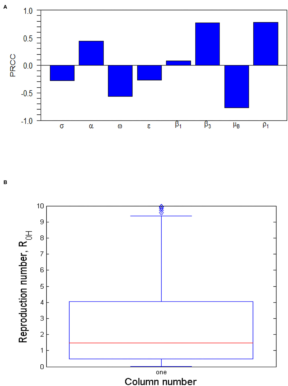
Figure 4. (A) Tornado plot of Partial Rank Correlation Coefficient (PRCC) values for some important parameters of ${{R}}_{0H}$. The parameter values (ranges) used are given in Table 2. (B) Box plot of ${{R}}_{0H}$. The parameter values (ranges) used are given in Table 2.

TABLE 3

Table 3. Parameter partial rank correlation coefficient (PRCC) significance (unadjusted p-values).

Furthermore, the Monte Carlo simulations of the most sensitivity parameters are displayed as scatter plots in Figure 5. They show how the most sensitivity parameters are affecting ${{R}}_{0H}$ positively or negatively. From Figure 5, the parameters, β₃, ω, μ_B, and ρ₁, have a strong force to reckon with in the transmission dynamics of the MPXV infection and should be targeted by public health practitioners and decision-makers in order to curtail the MPX infection in the population.

FIGURE 5

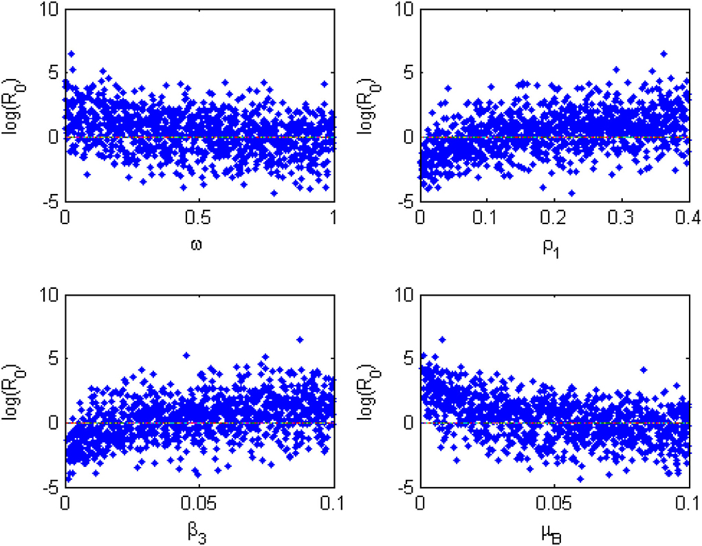
Figure 5. Monte Carlo simulations for the most sensitive parameters of the model generated using the parameter values in Table 2.

The pairwise PRCC comparison of some model parameters whose p-values are less than 0.05 is presented in Tables 4, 5. The pairwise PRCC comparison is carried out to determine which of the compared parameter processes are different. Table 4 is for unadjusted p-values while Table 5 is for false discovery rate (FDR) adjusted p-values. In Tables 4, 5, the compared pair of significant parameters that are less than 0.05 means that they are significantly different (TRUE) otherwise they are not different (FALSE). We notice that the pairs σ − ϵ and β₃ − ρ₁ are not significantly different in both Tables 4, 5. This is further shown in Table 6 that all the most sensitive compared pairs are significantly different, except the pairs σ − ϵ and β₃ − ρ₁. The pair β₃ − ρ₁ is related as they contribute to the environmental transmission that aggravates the spread of MPX infection. Meanwhile, the pair σ − ϵ is not related as σ is the quarantine rate and ϵ is the vaccination rate but their processes are significant to halt the spread of MPX infection. The impacts of insignificant pairs (σ − ϵ and β₃ − ρ₁) on ${{R}}_{0H}$ are displayed in Figures 6A,C.

TABLE 4

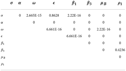
Table 4. Pairwise PRCC comparison (unadjusted P-values).

TABLE 5

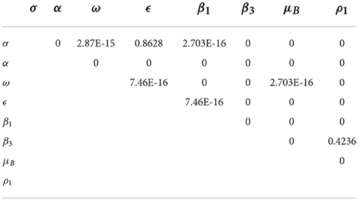
Table 5. Pairwise PRCC comparisons (FDR adjusted P-values).

TABLE 6

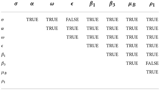
Table 6. Parameters different after FDR adjustment.

FIGURE 6

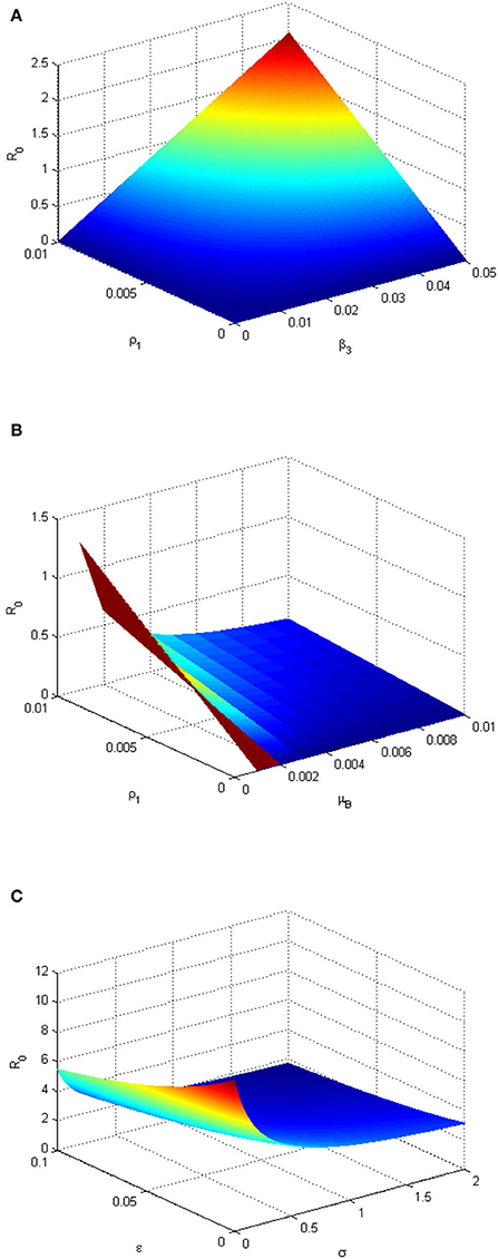
Figure 6. (A) Three-dimensional plot depicting the relationship between ${{R}}_{0H}$ and environmental transmission rate (β₃), infected human shedding rate (ρ₁), and ${{R}}_{0H}$. The plot shows the sensitivity of the ${{R}}_{0H}$ to the changes (variation) of the parameters β₃ and ρ₁. (B) Three-dimensional plot depicting the relationship between the decay rate of MPXV in the environment (μ_B), ρ₁ and ${{R}}_{0H}$. The graph shows the sensitivity of the ${{R}}_{0H}$ to the changes (variation) of the parameters μ_B and ρ. (C) Three-dimensional plot depicting the relationship between quarantine rate (σ), ϵ, and ${{R}}_{0H}$. The graph shows the sensitivity of the ${{R}}_{0H}$ to the changes (variation) of the parameters σ and ϵ. The parameter values used are given in Table 2.

Figure 6A depicts that the value of ${{R}}_{0H}$ increases as the environmental transmission rate (β₃) and infectious human shedding rate (ρ₁) increase and when they are close to 0, when ${{R}}_{0H}<1$, it means there is a high degree of sensitivity of these parameters to ${{R}}_{0H}$. This implies that the MPXV infection can be eliminated in the population if susceptible humans avoid contact with MPX-contaminated environment while the infected humans stop shedding the infection within the environment. In the absence (or very low level) of ρ₁, ${{R}}_{0H}<1$ provided that the decay rate of the contaminated environment (μ_B) keeps increasing (Figure 6B). This implies that the more the monkeypox-contaminated environment is cleaned and the shedding rate of infectious individuals in the environment is reduced (keeping at a very low level), the more the monkeypox infection will be eradicated within the population. Figure 6C shows that increasing the vaccination and quarantine rates (ϵandσ) reduces the value of ${{R}}_{0H}$. Thus, this implies that the MPXV infection will be curtailed within the human population if more susceptible humans are vaccinated and exposed humans are quarantined.

6. Numerical simulations

Numerical simulations for the model system (1–9) are performed using MATLAB ODE45 solver and the parameter values used are in Table 2, except where they are stated otherwise. The simulations illustrate and support the analytical results already established in Section 4. The following initial conditions, S_H(0) = 8000, V_H(0) = 5000, E_H(0) = 300, Q_H(0) = 100, I_H(0) = 50, R_H(0) = 0, S_R(0) = 3000, I_R(0) = 100, and B(0) = 50 are used for the simulations. Figure 7 demonstrates the impacts of the most sensitive parameters. This is based on the result of sensitivity analysis. Figure 7A illustrates the effect of the decay rate of MPXV in the environment, μ_B, on the infected human population. From Figure 7A, as the value of μ_B increases from 0.003 to 1, ${{R}}_{0H}$ reduces from 1.6487(forμ_B = 0.003) to 0.005(forμ_B = 1.0), respectively. This indicates that increasing the decay rate of MPXV in the environment will drastically reduce the number of infected humans in the population and this supports the scatter plot in Figure 5. From Figure 7B, we observe that the more infected humans shed the infection in the environment, the more people get infected and this may lead to an endemic situation of MPXV in the population. The dynamics of the infected human population when varying environmental transmission rate (β₃), is shown in Figure 7C. We noticed that as β₃ increases from 0.001 to 0.5, it increases the value of ${{R}}_{0H}$ from 0.1649 to 82.4364, which leads to an increase in the number of infected humans in the population. In particular, when β₃ is 0.001 (or close to zero), ${{R}}_{0H}<1$, and this consequently results in the elimination of the MPXV infection in the population after the first 150 days. This reveals that susceptible humans contract the MPXV disease more when they have frequent contact with MPXV contaminated environment. On the other hand, Figure 7D presents the effect of quarantining the exposed humans in the population. We observe that as the quarantine rate (σ) is increasing from 0.02 to 2.0, it reduces value of ${{R}}_{0H}$ from 5.1072 to 1.6487. It initially drops the number of infected humans to below 50 before shooting up after 10 days and reduces again after 45 days which leads to the persistence and spread of MPXV in the human population as ${{R}}_{0H}>1$. This reveals that quarantine intervention alone cannot halt the spread of MPXV within the population but it can be complemented with other interventions to achieve complete eradication of MPXV in the population.

FIGURE 7

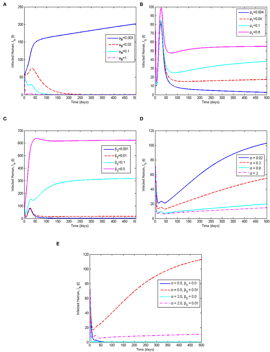
Figure 7. Simulation results showing (A) the effect of μ_B on the infected human population, (B) the effect of ρ₁ on the infected human population, (C) the effect of β₃ on the infected human population, (D) the effect of quarantine rate (σ) on the infected human population, and (E) the combined effect of σ and the environmental transmission rate β₃ on the infected human population. The parameter values used are given in Table 2.

This study is in agreement and consistent with the results of Somma et al. [8] and Emeka et al. [14] that quarantine (isolation) can only reduce the MPXV disease transmission but does not eliminate the infection within the population. Furthermore, the combined effect of quarantine rate (σ) and environmental transmission rate (β₃) is considered in Figure 7E. It shows that in the absence of the environmental transmission rate (β₃ = 0) for any quarantine rate (σ = 0, orσ = 2.0), the number of infected humans reduces rapidly to 0 after 100 days leading to a monkeypox-free population. Whereas, whenever there is environment transmission rate (β₃ = 0.01) for any rate of quarantine, (σ = 0, orσ = 2.0), the number of infected humans increases in the population which is more in the absence of quarantine intervention (σ = 0). The implication of Figure 7E is that a MPX-free population can be achieved if there is no contact with MPX contaminated environment.

7. Conclusion

An epidemiological model for the transmission dynamics of the MPX disease is formulated and rigorously analyzed for human and rodent populations. Using the next-generation approach, we computed ${{R}}_0$ that results in two R₀ for the two host populations, namely ${{R}}_{0R}$ and ${{R}}_{0H}$. The local and global stabilities of the MPXV-FE are established in terms of ${{R}}_{0H}$. The formulated model exhibits three equilibria, namely MPXV-FE, IRF-EE, and CO-EE. The global stability of the IRF-EE is proved using the Volterra-Lyapunov matrix theory. Furthermore, sensitivity analysis of $({{R}}_{0H})$ is performed using the LHS/PRCC techniques to examine the model parameters with the greatest impact on ${{R}}_{0H}$. The results from the sensitivity analysis indicated that the environmental parameters (environmental transmission rate, decay rate of MPXV in the environment, and infected humans shedding rate) played an important role in the spread of the MPX disease among host populations. This is further supported by numerical simulations and the results revealed that quarantine intervention should be complemented by other interventions to curtail the spread of the MPX disease in the population. It also suggests that health care practitioners and policy-makers should focus more on how to increase the environmental decay rate of the monkeypox virus, as well as, reduce the environmental transmission rate and the shedding rate of infectious individuals into the environment. Since it is very difficult to control the rodent population, we observed from our study that the best way to prevent, mitigate, and control the MPX disease is to avoid contact with infected humans and the monkeypox contaminated environment. This is done through educating the human population about the disease, observing personal hygiene, sterilization of medical equipment, and wearing personal protective equipment (PPE) when treating an infected human and promoting vaccination against the MPX infection in highly endemic areas of the MPX infection as an additional intervention measure.

There are some limitations to our studies. One of them is using real-life data to estimate the parameters of the model rather than sourcing the parameter values from existing literature on the dynamics of the MPX disease. Second, the climate change effect is not considered in this study even though it possibly affects the rodent population.

The formulated model may be extended by incorporating the interaction between susceptible rodents and the environment using half saturation function and a logistic growth function of the pathogens in the environment. It may also subdivide the infected humans into mildly infected humans, symptomatically infected humans, and isolated humans. The optimal control analysis of the formulated model in the presence of different intervention strategies may be considered for future work.

Data availability statement

The original contributions presented in the study are included in the article/supplementary material, further inquiries can be directed to the corresponding author.

Author contributions

CM, IO, and GN contributed to conception and model formulation of the study. CM, IO, GN, and ZC contributed to the analysis and write-up of sections of the manuscript. All authors contributed to manuscript revision, read, and approved the final version of the manuscript.

Acknowledgments

The authors would like to thank their respective universities for their support toward this manuscript.

Conflict of interest

The authors declare that the research was conducted in the absence of any commercial or financial relationships that could be construed as a potential conflict of interest.

Publisher's note

All claims expressed in this article are solely those of the authors and do not necessarily represent those of their affiliated organizations, or those of the publisher, the editors and the reviewers. Any product that may be evaluated in this article, or claim that may be made by its manufacturer, is not guaranteed or endorsed by the publisher.

References

1. WHO. Monkeypox. WHO (2022). Available from: Available online at: https://www.who.int/en/news-room/fact-sheets/detail/monkeypox

2. Jezek Z, Szczeniowski M, Paluku K, Mutombo M, Grab B. Human monkeypox: confusion with chickenpox. Acta Trop. (1988) 45:297–307.

PubMed Abstract | Google Scholar

3. CDC2. Monkeypox Q & A: What You Need to Know About Monkeypox. CDC (2022). Available from: Available online at: https://www.who.int/europe/news/item/10-06-2022-monkeypox-q-a–what-you-need-to-know-about-monkeypox

4. CDC. Monkeypox Signs and Symptoms. CDC (2022). Available from: Available online at: https://www.cdc.gov/poxvirus/monkeypox/

5. Nolen LD, Osadebe L, Katomba J, Likofata J, Mukadi D, Monroe B, et al. Extended human-to-human transmission during a monkeypox outbreak in the Democratic Republic of the Congo. Emerg Infect Dis. (2016) 22:1014–21. doi: 10.3201/eid2206.150579

PubMed Abstract | CrossRef Full Text | Google Scholar

6. NCDC. Update on Monkeypox (MPX) in Nigeria, Epi-week: 23, June 12 2022. NCDC (2022). Available from: Available online at: https://ncdc.gov.ng/diseases/sitreps/?cat=8&name=An%20Update%20of%20Monkeypox%20Outbreak%20in%20Nigeria

7. Alakunle E, Moens U, Nchinda G, Okeke MI. Monkeypox virus in Nigeria: infection biology, epidemiology, and evolution. Viruses. (2020) 12:1257. doi: 10.3390/v12111257

PubMed Abstract | CrossRef Full Text | Google Scholar

8. Somma SA, Akinwande NI, Chado UD. A mathematical model of monkey pox virus transmission dynamics. Ife J Sci. (2019) 21:195–204. doi: 10.4314/ijs.v21i1.17

CrossRef Full Text | Google Scholar

9. Fowotade A, Fasuyi TO, Bakare RA. Re-emergence of monkeypox in Nigeria: a cause for concern and public enlightenment. Afr J Clin Exp Microbiol. (2018) 19:307–13. doi: 10.4314/ajcem.v19i4.9

CrossRef Full Text | Google Scholar

10. Madubueze CE, Dachollom S, Onwubuya IO. Controlling the spread of COVID-19: optimal control analysis. Comput Math Methods Med. (2020) 2020:6862516. doi: 10.1101/2020.06.08.20125393

PubMed Abstract | CrossRef Full Text | Google Scholar

11. Ogunmiloro OM. Modeling the dynamics of the consequences of demographic disparities in the transmission of Lassa fever disease in Nigeria. Earth Syst Environ. (2022) doi: 10.1007/s40808-022-01522-3. [Epub ahead of print].

CrossRef Full Text | Google Scholar

12. Lasisi NO, Akinwande NI, Oguntolu FA. Development and exploration of a mathematical model for transmission of monkey-pox disease in humans. Math Models Eng. (2020) 6:23–33. doi: 10.21595/mme.2019.21234

CrossRef Full Text | Google Scholar

13. Usman S, Adamu II. Modeling the transmission dynamics of the monkeypox virus infection with treatment and vaccination interventions. J Appl Math Phys. (2017) 5:2335–53. doi: 10.4236/jamp.2017.512191

CrossRef Full Text | Google Scholar

14. Emeka PC, Ounorah MO, Eguda FY, Babangida BG. Mathematical model for monkeypox virus transmission dynamics. Epidemiology (Sunnyvale). (2018) 8:348. doi: 10.4172/2161-1165.1000348

CrossRef Full Text

15. Peter OJ, Kumar S, Kumari N, Oguntolu FA, Oshinubi K, Musa R. Transmission dynamics of Monkeypox virus: a mathematical modelling approach. Model Earth Syst Environ. (2022) 8:3423–34. doi: 10.1007/s40808-021-01313-2

PubMed Abstract | CrossRef Full Text | Google Scholar

16. Keeling MJ, Rohani P. Controlling infectious diseases. In: Modeling Infectious Diseases in Humans and Animals. Princeton, NJ: Princeton University Press (2011). p. 291–336.

Google Scholar

17. Ogunmiloro OM. Mathematical analysis and approximate solution of a fractional order caputo fascioliasis disease model. Chaos Solit Fractals. (2021) 146:110851. doi: 10.1016/j.chaos.2021.110851

CrossRef Full Text | Google Scholar

18. Martcheva M. An Introduction to Mathematical Epidemiology. Vol. 61. New York, NY: Springer (2015).

Google Scholar

19. Marennikova S, Šeluhina E. Susceptibility of some rodent species to monkeypox virus, and course of the infection. Bull World Health Organ. (1976) 53:13–20.

PubMed Abstract | Google Scholar

20. Ježek Z, Szczeniowski M, Paluku K, Mutombo M. Human monkeypox: clinical features of 282 patients. J Infect Dis. (1987) 156:293–8. doi: 10.1093/infdis/156.2.293

PubMed Abstract | CrossRef Full Text | Google Scholar

21. Hethcote HW. The mathematics of infectious diseases. SIAM Rev. (2000) 42:599–653. doi: 10.1137/S0036144500371907

CrossRef Full Text | Google Scholar

22. Berge T, Chapwanya M, Lubuma JS, Terefe Y. A mathematical model for Ebola epidemic with self-protection measures. J Biol Syst. (2018) 26:107–31. doi: 10.1142/S0218339018500067

CrossRef Full Text | Google Scholar

23. Tian JP, Wang J. Global stability for cholera epidemic models. Math Biosci. (2011) 232:31–41. doi: 10.1016/j.mbs.2011.04.001

PubMed Abstract | CrossRef Full Text | Google Scholar

24. Busenberg S, Cooke K. Vertically Transmitted Diseases: Models and Dynamics. Vol. 23. Heidelberg: Springer Berlin, Heidelberg (2012).

Google Scholar

25. Stuart A, Humphries AR. Dynamical Systems and Numerical Analysis. England: Cambridge University Press (1998).

Google Scholar

26. Diekmann O, Heesterbeek J, Roberts MG. The construction of next-generation matrices for compartmental epidemic models. J R Soc Interface. (2010) 7:873–85. doi: 10.1098/rsif.2009.0386

PubMed Abstract | CrossRef Full Text | Google Scholar

27. Kim JH, Su W, Song YJ. On stability of a polynomial. J Appl Math Inf. (2018) 36:231–36. doi: 10.14317/jami.2018.231

CrossRef Full Text | Google Scholar

28. Heffernan JM, Smith RJ, Wahl LM. Perspectives on the basic reproductive ratio. J R Soc Interface. (2005) 2:281–93. doi: 10.1098/rsif.2005.0042

PubMed Abstract | CrossRef Full Text | Google Scholar

29. Bassey BE, Atsu JU. Global stability analysis of the role of multi-therapies and non-pharmaceutical treatment protocols for COVID-19 pandemic. Chaos Solit Fractals. (2021) 143:110574. doi: 10.1016/j.chaos.2020.110574

PubMed Abstract | CrossRef Full Text | Google Scholar

30. Chien F, Shateyi S. Volterra-Lyapunov stability analysis of the solutions of babesiosis disease model. Symmetry. (2021) 13:1272. doi: 10.3390/sym13071272

CrossRef Full Text | Google Scholar

31. Castillo-Chavez C, Blower S, Van den Driessche P, Kirschner D, Yakubu AA. Mathematical Approaches for Emerging and Reemerging Infectious Diseases: Models, Methods, and Theory. New York, NY: Springer (2002).

Google Scholar

32. Zahedi MS, Kargar NS. The Volterra-Lyapunov matrix theory for global stability analysis of a model of the HIV/AIDS. Int J Biomath. (2017) 10:1750002. doi: 10.1142/S1793524517500024

CrossRef Full Text | Google Scholar

33. Blower SM, Dowlatabadi H. Sensitivity and uncertainty analysis of complex models of disease transmission: an HIV model, as an example. Int Stat Rev. (1994) 62:229–43. doi: 10.2307/1403510

CrossRef Full Text | Google Scholar

34. Rodrigues HS, Monteiro MTT, Torres DF. Sensitivity analysis in a dengue epidemiological model. Conf Papers Math. (2013) 2013:721406. doi: 10.1155/2013/721406

CrossRef Full Text | Google Scholar

35. Madubueze CE, Chazuka Z, Onwubuya I, Chukwu W, Chukwu C. On the mathematical modelling of Schistosomiasis transmission dynamics with heterogeneous intermediate host. Front Appl Math Stat. (2022) 8:1020161. doi: 10.3389/fams.2022.1020161

PubMed Abstract | CrossRef Full Text | Google Scholar

36. Chukwu C, Juga M, Chazuka Z, Mushanyu J. Mathematical analysis and sensitivity assessment of HIV/AIDS-Listeriosis co-infection dynamics. Int J Appl Comput Math. (2022) 8:1–21. doi: 10.1007/s40819-022-01458-3

PubMed Abstract | CrossRef Full Text | Google Scholar

37. Chazuka Z, Moremedi G, Rapoo E. In-Host Dynamics of the Human Papillomavirus (HPV) in the Presence of Immune Response. In: International Symposium on Mathematical and Computational Biology. Cham: Springer (2020). p. 79–97.

Google Scholar

38. Njagarah JB, Nyabadza F, Kgosimore M, Hui C. Significance of antiviral therapy and CTL-mediated immune response in containing hepatitis B and C virus infection. Appl Math Comput. (2021) 397:125926. doi: 10.1016/j.amc.2020.125926

CrossRef Full Text | Google Scholar

39. Di Giulio DB, Eckburg PB. Human monkeypox: an emerging zoonosis. Lancet Infect Dis. (2004) 4:15–25. doi: 10.1016/S1473-3099(03)00856-9

PubMed Abstract | CrossRef Full Text | Google Scholar

40. Bhunu C, Garira W, Magombedze G. Mathematical analysis of a two strain HIV/AIDS model with antiretroviral treatment. Acta Biotheor. (2009) 57:361–81. doi: 10.1007/s10441-009-9080-2

PubMed Abstract | CrossRef Full Text | Google Scholar

41. Bhunu C, Mushayabasa S. Modelling the transmission dynamics of pox-like infections. IAENG Int J Appl Math. (2011) 41:141–9.

Google Scholar

42. Odom MR, Hendrickson RC, Lefkowitz EJ. Poxvirus protein evolution: family wide assessment of possible horizontal gene transfer events. Virus Res. (2009) 144:233–49. doi: 10.1016/j.virusres.2009.05.006

PubMed Abstract | CrossRef Full Text | Google Scholar