Bifurcation analysis of a predator–prey model involving age structure, intraspecific competition, Michaelis–Menten type harvesting, and memory effect

1. Introduction

Since Lotka and Volterra introduced the classical predator–prey model, theoretical studies of predation without age structure have attracted the attention of many authors, for example Deng et al. [1], Huang et al. [2], Tahara et al. [3], and Zeng et al. [4]. However, in nature, many species of plants and animals could have life histories that can simply be partitioned into two age stages: immature and mature stages. In each stage, individuals of species have identical biological characteristics, such as the ability to reproduce, motile, ingest food, and survive [5]. In particular, there are amphibians, insects, birds, and mammals with life cycles that can last from only several days or weeks to more than a century. For this reason, some researchers have developed the predator–prey model by incorporating age structure either in prey or/and predator population with other factors that also influence the dynamics of the predator–prey model, mainly restricted to the classical integer-order, stochastic, or delay equations [6–13].

In Wang and Chen [14] considered the predator–prey model with age structure for the predator population using time delays. If we ignore the effect of time delay, the model can be written as follows:

$\begin{array}{ll}\begin{array}{l}\frac{dx}{dt}=rx\left(1-\frac{x}{K}\right)-mxz,\\ \frac{dy}{dt}=nxz-\beta y-{\delta }_{1}y,\\ \frac{dz}{dt}=\beta y-{\delta }_{2}z.\end{array}& (1)\end{array}$

Here x(t), y(t), and z(t) represent the population densities of prey, immature predator, and mature predator, at time t, respectively. Model (Equation 1) assumes that the prey grows logistically with r as the intrinsic growth rate, K is the carrying capacity; m is the linear Holling type I functional response, n is the conversion rate with which captured prey are converted to new immature predator, β is the maturity rate of the predator, δ₁ and δ₂ are the death rate of the immature and mature predators, respectively. It is also assumed that only the mature predator can feed the prey through the term mxz. If we do not consider the age structure of the predator population, then model (Equation 1) is reduced to the classical Lotka–Volterra model for which the positive equilibrium or the boundary equilibrium of this model is globally asymptotically stable. This means that the model has no periodic solution. On the other hand, Wang and Chen [14] prove that in the model (Equation 1), there exists an orbitally asymptotically stable periodic solution around the interior equilibrium point which suggests that the age structure can cause periodic oscillation of populations.

From the point of view of human needs, harvesting of populations generally occurs in wildlife, forestry, and fisheries management. When harvesting is integrated into the predator–prey model, there are three types of harvesting, namely constant harvesting [15], linear harvesting [16], and non-linear harvesting [17]. In this article, we assume that the predator is not a commercial species and there is intraspecific competition among immature predators. Therefore, the predator–prey model with age structure and intraspecific competition in predator (Equation 1), where the prey population is subject to Michaelis–Menten type harvesting, is given by

$\begin{array}{ll}\begin{array}{l}\frac{dx}{dt}=rx\left(1-\frac{x}{K}\right)-mxz-\frac{hx}{c+x},\\ \frac{dy}{dt}=nxz-\beta y-{\delta }_{1}y-\omega y^2,\\ \frac{dz}{dt}=\beta y-{\delta }_{2}z.\end{array}& (2)\end{array}$

An example of prey-predator interactions whose biological phenomena are described in the model (Equation 2) can be found in the African wild dog with its prey impala. The African wild dogs are a social structure that lives in packs. For 3–4 weeks, young African wild dogs were in the den with their mother. All adult members of African wild dogs are care for their young ones and provide food for them. The hunting members of the pack will return to the den where they regurgitate meat for the nursing female and young. In some cases, young ones fail to survive because the hunting member does not bring back sufficient food for the young, which leads to intraspecific competition in immature predator [18]. On the other hand, the prey, impala, even though there are no major threats to their survival, poaching has become significantly contributed to the decline in its number [19].

Note that the growth rates of the prey, immature, and mature predator populations in the model (Equation 2) depend only on the local state as the left-hand side is the integer-order derivative. On the other hand, most biological systems have properties where the current state is affected by all of the past states or it is called the memory effect. Therefore, modeling with memory effects can be done by analyzing the system using fractional-order calculus [20, 21]. The operators of the fractional-order derivative have non-local properties to make them more suitable for dynamical systems that have memory influences on their state variables.

After Riemann and Liouville generalized the concept of integer-order calculus to the fractional-order calculus over two decades ago, the studies about the predator–prey models with fractional-order differential equation have gained much attention, for example, Rahmi et al. [22], Owolabi [23], Barman et al. [24], Ghanbari and Djilali [25], Yousef et al. [26], Ghosh et al. [27], and Panigoro et al. [28]. The fractional-order derivatives are defined as an integration that provides the ability to store the whole memory over time, and hence, it could give an exact description of different ecological phenomena. For this reason, the new structure for the model (Equation 2) is given in the following form:

$\begin{array}{ll}\begin{array}{l}{}^C{{D}}_t^{\alpha }x(t)=rx\left(1-\frac{x}{K}\right)-mxz-\frac{hx}{c+x}=F_1(x,y,z),\\ {}^C{{D}}_t^{\alpha }y(t)=nxz-\beta y-{\delta }_{1}y-\omega y^2=F_2(x,y,z),\\ {}^C{{D}}_t^{\alpha }z(t)=\beta y-{\delta }_{2}z=F_3(x,y,z).\end{array}& (3)\end{array}$

The existence and local stability of all equilibrium points of the model (Equation 3) are discussed in Panigoro et al. [29]. However, to the best of our knowledge, the global dynamics and bifurcation analysis of the model (Equation 3), to this day, have not been investigated. Here, ${}^C{{D}}_t^{\alpha }f(t)$ is the standard Caputo derivative for a continuous function f(x) ∈ ℂ([0, +∞), ℝ), which is defined as follows:

$\begin{array}{ll}{}^C{{D}}_t^{\alpha }f(t)=\frac{1}{\Gamma (1-\alpha )}{\displaystyle {\int }_0^t}\frac{f^{\prime }(\tau )}{{(t-\tau )}^{\alpha }}d\tau ,& (4)\end{array}$

where Γ(∗) is the gamma function, t ≥ 0, and 0 < α ≤ 1 is known as the order of the fractional derivative.

Based on the above discussion, we have organized our work in several sections: In Section 3, we develop the existence and uniqueness solution of the model (Equation 3). To check the biologically well-posedness of the model, we establish the non-negativity and boundedness of solutions of the model in Section 3. In Section 4, we derive some sufficient conditions to ensure the global asymptotic stability of each locally asymptotically stable equilibrium point by applying the Lyapunov functions. We then analyze the existing conditions of transcritical, saddle-node, backward, and Hopf bifurcations in Section 5. Some numerical simulations of our obtained results are carried out in Section 6. Finally, the conclusions are given in Section 7.

2. Existence and uniqueness

In this section, we will show that the model (Equation 3) has a unique solution. A similar manner given by Mahata et al. [30] is adopted. We first take the Riemann–Liouville integral (Definition 1 in Yavuz and Sene [31]) on both sides of Equation (3) to achieve the following Volterra-type integral equations.

$\begin{array}{l}x(t)-x(0)=\frac{1}{\Gamma (\alpha )}{\displaystyle {\int }_0^t}{F}_1(x(\tau ),y(\tau ),z(\tau )){(t-)}^{\alpha -1}d\tau ,\\ y(t)-y(0)=\frac{1}{\Gamma (\alpha )}{\displaystyle {\int }_0^t}{F}_2(x(\tau ),y(\tau ),z(\tau )){(t-\tau )}^{\alpha -1}d\tau ,\\ z(t)-z(0)=\frac{1}{\Gamma (\alpha )}{\displaystyle {\int }_0^t}{F}_3(x(\tau ),y(\tau ),z(\tau )){(t-\tau )}^{\alpha -1}d\tau ,& (5)\end{array}$

Now, we will show that the kernels F_i(x, y, z), i = 1, 2, 3, satisfy the Lipschitz condition. For ∥.∥ is the Euclidean norm, we suppose that ∥x(t)∥ ≤ a₁, $\parallel \bar{x}(t)\parallel \le a_2$, ∥y(t)∥ ≤ a₃, ∥$\bar{y}$(t)∥ ≤ a₄, ∥z(t)∥ ≤ a₅, and $\parallel \bar{z}(t)\parallel \le a_6$ are bounded functions. For x, $\bar{x}$, y, $\bar{y}$, z, and $\bar{z}$, we have

$\begin{array}{l}\parallel F_1(x,y,z)-F_1(\bar{x},y,z)\parallel \\ =\left|\right|\left[rx\left(1-\frac{x}{K}\right)-mxz-\frac{hx}{c+x}\right]\\ -\left[r\bar{x}\left(1-\frac{\bar{x}}{K}\right)-m\bar{x}z-\frac{h\bar{x}}{c+\bar{x}}\right]\left|\right|\\ =\left|\right|r(x-\bar{x})-\frac{r}{K}(x+\bar{x})(x-\bar{x})-mz(x-\bar{x})\\ -ch\left(\frac{x-\bar{x}}{(c+x)(c+\bar{x})}\right)\left|\right|\\ \le r\parallel x-\bar{x}\parallel +\frac{(a_1+a_2)r}{K}\parallel x-\bar{x}\parallel +a_{5}m\parallel x-\bar{x}\parallel +\frac{h}{c}\parallel x-\bar{x}\parallel \\ =g_1\parallel x-\bar{x}\parallel ,\\ \parallel F_2(x,y,z)-F_2(x,\bar{y},z)\parallel \\ =\parallel \left[nxz-\beta y-{\delta }_{1}y-\omega y^2\right]-\left[nxz-\beta \bar{y}-{\delta }_1\bar{y}-\omega {\bar{y}}^2\right]\parallel \\ =\parallel -\beta (y-\bar{y})-{\delta }_1(y-\bar{y})-\omega (y+\bar{y})(y-\bar{y})\parallel \\ \le \beta \parallel y-\bar{y}\parallel +{\delta }_1\parallel y-\bar{y}\parallel +\omega (a_3+a_4)\parallel y-\bar{y}\parallel \\ =g_2\parallel y-\bar{y}\parallel ,\\ \parallel F_3(x,y,z)-F_3(x,y,\bar{z})\parallel \\ =\parallel \left[\beta y-{\delta }_{2}z\right]-\left[\beta y-{\delta }_2\bar{z}\right]\parallel \\ \le g_3\parallel z-\bar{z}\parallel ,\end{array}$

where $g_1=r+\frac{(a_1+a_2)r}{K}+a_{5}m+\frac{h}{c}$, g₂ = β + δ₁ + ω(a₃ + a₄), and g₃ = δ₂. Therefore, we conclude that F_i(x, y, z), i = 1, 2, 3, satisfy the Lipschitz condition. Furthermore, it is clear that if 0 ≤ g_i < 1, then F_i(x, y, z) are contractions for i = 1, 2, 3. Therefore, the following theorem is obtained.

Theorem 1. The kernel F_i(x, y, z), i = 1, 2, 3 satisfy the Lipschitz condition and contractions if 0 < g_i < 1, i = 1, 2, 3.

Next, Equation (5) can be written as follows:

$\begin{array}{l}x(t)=x(0)+\frac{1}{\Gamma (\alpha )}{\displaystyle {\int }_0^t}{F}_1(x(\tau ),y(\tau ),z(\tau )){(t-\tau )}^{\alpha -1}d\tau ,\\ y(t)=y(0)+\frac{1}{\Gamma (\alpha )}{\displaystyle {\int }_0^t}{F}_2(x(\tau ),y(\tau ),z(\tau )){(t-\tau )}^{\alpha -1}d\tau ,\\ z(t)=z(0)+\frac{1}{\Gamma (\alpha )}{\displaystyle {\int }_0^t}{F}_3(x(\tau ),y(\tau ),z(\tau )){(t-\tau )}^{\alpha -1}d\tau ,\end{array}$

Which can be written by the following recursive formula

$\begin{array}{l}{x}_n(t)=x(0)+\frac{1}{\Gamma (\alpha )}{\displaystyle {\int }_0^t}{F}_1(x_{n-1},y,z){(t-\tau )}^{\alpha -1}d\tau ,\\ y_n(t)=y(0)+\frac{1}{\Gamma (\alpha )}{\displaystyle {\int }_0^t}{F}_2(x,y_{n-1},z){(t-\tau )}^{\alpha -1}d\tau ,\\ z_n(t)=z(0)+\frac{1}{\Gamma (\alpha )}{\displaystyle {\int }_0^t}{F}_3(x,y,z_{n-1}){(t-\tau )}^{\alpha -1}d\tau ,\end{array}$

with initial conditions x₀(t) = x(0), y₀(t) = y(0), and z₀(t) = z(0). Therefore, we have

$\begin{array}{l}{\phi }_{1_n}(t)=x_n(t)-x_{n-1}(t)\\ =\frac{1}{\Gamma (\alpha )}{\displaystyle {\int }_0^t}(F_1(x_{n-1},y,z)-F_1(x_{n-2},y,z)){(t-\tau )}^{\alpha -1}d\tau ,\\ {\phi }_{2_n}(t)=y_n(t)-y_{n-1}(t)\\ =\frac{1}{\Gamma (\alpha )}{\displaystyle {\int }_0^t}(F_2(x,y_{n-1},z)-F_2(x,y_{n-2},z)){(t-\tau )}^{\alpha -1}d\tau ,\\ {\phi }_{3_n}(t)=z_n(t)-z_{n-1}(t)\\ =\frac{1}{\Gamma (\alpha )}{\displaystyle {\int }_0^t}(F_3(x,y,z_{n-1})-F_3(x,y,z_{n-2})){(t-\tau )}^{\alpha -1}d\tau ,& (6)\end{array}$

where $x_n(t)=\sum _{j=1}^n{\phi }_{1_n}(t)$, $y_n(t)=\sum _{j=1}^n{\phi }_{2_n}(t)$, and $z_n(t)=\sum _{j=1}^n{\phi }_{3_n}(t)$. Now, we evaluate the norm of Equation (6). We achieve

$\begin{array}{l}\parallel {\phi }_{1_n}(t)\parallel =\parallel x_n(t)-x_{n-1}(t)\parallel \\ \le \frac{1}{\Gamma (\alpha )}{\displaystyle {\int }_0^t}\left|\right|(F_1(x_{n-1},y,z)\\ -F_1(x_{n-2},y,z)){(t-\tau )}^{\alpha -1}d\tau ,\\ \parallel {\phi }_{2_n}(t)\parallel =\parallel y_n(t)-y_{n-1}(t)\parallel \\ \le \frac{1}{\Gamma (\alpha )}{\displaystyle {\int }_0^t}\left|\right|(F_2(x,y_{n-1},z)\\ -F_2(x,y_{n-2},z)){(t-\tau )}^{\alpha -1}d\tau \left|\right|,\\ \parallel {\phi }_{3_n}(t)\parallel =\parallel z_n(t)-z_{n-1}(t)\parallel \\ \le \frac{1}{\Gamma (\alpha )}{\displaystyle {\int }_0^t}\left|\right|(F_3(x,y,z_{n-1})\\ -F_3(x,y,z_{n-2})){(t-\tau )}^{\alpha -1}d\tau \left|\right|.& (7)\end{array}$

From Theorem 1, we have that the kernel satisfy the Lipschitz condition and hence Equation (7) becomes

$\begin{array}{l}\parallel x_n(t)-x_{n-1}(t)\parallel \le \frac{g_1}{\Gamma (\alpha )}{\displaystyle {\int }_0^t}\parallel x_{n-1}-x_{n-2}\parallel {(t-\tau )}^{\alpha -1}d\tau ,\\ \parallel y_n(t)-y_{n-1}(t)\parallel \le \frac{g_2}{\Gamma (\alpha )}{\displaystyle {\int }_0^t}\parallel y_{n-1}-y_{n-2}\parallel {(t-\tau )}^{\alpha -1}d\tau ,\\ \parallel z_n(t)-z_{n-1}(t)\parallel \le \frac{g_3}{\Gamma (\alpha )}{\displaystyle {\int }_0^t}\parallel z_{n-1}-z_{n-2}\parallel {(t-\tau )}^{\alpha -1}d\tau .\end{array}$

The last inequality gives

$\begin{array}{l}\parallel {\phi }_{1_n}(t)\parallel \le \frac{g_1}{\Gamma (\alpha )}{\displaystyle {\int }_0^t}\parallel {\phi }_{1_{n-1}}(\tau )\parallel d\tau ,\\ \parallel {\phi }_{2_n}(t)\parallel \le \frac{g_2}{\Gamma (\alpha )}{\displaystyle {\int }_0^t}\parallel {\phi }_{2_{n-1}}(\tau )\parallel d\tau ,\\ \parallel {\phi }_{3_n}(t)\parallel \le \frac{g_3}{\Gamma (\alpha )}{\displaystyle {\int }_0^t}\parallel {\phi }_{3_{n-1}}(\tau )\parallel d\tau .& (8)\end{array}$

Finally, the existence of a solution is given by the following theorem.

Theorem 2. The solution of model (Equation 3) has a solution under the condition if we have t₁ such that $\left(\frac{t_1{g}_i}{\Gamma (\alpha +1)}\right)<1,i=1,2,3$.

Proof. We assume that x(t), y(t), and z(t) are bounded and their kernel F_i, i = 1, 2, 3 satisfy the Lipschitz condition. According to Equation (8), we obtain

$\begin{array}{l}\parallel {\phi }_{1_n}(t)\parallel \le \parallel x_0(t)\parallel {\left[\frac{t_1{g}_1}{\Gamma (\alpha +1)}\right]}^n,\\ \parallel {\phi }_{2_n}(t)\parallel \le \parallel y_0(t)\parallel {\left[\frac{t_1{g}_2}{\Gamma (\alpha +1)}\right]}^n,\\ \parallel {\phi }_{3_n}(t)\parallel \le \parallel z_0(t)\parallel {\left[\frac{t_1{g}_3}{\Gamma (\alpha +1)}\right]}^n,& (9)\end{array}$

which represent the existence and continuity of the system. To show that the solution of the model (Equation 3) can be set up from the functions in Equation (9), we assume

$\begin{array}{l}x(t)-x(0)=x_n(t)-Q_{1_n}(t),\\ y(t)-y(0)=y_n(t)-Q_{2_n}(t),\\ z(t)-z(0)=z_n(t)-Q_{3_n}(t).& (10)\end{array}$

where Q_in, i = 1, 2, 3 are the remaining terms. Furthermore, the given terms would be demonstrated to hold Q_i∞ → 0 ∀i = 1, 2, 3. Denoting that

$\begin{array}{l}\parallel Q_{1n}\parallel (t)\le \parallel \frac{1}{\Gamma (\alpha )}{\displaystyle {\int }_0^t}(F_1(x,y,z)-F_1(x_{n-1},y,z))d\tau \parallel \\ \le \frac{1}{\Gamma (\alpha )}{\displaystyle {\int }_0^t}\parallel F_1(x,y,z)-F_1(x_{n-1},y,z)\parallel d\tau \\ \le \frac{t{g}_1}{\Gamma (\alpha +1)}\parallel x-x_{n-1}\parallel ,\\ \parallel Q_{2n}\parallel (t)\le \parallel \frac{1}{\Gamma (\alpha )}{\displaystyle {\int }_0^t}(F_2(x,y,z)-F_2(x,y_{n-1},z))d\tau \parallel \\ \le \frac{1}{\Gamma (\alpha )}{\displaystyle {\int }_0^t}\parallel F_2(x,y,z)-F_2(x,y_{n-1},z)\parallel d\tau \\ \le \frac{t{g}_2}{\Gamma (\alpha +1)}\parallel y-y_{n-1}\parallel .\\ \parallel Q_{3n}\parallel (t)\le \parallel \frac{1}{\Gamma (\alpha )}{\displaystyle {\int }_0^t}(F_3(x,y,z)-F_3(x,y,z_{n-1}))d\tau \parallel \\ \le \frac{1}{\Gamma (\alpha )}{\displaystyle {\int }_0^t}\parallel F_3(x,y,z)-F_3(x,y,z_{n-1})\parallel d\tau \\ \le \frac{t{g}_3}{\Gamma (\alpha +1)}\parallel z-z_{n-1}\parallel .& (11)\end{array}$

By applying a recursive pattern, we acquire

$\begin{array}{l}\parallel Q_{1_n}(t)\parallel \le {\left[\frac{t}{\Gamma (\alpha +1)}\right]}^{n+1}{g}_1^{n}k,\\ \parallel Q_{2_n}(t)\parallel \le {\left[\frac{t}{\Gamma (\alpha +1)}\right]}^{n+1}{g}_2^{n}k,\\ \parallel Q_{3_n}(t)\parallel \le {\left[\frac{t}{\Gamma (\alpha +1)}\right]}^{n+1}{g}_3^{n}k.& (12)\end{array}$

At the point t₁, we have

$\begin{array}{l}\parallel Q_{1_n}(t)\parallel \le {\left[\frac{t_1}{\Gamma (\alpha +1)}\right]}^{n+1}{g}_1^{n}k,\\ \parallel Q_{2_n}(t)\parallel \le {\left[\frac{t_1}{\Gamma (\alpha +1)}\right]}^{n+1}{g}_2^{n}k,\\ \parallel Q_{3_n}(t)\parallel \le {\left[\frac{t_1}{\Gamma (\alpha +1)}\right]}^{n+1}{g}_3^{n}k.& (13)\end{array}$

By considering the results of Theorem 1 and applying n → ∞ to both sides, we have ∥Q_i∞∥ → 0 ∀i = 1, 2, 3.

In the end, we will show that the solution is unique for each initial value by utilizing the contradiction approach. Suppose that there exists another solution of the model (Equation 3), namely x₁(t), y₁(t), and z₁(t). Then, we have

$\begin{array}{l}x(t)-x_1(t)=\frac{1}{\Gamma (\alpha )}{\displaystyle {\int }_0^t}(F_1(x,y,z)-F_1(x_{n-1},y,z))d\tau ,\\ y(t)-y_1(t)=\frac{1}{\Gamma (\alpha )}{\displaystyle {\int }_0^t}(F_2(x,y,z)-F_2(x,y_{n-1},z))d\tau ,\\ z(t)-z_1(t)=\frac{1}{\Gamma (\alpha )}{\displaystyle {\int }_0^t}(F_3(x,y,z)-F_3(x,y,z_{n-1}))d\tau .& (14)\end{array}$

Applying the norm on both sides, we achieve

$\begin{array}{l}\parallel x(t)-x_1(t)\parallel \le \frac{1}{\Gamma (\alpha )}{\displaystyle {\int }_0^t}\parallel F_1(x,y,z)-F_1(x_{n-1},y,z)\parallel d\tau ,\\ \parallel y(t)-y_1(t)\parallel \le \frac{1}{\Gamma (\alpha )}{\displaystyle {\int }_0^t}\parallel F_2(x,y,z)-F_2(x,y_{n-1},z)\parallel d\tau ,\\ \parallel z(t)-z_1(t)\parallel \le \frac{1}{\Gamma (\alpha )}{\displaystyle {\int }_0^t}\parallel F_3(x,y,z)-F_3(x,y,z_{n-1})\parallel d\tau .& (15)\end{array}$

By considering Theorem 1, we obtain

$\begin{array}{l}\parallel x(t)-x_1(t)\parallel \le \frac{t{g}_1}{\Gamma (\alpha +1)}\parallel x(t)-x_1(t)\parallel ,\\ \parallel y(t)-y_1(t)\parallel \le \frac{t{g}_2}{\Gamma (\alpha +1)}\parallel y(t)-y_1(t)\parallel ,\\ \parallel z(t)-z_1(t)\parallel \le \frac{t{g}_3}{\Gamma (\alpha +1)}\parallel z(t)-z_1(t)\parallel .\end{array}$

Therefore, the following equations are obtained.

$\begin{array}{l}\parallel x(t)-x_1(t)\parallel \left(1-\frac{t{g}_1}{\Gamma (\alpha +1)}\right)\le 0,\\ \parallel y(t)-y_1(t)\parallel \left(1-\frac{t{g}_2}{\Gamma (\alpha +1)}\right)\le 0,\\ \parallel z(t)-z_1(t)\parallel \left(1-\frac{t{g}_3}{\Gamma (\alpha +1)}\right)\le 0.& (16)\end{array}$

As a result, we achieve ∥x(t) − x₁(t)∥ = 0, ∥y(t) − y₁(t)∥ = 0, and ∥z(t) − z₁(t)∥ = 0, which impact x(t) = x₁(t), y(t) = y₁(t), and z(t) = z₁(t). Then, we finally give the following theorem.

Theorem 3. The Caputo fractional-order predator–prey model (Equation 3) has a unique solution.

3. Non-negativity and boundedness

In this section, we will show that for any initial condition is in ${ℝ}_{+}^3$ where

$\begin{array}{l}{ℝ}_{+}^3:=\left\{(x,y,z):x\ge 0,y\ge 0,z\ge 0,x\in ℝ,y\in ℝ\right\}.\end{array}$

The solution not only exists and is unique but also bounded and always in ${ℝ}_{+}^3$ as t → ∞. Therefore, we have the following two theorems.

Theorem 4. If the initial condition in ${ℝ}_{+}^3$ then both population densities of prey and predator given by model (Equation 3) remain in ${ℝ}_{+}^3$.

Proof. To prove this non-negativity condition, we apply reductio ad absurdum (contradiction method), which is also used in Barman et al. [24] and Maji [32]. We assume that there exists $\widehat{t}>0$ such that

$\begin{array}{ll}\{\begin{array}{l}x(t)>0,\text{ when }0\le t<\widehat{t},\\ x(\widehat{t})=0,\text{when}t=\widehat{t}\\ x({\widehat{t}}^{+})<0,\text{when}t={\widehat{t}}^{+}.\end{array}& (17)\end{array}$

From the first equation in Equation (3) along with Equation (17), we have

$\begin{array}{ll}{}^C{{D}}_t^{\alpha }x(t){|}_{x(\widehat{t})}=0.& (18)\end{array}$

According to Lemma 3.1 in Barman et al. [33], we get $x({\widehat{t}}^{+})=0$ which contradicts with Equation (17) where $x({\widehat{t}}^{+})<0$. This means that x(t) ≥ 0 for all t ∈ [0, ∞]. Similarly, we can show that y(t) ≥ 0 and z(t) ≥ 0 for all t ∈ [0, ∞]. In conclusion, we have the non-negative solution for model (Equation 3) when the initial values are in ${ℝ}_{+}^3$.

Theorem 5. The solution of model (Equation 3) is always bounded in ${ℝ}_{+}^3$ for the initial condition in ${ℝ}_{+}^3$.

Proof. Since we work the population model, it is natural that the population must be bounded due to the limitation of their biological resources, which is also known as environmental carrying capacity. Thus, the boundedness of the solution of the model (Equation 3) is also important to learn and prove. From Theorem 4, we can define a positive function as follows:

$\begin{array}{ll}{N}(t)=x+\frac{my}{n}+\frac{mz}{n}.& (19)\end{array}$

For any γ > 0, the following fractional-order differential equation holds.

$\begin{array}{l}{}^C{{D}}_t^{\alpha }{N}(t)+\gamma {N}(t)\\ ={}^C{{D}}_t^{\alpha }x(t)+\frac{m}{n}{}^C{{D}}_t^{\alpha }y(t)+\frac{m}{n}{}^C{{D}}_t^{\alpha }y(t)+\gamma {N}(t)\\ =\left(rx\left(1-\frac{x}{K}\right)-mxz-\frac{hx}{c+x}\right)\\ +\frac{m}{n}(nxz-\beta y-{\delta }_{1}y-\omega y^2)\\ +\frac{m}{n}(\beta y-{\delta }_{2}z)+\gamma x+\frac{\gamma my}{n}+\frac{\gamma mz}{n}\\ =rx-\frac{r{x}^2}{K}-\frac{hx}{c+x}-\frac{{\delta }_{1}my}{n}-\frac{\omega m{y}^2}{n}\\ -\frac{{\delta }_{2}mz}{n}+\gamma x+\frac{\gamma my}{n}+\frac{\gamma mz}{n}\\ \le rx-\frac{r{x}^2}{K}-\frac{{\delta }_{1}my}{n}-\frac{{\delta }_{2}mz}{n}+\gamma x+\frac{\gamma my}{n}+\frac{\gamma mz}{n}\\ =(r+\gamma )x-\frac{r{x}^2}{K}+(\gamma -{\delta }_1)\frac{my}{n}+(\gamma -{\delta }_2)\frac{mz}{n}\end{array}$

By choosing γ < min{δ₁, δ₂}, we obtain

$\begin{array}{l}{}^C{{D}}_t^{\alpha }{N}(t)+\gamma {N}(t)\le (r+\gamma )x-\frac{r{x}^2}{K}\\ =-\frac{r}{K}\left(x^2-\frac{(r+\gamma )Kx}{r}\right)\\ =-\frac{r}{K}\left(x^2-\frac{(r+\gamma )Kx}{r}+\frac{{(r+\gamma )}^2{K}^2}{4r^2}-\frac{{(r+\gamma )}^2{K}^2}{4r^2}\right)\\ =-\frac{r}{K}\left[{\left(x-\frac{(r+\gamma )K}{2r}\right)}^2-\frac{{(r+\gamma )}^2{K}^2}{4r^2}\right]\\ =-\frac{r}{K}{\left(x-\frac{(r+\gamma )K}{2r}\right)}^2+\frac{{(r+\gamma )}^{2}K}{4r}\\ \le \frac{{(r+\gamma )}^{2}K}{4r}\end{array}$

According to Lemma 3 in Panigoro et al. [34], we apply the comparison principle and obtain

$\begin{array}{ll}{N}(t)\le \left({N}(0)-\frac{{(r+\gamma )}^{2}K}{4\gamma r}\right)E_{\alpha }\left[-\gamma t^{\alpha }\right]+\frac{{(r+\gamma )}^{2}K}{4\gamma r}.& (20)\end{array}$

For t → ∞, we achieve ${N}(t)\to \frac{{(r+\gamma )}^{2}K}{4\gamma r}$, which means all solutions of model (Equation 3) with non-negative initial conditions are confined to $\widehat{\Omega }$ where

$\begin{array}{r}\widehat{\Omega }:=\{(x,y,z)\in {ℝ}_{+}^3:{N}(t)=x(t)+\frac{my(t)}{n}+\frac{mz(t)}{n}\\ \le \sigma ,\sigma =\frac{{(r+\gamma )}^{2}K}{4\gamma r}+\epsilon ,\epsilon >0\}.& (21)\end{array}$

4. Global dynamics

In this section, the global dynamics of model (Equation 3) are investigated. Note that all biological equilibrium points, their existence conditions, and their local stability are successfully described in Panigoro et al. [29], which can be rewritten by the following theorem.

Theorem 6. (i) The origin point ${{E}}_o=(0,0,0)$ always exists. It is locally asymptotically stable (LAS) if $r<\frac{h}{c}$.

(ii) The axial point ${{E}}_A=(\widehat{x},0,0)$ where $\widehat{x}$ is the positive root of $x^2+(c-K)x+\left(\frac{h}{r}-c\right)K=0$, which has

(a) an equilibrium point if $c>\frac{h}{r}$.

(b) a pair of equilibrium points if $c<min\left\{K,\frac{h}{r}\right\}$.

Moreover, it is LAS if $h<\frac{{(c+\widehat{x})}^{2}r}{K}$ and $\widehat{x}<\frac{(\beta +{\delta }_1){\delta }_2}{\beta n}$.

(iii) The interior point ${{E}}_I=(x^{*},y^{*},z^{*})$ exists, if a_i, i = 2, 3 in Panigoro et al. [29] satisfies the following statements.

(a) An equilibrium point in ${ℝ}_{+}^3$ if a₃ < 0.

(b) Two equilibrium points in ${ℝ}_{+}^3$ if a₂ < 0 and a₃ > 0.

The LAS condition of ${{E}}_I$ can be seen in Theorem 4 in Panigoro et al. [29].

Note that all equilibrium points may attain local asymptotic stability with several biological conditions. Now, we will identify the biological properties to obtain globally asymptotically stable (GAS) for each equilibrium point. The analytical results are given by the following three theorems.

Theorem 7. The origin point ${{E}}_o=(0,0,0)$ is GAS if $r\le \frac{h}{c+\sigma }$.

Proof. We define the positive definite Lyapunov function as follows:

$\begin{array}{ll}{{V}}_1(x,y,z)=x+\frac{my}{n}+\frac{mz}{n}& (22)\end{array}$

By applying Lemma 3.1 in Vargas-De-León [35], we compute the α−order derivative of ${{V}}_1(x,y,z)$ along the solution of the model (Equation 3) as follows:

$\begin{array}{l}{}^C{{D}}_t^{\alpha }{{V}}_1(x,y,z)\le {}^C{{D}}_t^{\alpha }x+\frac{m}{n}{}^C{{D}}_t^{\alpha }y+\frac{m}{n}{}^C{{D}}_t^{\alpha }z\\ =\left(rx\left(1-\frac{x}{K}\right)-mxz-\frac{hx}{c+x}\right)\\ +\frac{m}{n}(nxz-\beta y-{\delta }_{1}y-\omega y^2)\\ +\frac{m}{n}(\beta y-{\delta }_{2}z)\\ =rx-\frac{r{x}^2}{K}-mxz-\frac{hx}{c+x}+mxz\\ -\frac{\beta my}{n}-\frac{{\delta }_{1}my}{n}-\frac{\omega m{y}^2}{n}+\frac{\beta my}{n}-\frac{{\delta }_{2}mz}{n}\\ =rx-\frac{r{x}^2}{K}-\frac{hx}{c+x}-\frac{{\delta }_{1}my}{n}-\frac{\omega m{y}^2}{n}-\frac{{\delta }_{2}mz}{n}\\ \le rx-\frac{hx}{c+x}-\frac{{\delta }_{1}my}{n}-\frac{{\delta }_{2}mz}{n}.\end{array}$

From Equation (21), we have x ≤ σ and hence

$\begin{array}{l}{}^C{{D}}_t^{\alpha }{{V}}_1(x,y,z)\le rx-\frac{hx}{c+\sigma }-\frac{{\delta }_{1}my}{n}-\frac{{\delta }_{2}mz}{n}\\ =-\left(\frac{h}{c+\sigma }-r\right)x-\frac{{\delta }_{1}my}{n}-\frac{{\delta }_{2}mz}{n}\end{array}$

Therefore, ${}^C{{D}}_t^{\alpha }{{V}}_1(x,y,z)\le 0$ for all $(x,y,z)\in {ℝ}_{+}^3$, if $r\le \frac{h}{c+\sigma }$. We also find that ${}^C{{D}}_t^{\alpha }{{V}}_1(x,y,z)=0$, if (x, y, z) = (0, 0, 0). This conveys that $\left\{{{E}}_o\right\}$ is the only invariant set on which ${}^C{{D}}_t^{\alpha }{{V}}_1(x,y,z)=0$. Obeying Lemma 4.6 in Huo et al. [20], $r\le \frac{h}{c+\sigma }$ obviously becomes the biological condition of ${{E}}_o$ to reach GAS.

Theorem 8. The axial point ${{E}}_A=(\widehat{x},0,0)$ is GAS if $\frac{hK}{cr}<\widehat{x}<\frac{{\delta }_2}{n}$.

Proof. We construct a positive definite Lyapunov function based on the Volterra equation as follows:

$\begin{array}{ll}{{V}}_2(x,y,z)=\left(x-\widehat{x}-\widehat{x}ln\frac{x}{\widehat{x}}\right)+\frac{my}{n}+\frac{mz}{n}.& (23)\end{array}$

The α-order derivative of ${{V}}_2(x,y,z)$ along the solution of the model (Equation 3) given by Lemma 3.1 in Vargas-De-León [35] is given by

$\begin{array}{l}{}^C{{D}}_t^{\alpha }{{V}}_2(x,y,z)\le \left(\frac{x-\widehat{x}}{x}\right){}^C{{D}}_t^{\alpha }x+\frac{m^C{{D}}_t^{\alpha }y}{n}+\frac{m^C{{D}}_t^{\alpha }z}{n}\\ =\left(\frac{x-\widehat{x}}{x}\right)\left(rx\left(1-\frac{x}{K}\right)-mxz-\frac{hx}{c+x}\right)\\ Z+\frac{m}{n}\left(nxz-\beta y-{\delta }_{1}y-\omega y^2\right)+\\ \frac{m}{n}\left(\beta y-{\delta }_{2}z\right)\\ =\left(x-\widehat{x}\right)\left(r-\frac{rx}{K}-mz-\frac{h}{c+x}\right)+mxz\\ -\frac{m{\delta }_{1}y}{n}-\frac{m\omega y^2}{n}-\frac{m{\delta }_{2}z}{n}\\ =\left(x-\widehat{x}\right)\left(-\frac{r}{K}\left(x-\widehat{x}\right)+\frac{h\left(x-\widehat{x}\right)}{\left(c+x\right)\left(c+\widehat{x}\right)}-mz\right)\\ +mxz-\frac{m{\delta }_{1}y}{n}-\frac{m\omega y^2}{n}-\frac{m{\delta }_{2}z}{n}\\ =-\frac{r}{K}{\left(x-\widehat{x}\right)}^2+\frac{h{\left(x-\widehat{x}\right)}^2}{\left(c+x\right)\left(c+\widehat{x}\right)}+m\widehat{x}z\\ -\frac{m{\delta }_{1}y}{n}-\frac{m\omega y^2}{n}-\frac{m{\delta }_{2}z}{n}\\ \le -\frac{r}{K}{\left(x-\widehat{x}\right)}^2+\frac{h{\left(x-\widehat{x}\right)}^2}{c\widehat{x}}\\ +m\widehat{x}z-\frac{m{\delta }_{1}y}{n}-\frac{m{\delta }_{2}z}{n}\\ =-\left(\frac{r}{K}-\frac{h}{c\widehat{x}}\right){\left(x-\widehat{x}\right)}^2-\frac{m{\delta }_{1}y}{n}\\ -\left(\frac{{\delta }_2}{n}-\widehat{x}\right)mz\end{array}$

Since $\frac{hK}{cr}<\widehat{x}<\frac{{\delta }_2}{n}$, we have ${}^C{{D}}_t^{\alpha }{{V}}_2(x,y,z)\le 0$ for all $(x,y,z)\in {ℝ}_{+}^3$. It is also clear that ${}^C{{D}}_t^{\alpha }{{V}}_2(x,y,z)=0$ if $(x,y,z)=(\widehat{x},0,0)$. This confirms that $\left\{{{E}}_A\right\}$ is the only invariant set on which ${}^C{{D}}_t^{\alpha }{{V}}_2(x,y,z)=0$. Therefore, ${{E}}_A$ is GAS due to Lemma 4.6 in Huo et al. [20]. This confirms the justifiability of Theorem 8.

Theorem 9. Let ${\Omega }_X:=\left\{(x,y,z):\frac{z^{*}}{z}<\frac{(1-m{x}^{*})m{y}^{*}-n\sigma }{(1+\sigma m)m{y}^{*}}\right\}$ and $h<\frac{c^{2}r}{K}$. The interior point ${{E}}_I=(x^{*},y^{*},z^{*})$ is GAS in Ω_X.

Proof. Consider a positive definite Lyapunov function as follows:

$\begin{array}{l}{{V}}_3(x,y,z)=\left(x-x^{*}-x^{*}ln\frac{x}{x^{*}}\right)\\ +\frac{m}{n}\left(y-y^{*}-y^{*}ln\frac{x}{y^{*}}\right)+\frac{1}{{\delta }_2}\frac{{(z-z^{*})}^2}{2z^{*}}.& (24)\end{array}$

By applying Lemma 3.1 in Vargas-De-León [35] and Lemma 1 in Aguila-Camacho et al. [36], we obtain the α-order derivative of ${{V}}_3(x,y,z)$ as follows:

$\begin{array}{l}{}^C{{D}}_t^{\alpha }{{V}}_3(x,y,z)\le \left(\frac{x-x^{*}}{x}\right){}^C{{D}}_t^{\alpha }x+\frac{m}{n}\left(\frac{y-y^{*}}{y}\right)\\ {}^C{{D}}_t^{\alpha }y+\frac{1}{{\delta }_2}\left(\frac{z-z^{*}}{z^{*}}\right){}^C{{D}}_t^{\alpha }z\\ =\left(\frac{x-x^{*}}{x}\right)\left(rx\left(1-\frac{x}{K}\right)-mxz-\frac{hx}{c+x}\right)\\ +\frac{m}{n}\left(\frac{y-y^{*}}{y}\right)\left(nxz-\beta y-{\delta }_{1}y-\omega y^2\right)\\ +\frac{1}{{\delta }_2}\left(\frac{z-z^{*}}{z^{*}}\right)\left(\beta y-{\delta }_{2}z\right)\\ =\left(x-x^{*}\right)(-\frac{r}{K}\left(x-x^{*}\right)-m\left(z-z^{*}\right)\\ +\frac{h\left(x-x^{*}\right)}{\left(c+x\right)\left(c+x^{*}\right)})\\ +\left(y-y^{*}\right)\left(\frac{mxz}{y}-\frac{m{x}^{*}{z}^{*}}{y^{*}}-\frac{m\omega \left(y-y^{*}\right)}{n}\right)\\ +\left(z-z^{*}\right)\left(\frac{y}{y^{*}}-1-\frac{z-z^{*}}{z^{*}}\right)\\ =-\frac{r}{K}{\left(x-x^{*}\right)}^2+m{z}^{*}x+m{x}^{*}z\\ +\frac{h{\left(x-x^{*}\right)}^2}{\left(c+x\right)\left(c+x^{*}\right)}\\ *-\frac{m{y}^{*}xz}{y}-\frac{m{x}^{*}{z}^{*}y}{y^{*}}\\ -\frac{m\omega {\left(y-y^{*}\right)}^2}{n}+\frac{yz}{y^{*}}-\frac{z^{*}y}{y^{*}}\\ -z+z^{*}-\frac{{\left(z-z^{*}\right)}^2}{z^{*}}.\end{array}$

Applying Equation (21), we have

$\begin{array}{l}{}^C{{D}}_t^{\alpha }{{V}}_3(x,y,z)\le -\left(\frac{r}{K}-\frac{h}{c^2}\right){(x-x^{*})}^2\\ -\frac{m\omega {(y-y^{*})}^2}{n}-\frac{{(z-z^{*})}^2}{z^{*}}\\ -\left(1-m{x}^{*}-\frac{\sigma n}{m{y}^{*}}\right)z+(1+\sigma m)z^{*}.\end{array}$

Since $\frac{z^{*}}{z}<\frac{(1-m{x}^{*})m{y}^{*}-n\sigma }{(1+\sigma m)m{y}^{*}}$, we achieve

$\begin{array}{l}{}^C{{D}}_t^{\alpha }{{V}}_2(x,y,z)\le -\left(\frac{r}{K}-\frac{h}{c^2}\right){(x-x^{*})}^2\\ -\frac{m\omega {(y-y^{*})}^2}{n}-\frac{{(z-z^{*})}^2}{z^{*}}.\end{array}$

Thus, ${}^C{{D}}_t^{\alpha }{{V}}_3(x,y,z)\le 0$ for all $(x,y,z)\in {ℝ}_{+}^3$, when $h<\frac{c^{2}r}{K}$. We also confirm that ${}^C{{D}}_t^{\alpha }{{V}}_3(x,y,z)=0$ if (x, y, z) = (x^*, y^*, z^*) and hence $\left\{{{E}}_I\right\}$ is the only invariant set on which ${}^C{{D}}_t^{\alpha }{{V}}_3(x,y,z)=0$. Based on Lemma 4.6 in Huo et al. [20], the interior point ${{E}}_I$ is GAS in Ω_X. This ends the proof.

5. Bifurcation analysis

In this section, we will study the occurrence of several phenomena namely transcritical, saddle-node, backward, and Hopf bifurcations. Two parameters are chosen, namely the harvesting rate (h) and the order of the derivative (α), as the memory index. For the analytical purpose, we define the following parameter.

$\begin{array}{l}{h}_1^{*}=cr,\\ h_2^{*}=\frac{{(c+K)}^{2}r}{4K},\\ {\alpha }^{*}=\frac{2}{\pi }arctan\left|\frac{{\zeta }_2}{{\zeta }_1}\right|.\end{array}$

Next, the following theorem is given for describing the occurrence of transcritical bifurcation driven by the harvesting rate (h) as the bifurcation parameter.

Theorem 10. The origin point ${{E}}_o$ and the axial point ${{E}}_A$ exchange their stability via transcritical bifurcation when h passes through $h_1^{*}$.

Proof. Since the axial consists of two equilibrium points, we focus on the axial point nearest to the origin point. When $h=h_1^{*}$, the axial point merge with the origin point ${{E}}_0={{E}}_A=(0,0,0)$ where the eigenvalues of the Jacobian matrix are: λ₁ = 0, λ₂ = (β + δ₁), and λ₃ = −δ₂. We obtain arg(λ_2,3) = π > απ/2 while arg(λ₁) = απ/2. This means ${{E}}_0={{E}}_A=(0,0,0)$ is non-hyperbolic. When $h_1^{*}<h<\frac{{(c+K)}^{2}r}{4K}$, by applying Theorems 2 and 3 in Panigoro et al. [29], ${{E}}_0$ becomes LAS while the nearest ${{E}}_A$ becomes a saddle point. For $0<h<h_1^{*}$, The origin ${{E}}_0$ becomes unstable and the nearest ${{E}}_A\notin {ℝ}_{+}^3$ becomes unstable. This condition shows the existence of transcritical bifurcation, where h becomes the bifurcation parameter while $h=h_1^{*}$ is the bifurcation point.

Now, the existence of saddle-node bifurcation on axial will be proven by still regarding the harvesting rate (h) as the bifurcation parameter. As a result, the following theorem is proposed.

Theorem 11. Suppose that $c<min\left\{\frac{h}{r},K\right\}$. The axial point ${{E}}_A$ undergoes saddle-node bifurcation when h passes through the bifurcation point $h_2^{*}$.

Proof. According to Theorem 1 in Panigoro et al. [29], the axial point does not exist when $h>h_2^{*}$. When $h=h_2^{*}$, a unique equilibrium point ${{E}}_A=\left(\frac{K-c}{2},0,0\right)$ occurs in axial where its Jacobian matrix has three eigenvalues: λ₁ = 0 and ${\lambda }_{2,3}=-\frac{1}{2}\left[\beta +{\delta }_1+{\delta }_2+\sqrt{{(\beta +{\delta }_1-{\delta }_2)}^2+2\beta n(K-c)}\right]$. Since |arg(λ₁)| = απ/2, this axial point is non-hyperbolic. When h < h^*, two axial points occurs given by ${{E}}_A^a=({\widehat{x}}_a,0,0)$ and ${{E}}_A^b=({\widehat{x}}_b,0,0)$, where ${\widehat{x}}_a=\frac{K-c}{2}+\sqrt{\frac{(h^{*}-h)K}{r}}$ and ${\widehat{x}}_b=\frac{K-c}{2}-\sqrt{\frac{(h^{*}-h)K}{r}}$. It is easy to validate that both ${{E}}_A^a$ and ${{E}}_A^b$ are in ${ℝ}_{+}^3$ and have different stability. As a consequence, all the given circumstances express the occurrence of saddle-node bifurcation.

Based on Theorems 10 and 11, we obtain more global bifurcation namely backward bifurcation given by the following lemma.

Lemma 1. The model (Equation 3) undergoes backward bifurcation driven by the harvesting rate (h).

Proof. From previous theorems, the axial point ${{E}}_A^a$ exists and is LAS, while ${{E}}_o$ is unstable when $h<h_1^{*}$. When $h_1^{*}<h<h_2^{*}$, ${{E}}_o$ becomes LAS, ${{E}}_A^a$ still exists and is LAS, and unstable ${{E}}_A^b$ occurs. The bistability condition is held for this interval of h which means that the convergence of the solution is very sensitive to the initial condition. Finally, those two axial points merge when $h=h_2^{*}$ and disappear when $h>h_2^{*}$. This completes the proof.

Finally, we will show that the memory index in this case, that is, the order of the derivative (α), affects the dynamical behaviors of the model (Equation 3) indicated by the appearance of Hopf bifurcation around the interior point ${{E}}_I$.

Theorem 12. Suppose the characteristic equation of the Jacobian matrix evaluated at ${{E}}_I$ can be written as ${\lambda }^3+{\xi }_1{\lambda }^2+{\xi }_2\lambda +{\xi }_3=0$, which has a pair of complex conjugate eigenvalues λ_1,2 = ζ₁ ± iζ₂, where ζ₁ > 0 and one real negative eigenvalue (λ₃ < 0). The model (Equation 3) undergoes a Hopf bifurcation when the order of the fractional derivative α crosses out the critical value ${\alpha }^{*}=\frac{2}{\pi }arctan\left|\frac{{\zeta }_2}{{\zeta }_1}\right|.$

Proof. From the earlier assumptions, we have $\underset{1\le i\le 3}{min}|arg({\lambda }_i)|=arctan\left|\frac{{\zeta }_2}{{\zeta }_1}\right|$. Therefore, the solution of $m({\alpha }^{*})={\alpha }^{*}\frac{\pi }{2}-min|arg({\lambda }_i)|=0$ is only when ${\alpha }^{*}=\frac{2}{\pi }arctan\left|\frac{{\zeta }_2}{{\zeta }_1}\right|.$ If we check the transversal condition: $\frac{dm(\alpha )}{d\alpha }{|}_{\alpha ={\alpha }^{*}}=\frac{\pi }{2}$ which is not equal to 0, we can assure that the sign of m(α) changes when the bifurcation parameter α passing by α^*. It means that the equilibrium point ${{E}}_I$ is stable when α ∈ (0, α^*) and is unstable for α^* < α < 1.

6. Numerical simulations

In this section, we explore the dynamical behaviors of the model (Equation 3) numerically to support analytical findings, especially the occurrence of bifurcation. The predictor–corrector scheme given by Diethelm et al. [37] is employed. All of the parameters used in these simulations are assumptions matched with the biological conditions given by the previous analysis results. This decision was taken because this work does not specifically address an ecological case involving a particular organism.

To show the occurrence of several bifurcations driven by the harvesting rate (h), we first set the parameter as follows:

$\begin{array}{l}r=0.1,K=5,m=0.25,c=0.5,n=0.01,\\ \beta =0.06,{\delta }_1=0.05,{\delta }_2=0.05,\omega =0.1,\alpha =0.9.& (25)\end{array}$

By varying the harvesting rate in the interval 0 ≤ h ≤ 0.24, the bifurcation diagram is portrayed as in Figure 1. We have three types of dynamic behaviors around the axial point. When $0\le h<h_1^{*}=0.05$, we have unstable origin point ${{E}}_o$ and LAS ${{E}}_A$. The origin point losses its stability via transcritical bifurcation when h crosses $h_1^{*}$ and the unstable axial point ${{E}}_A$ occurs simultaneously. These dynamics are maintained for interval $h_1^{*}<h<h_2^{*}=0.15125$. On the other hand, the stable branch of axial point ${{E}}_A$ is preserved for $0\le h<h_2^{*}$. The LAS point and unstable point of ${{E}}_A$ merge into the non-hyperbolic point when $h=h_2^{*}$. The axial point finally disappeared when h passes through $h_2^{*}$ while the sign of ${{E}}_o$ does not change. Thus, we have saddle-node bifurcation on axial with $h_2^{*}$ as the bifurcation point. If we observe from a more global point of view, these interesting phenomena represent the existence of backward bifurcation marked by the occurrence of bistability condition. To show these dynamical behaviors, we choose three values of harvesting rate in each interval: h = 0.02, 0.12, and 0.18 and portray them as phase portraits and time series (see Figures 2–4). The interesting phenomenon called bistability is portrayed in Figure 3. Two equilibrium points LAS simultaneously impact the sensitivity of the convergence of the solution to the selection of the initial value. The two closest initial values are set which converge to the different equilibrium points. One of them convergent to the origin point and the other solution convergent to the axial point. This means, two conditions may arrive, namely the extinction of all populations and the only prey existence point. Several references show that the bistability condition occurs as the consequence of saddle-node bifurcation, see Adhikary et al. [38] and several references therein.

FIGURE 1

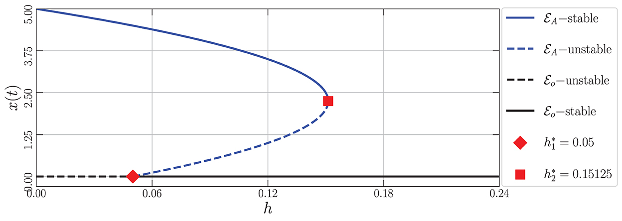
Figure 1. Bifurcation diagram driven by the harvesting rate (h) of the model (Equation 3) around the axial point using the parameter values: r = 0.1, K = 5, m = 0.25, c = 0.5, n = 0.01, β = 0.06, δ₁ = 0.05, δ₂ = 0.05, ω = 0.1, and α = 0.9.

FIGURE 2

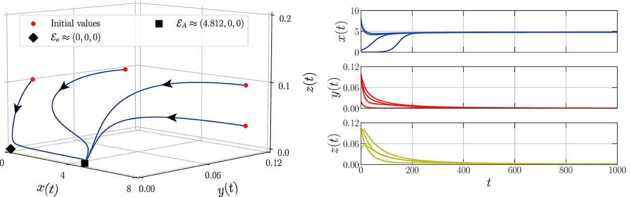
Figure 2. Phase portrait and time series of the model (Equation 3) using parameter values: r = 0.1, K = 5, m = 0.25, c = 0.5, n = 0.01, β = 0.06, δ₁ = 0.05, δ₂ = 0.05, ω = 0.1, α = 0.9, and h = 0.02.

FIGURE 3

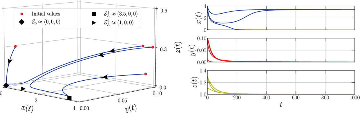
Figure 3. Phase portrait and time series of the model (Equation 3) using parameter values: r = 0.1, K = 5, m = 0.25, c = 0.5, n = 0.01, β = 0.06, δ₁ = 0.05, δ₂ = 0.05, ω = 0.1, α = 0.9, and h = 0.12.

FIGURE 4

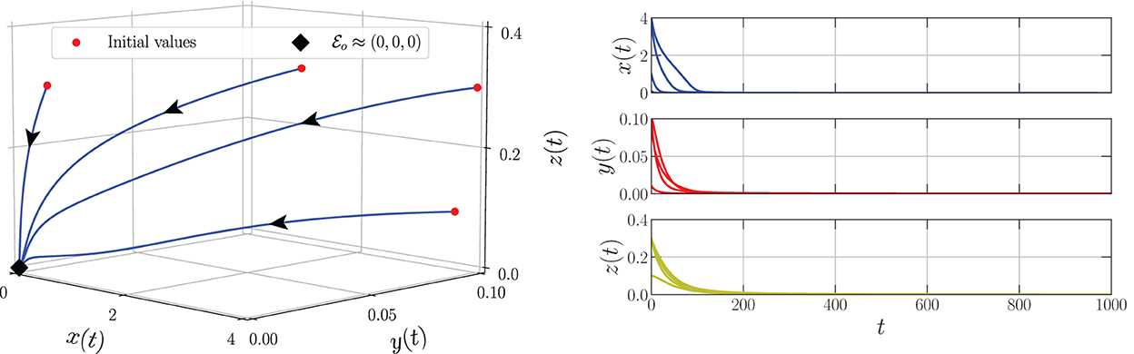
Figure 4. Phase portrait and time series of the model (Equation 3) using parameter values: r = 0.1, K = 5, m = 0.25, c = 0.5, n = 0.01, β = 0.06, δ₁ = 0.05, δ₂ = 0.05, ω = 0.1, α = 0.9, and h = 0.18.

From the biological point of view, these numerical bifurcations describe the possibility for the prey to extinct or survive due to the change in the harvesting rate while the predator both mature and immature is always extinct (Figure 1). Three feasible conditions may happen. First, for any sufficiently small harvesting rate ($0\le h<h_1^{*}=0.05$), the prey population may maintain its existence in this ecosystem (Figure 2). Second, if the harvesting rate increases ($h_1^{*}<h<h_2^{*}$), two possible conditions may occur namely the extinction of prey or the viability of prey. These circumstances depend on the initial condition, where if the initial condition is quite close to the origin point, the prey will be extinct, and for the initial condition is far enough from the origin point, the prey can survive extinction (Figure 3). Third, if the harvesting rate is again increased ($h>h_2^{*}$), the population of prey will finally extinct and there are no population again in this ecosystem (Figure 4).

The next circumstance occurs in the interior point of the model (Equation 3), which demonstrates the influence of the order of the derivative as the memory index on the dynamical behaviors around the interior point. We set the parameter as follows:

$\begin{array}{l}r=0.8,K=5,m=0.25,h=0.01,c=0.08,n=0.2,\\ \beta =0.4,{\delta }_1=0.01,{\delta }_2=0.01,{\delta }_2=0.01,\omega =0.1.& (26)\end{array}$

To identify the dynamical behaviors, we vary the values of α in the interval 0.76 ≤ α ≤ 1. As a result, we obtain the bifurcation diagram given in Figure 5. For α < α^* ≈ 0.86, the interior point ${{E}}_I$ is LAS. To show this condition, we give the phase portraits by selecting α = 0.81 and α = 0.84 as given in Figures 6A, B. Nearby solution oscillates and convergent to ${{E}}_I$. When α crosses α^* ≈ 0.86, ${{E}}_I$ losses its stability via Hopf bifurcation which is indicated by the occurrence of periodic signal namely limit-cycle. The nearby solution stays away from ${{E}}_I$ and convergent to the limit-cycle. The evolution of the limit-cycle given in Figure 5 also shows that the diameter of the limit-cycle increases when alpha increases. We portray the phase portraits in Figures 6C, D to show the dynamics of solutions around ${{E}}_I$ for α = 0.87 and α = 0.9. It is shown that the densities of all populations are oscillated and finally converge to the limit cycle. The physical interpretations of Hopf bifurcation driven by α are closely related to the influence of the memory on the change of behaviors around the interior point. The stronger the influence of memory, the higher the ability of prey and predators to maintain their existence (α < α^*). For less memory effect which is indicated by α > α^*, all populations lose the ability to stabilize their number of individuals. The population density fluctuates according to seasonal patterns which indicates by the appearance of a limit cycle (Figures 6C, D), and the peak of each population also increases for less memory effect (Figure 7). Although the density for each population cannot tend to a constant number, in this case, the memory effect cannot cause the extinction of every population.

FIGURE 5

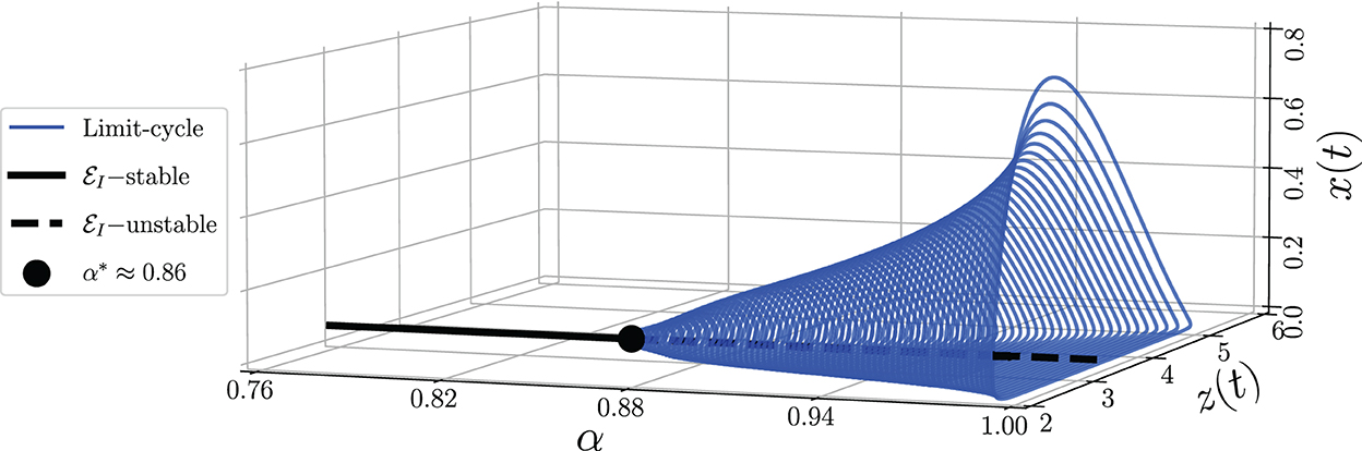
Figure 5. Bifurcation diagram driven by the order of the derivative (α) of model (Equation 3) around the axial point ${{E}}_I$ using parameter values: r = 0.8, K = 5, m = 0.25, h = 0.01, c = 0.08, n = 0.2, β = 0.4, δ₁ = 0.01, δ₂ = 0.01, δ₂ = 0.01, and ω = 0.1.

FIGURE 6

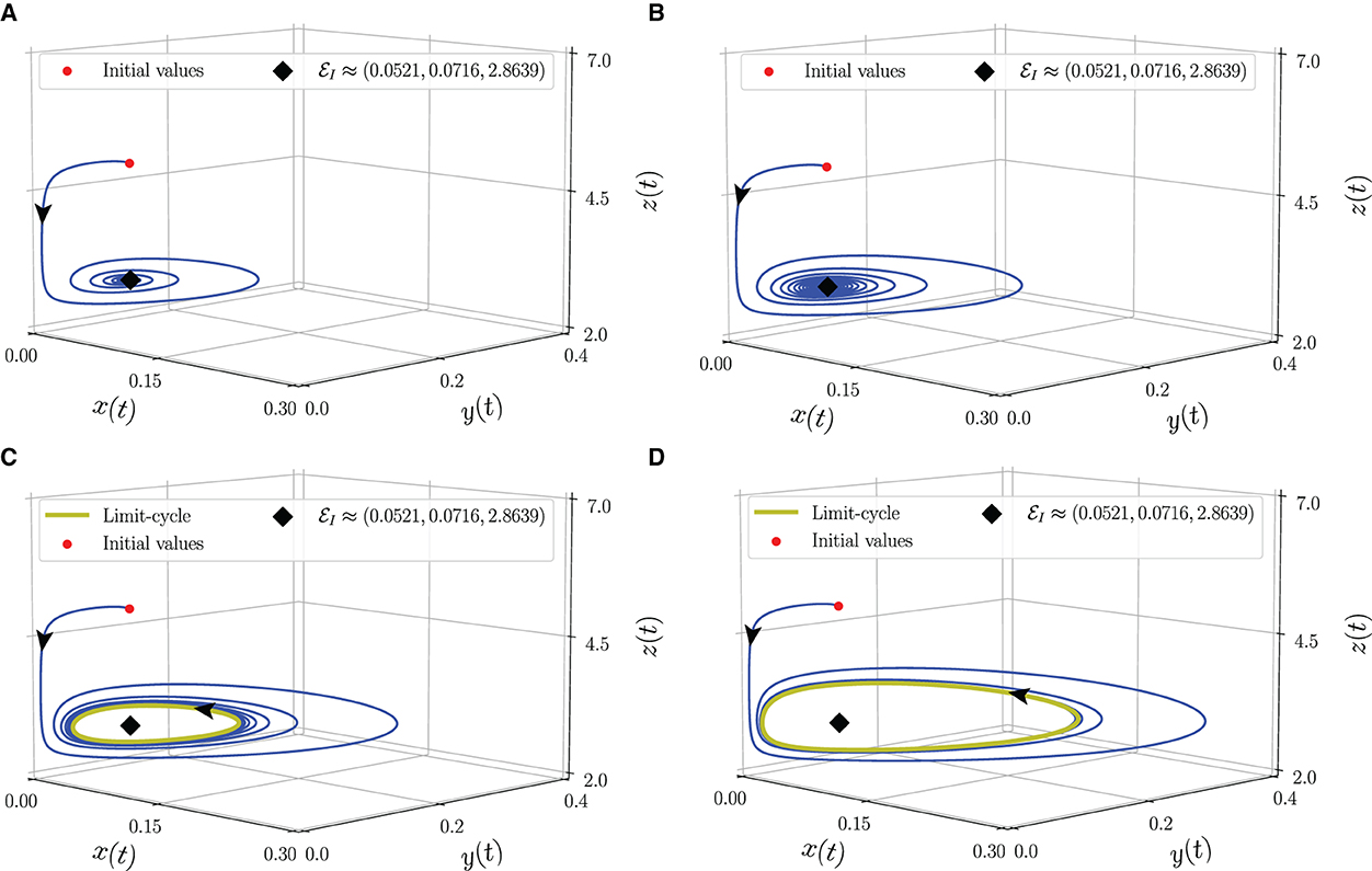
Figure 6. Phase portrait of the model (Equation 3) around interior point ${{E}}_I$ using parameter values from Equation (26). (A) α = 0.81, (B) α = 0.84, (C) α = 0.87, and (D) α = 0.9.

FIGURE 7

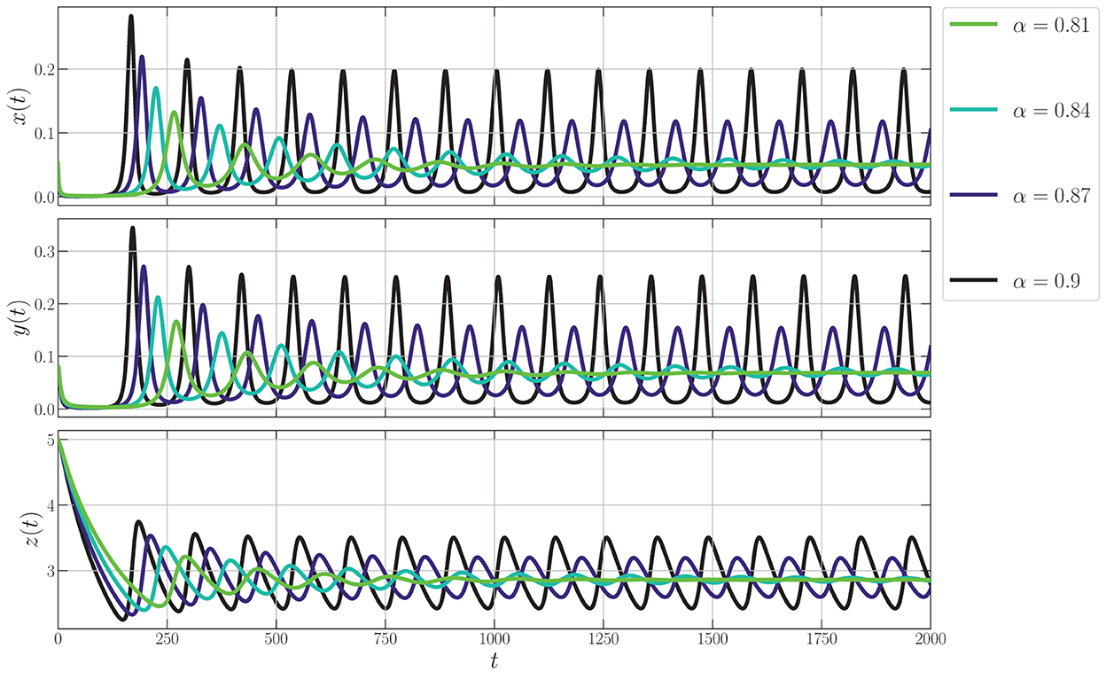
Figure 7. Phase portrait of the model (Equation 3) around interior point ${{E}}_I$ using parameter values from Equation (26).

7. Conclusion

The dynamics of a predator–prey model incorporating four biological conditions, namely age structure, intraspecific competition, Michaelis–Menten type harvesting, and memory effect, have been studied. All biological validities have been presented such as the existence, uniqueness, non-negativity, and boundedness of the solution. The dynamics of the model have been explored by showing the global stability conditions for three equilibrium points namely the origin, the axial, and the interior points. We have shown that three bifurcations phenomena driven by the harvesting rate occur around the axial point namely transcritical, saddle-node, and backward bifurcations. The bistability condition exists as the impact of saddle-node bifurcation which states that the existence of prey depends on the initial condition. A bifurcation driven by the memory effect also has been shown around the interior point which is called Hopf bifurcation. All the bifurcation phenomena having an impact on the densities of the population not only may reduce their densities but also threaten the existence of several populations.

Data availability statement

The original contributions presented in the study are included in the article/supplementary material, further inquiries can be directed to the corresponding author/s.

Author contributions

All authors listed have made a substantial, direct, and intellectual contribution to the work and approved it for publication.

Funding

This research was funded by LPPM-UNG via PNBP-Universitas Negeri Gorontalo according to DIPA-UNG No. 023.17.2.677521/2021, under contract No. B/176/UN47.DI/PT.01.03/2022.

Acknowledgments

The authors intended to express our gratitude and appreciation to the editors, reviewers, and all those who have supported us in improving this article.

Conflict of interest

The authors declare that the research was conducted in the absence of any commercial or financial relationships that could be construed as a potential conflict of interest.

Publisher's note

All claims expressed in this article are solely those of the authors and do not necessarily represent those of their affiliated organizations, or those of the publisher, the editors and the reviewers. Any product that may be evaluated in this article, or claim that may be made by its manufacturer, is not guaranteed or endorsed by the publisher.

References

1. Deng H, Chen F, Zhu Z, Li Z. Dynamic behaviors of Lotka-Volterra predator-prey model incorporating predator cannibalism. Adv Diff Equat. (2019) 2019:359. doi: 10.1186/s13662-019-2289-8

CrossRef Full Text | Google Scholar

2. Huang Q, Lin Y, Zhong Q, Ma F, Zhang Y. The impact of microplastic particles on population dynamics of predator and prey: implication of the Lotka-Volterra model. Sci Rep. (2020) 10:1–10. doi: 10.1038/s41598-020-61414-3

PubMed Abstract | CrossRef Full Text | Google Scholar

3. Tahara T, Gavina MKA, Kawano T, Tubay JM, Rabajante JF, Ito H, et al. Asymptotic stability of a modified Lotka-Volterra model with small immigrations. Sci Rep. (2018) 8:1–7. doi: 10.1038/s41598-018-25436-2

PubMed Abstract | CrossRef Full Text | Google Scholar

4. Zeng X, Liu L, Xie W. Existence and uniqueness of the positive steady state solution for a Lotka-Volterra predator-prey model with a crowding term. Acta Math Sci. (2020) 40:1961–80. doi: 10.1007/s10473-020-0622-7

CrossRef Full Text | Google Scholar

5. Gui Z, Ge W. The effect of harvesting on a predator-prey system with stage structure. Ecol Modell. (2005) 187:329–40. doi: 10.1016/j.ecolmodel.2005.01.052

CrossRef Full Text | Google Scholar

6. Magnússon KG. Destabilizing effect of cannibalism on a structured predator-prey system. Math Biosci. (1999) 155:61–75. doi: 10.1016/S0025-5564(98)10051-2

PubMed Abstract | CrossRef Full Text | Google Scholar

7. Liu C, Zhang Q, Huang J. Stability analysis of a harvested prey-predator model with stage structure and maturation delay. Math Problems Eng. (2013) 2013:329592. doi: 10.1155/2013/329592

CrossRef Full Text | Google Scholar

8. Dubey B, Agarwal S, Kumar A. Optimal harvesting policy of a prey-predator model with Crowley-Martin-type functional response and stage structure in the predator. Nonlinear Anal Model Control. (2018) 23:493–514. doi: 10.15388/NA.2018.4.3

CrossRef Full Text | Google Scholar

9. Xiao Z, Li Z, Zhu Z, Chen F. Hopf bifurcation and stability in a Beddington-DeAngelis predator-prey model with stage structure for predator and time delay incorporating prey refuge. Open Math. (2019) 17:141–59. doi: 10.1515/math-2019-0014

CrossRef Full Text | Google Scholar

10. Zhang X, Liu Z. Periodic oscillations in age-structured ratio-dependent predator-prey model with Michaelis-Menten type functional response. Physica D. (2019) 389:51–63. doi: 10.1016/j.physd.2018.10.002

CrossRef Full Text | Google Scholar

11. Zhang F, Chen Y, Li J. Dynamical analysis of a stage-structured predator-prey model with cannibalism. Math Biosci. (2019) 307:33–41. doi: 10.1016/j.mbs.2018.11.004

PubMed Abstract | CrossRef Full Text | Google Scholar

12. Lu W, Xia Y. Periodic solution of a stage-structured predator-prey model with Crowley-Martin type functional response. AIMS Math. (2022) 7:8162–75. doi: 10.3934/math.2022454

CrossRef Full Text | Google Scholar

13. Li J, Liu X, Wei C. The impact of role reversal on the dynamics of predator-prey model with stage structure. Appl Math Model. (2022) 104:339–57. doi: 10.1016/j.apm.2021.11.029

CrossRef Full Text | Google Scholar

14. Wang W, Chen L. A predator-prey system with stage-structure for predator. Comput Math Appl. (1997) 33:83–91. doi: 10.1016/S0898-1221(97)00056-4

CrossRef Full Text | Google Scholar

15. Chow C, Hoti M, Li C, Lan K. Local stability analysis on Lotka-Volterra predator-prey models with prey refuge and harvesting. Math Methods Appl Sci. (2018) 41:7711–32. doi: 10.1002/mma.5234

CrossRef Full Text | Google Scholar

16. Xiao M, Cao J. Hopf bifurcation and non-hyperbolic equilibrium in a ratio-dependent predator-prey model with linear harvesting rate: analysis and computation. Math Comput Model. (2009) 50:360–79. doi: 10.1016/j.mcm.2009.04.018

CrossRef Full Text | Google Scholar

17. Zhang Z, Upadhyay RK, Datta J. Bifurcation analysis of a modified Leslie-Gower model with Holling type-IV functional response and nonlinear prey harvesting. Adv Diff Equat. (2018) 2018:127. doi: 10.1186/s13662-018-1581-3

CrossRef Full Text | Google Scholar

18. Mulheisen M, Allen C, Parr CS. Lycaon Pictus. (On-line), Animal Diversity Web. (2002). Available online at: https://animaldiversity.org/accounts/Lycaon_pictus/ (accessed on November 13, 2022)

19. IUCN SSC Antelope Specialist Group. Aepyceros melampus. The IUCN Red List of Threatened Species 2016: eT550A50180828. (2016). Available online at: https://www.iucnredlist.org/species/550/50180828 (accessed on November 13, 2022)

20. Huo J, Zhao H, Zhu L. The effect of vaccines on backward bifurcation in a fractional order HIV model. Nonlinear Anal. Real World Appl. (2015) 26:289–305. doi: 10.1016/j.nonrwa.2015.05.014

CrossRef Full Text | Google Scholar

21. Moustafa M, Mohd MH, Ismail AI, Abdullah FA. Stage structure and refuge effects in the dynamical analysis of a fractional order Rosenzweig-MacArthur prey-predator model. Progr Fract Different Appl. (2019) 5:49–64. doi: 10.18576/pfda/050106

CrossRef Full Text | Google Scholar

22. Rahmi E, Darti I, Suryanto A, Trisilowati, Panigoro HS. Stability analysis of a fractional-order leslie-gower model with allee effect in predator. J Phys. (2021) 1821:012051. doi: 10.1088/1742-6596/1821/1/012051

CrossRef Full Text | Google Scholar

23. Owolabi KM. Dynamical behaviour of fractional-order predator-prey system of Holling-type. Discrete Contin Dyn Syst S. (2020) 13:823–34. doi: 10.3934/dcdss.2020047

CrossRef Full Text | Google Scholar

24. Barman D, Roy J, Alam S. Modelling hiding behaviour in a predator-prey system by both integer order and fractional order derivatives. Ecol Inform. (2022) 67:101483. doi: 10.1016/j.ecoinf.2021.101483

CrossRef Full Text | Google Scholar

25. Ghanbari B, Djilali S. Mathematical and numerical analysis of a three-species predator-prey model with herd behavior and time fractional-order derivative. Math Methods Appl Sci. (2020) 43:1736–52. doi: 10.1002/mma.5999

CrossRef Full Text | Google Scholar

26. Yousef FB, Yousef A, Maji C. Effects of fear in a fractional-order predator-prey system with predator density-dependent prey mortality. Chaos Solitons Fractals. (2021) 145:110711. doi: 10.1016/j.chaos.2021.110711

CrossRef Full Text | Google Scholar

27. Ghosh U, Pal S, Banerjee M. Memory effect on Bazykin's prey-predator model: stability and bifurcation analysis. Chaos Solitons Fractals. (2021) 143:110531. doi: 10.1016/j.chaos.2020.110531

CrossRef Full Text | Google Scholar

28. Panigoro HS, Rahmi E, Achmad N, Mahmud SL, Resmawan R, Nuha AR. A discrete-time fractional-order rosenzweig-macarthur predator-prey model involving prey refuge. Commun Math Biol Neurosci. (2021) 2021:1–19. doi: 10.28919/cmbn/6586

CrossRef Full Text | Google Scholar

29. Panigoro HS, Resmawan R, Sidik ATR, Walangadi N, Ismail A, Husuna C. A fractional-order predator-prey model with age structure on predator and nonlinear harvesting on prey. Jambura J Math. (2022) 4:355–66. doi: 10.34312/jjom.v4i2.15220

CrossRef Full Text | Google Scholar

30. Mahata A, Paul S, Mukherjee S, Das M, Roy B. Dynamics of caputo fractional order SEIRV epidemic model with optimal control and stability analysis. Int J Appl Comput Math. (2022) 8:1–25. doi: 10.1007/s40819-021-01224-x

PubMed Abstract | CrossRef Full Text | Google Scholar

31. Yavuz M, Sene N. Stability analysis and numerical computation of the fractional predator-prey model with the harvesting rate. Fractal Fract. (2020) 4:35. doi: 10.3390/fractalfract4030035

CrossRef Full Text | Google Scholar

32. Maji C. Impact of fear effect in a fractional-order predator-prey system incorporating constant prey refuge. Nonlinear Dyn. (2022) 107:1329–42. doi: 10.1007/s11071-021-07031-9

CrossRef Full Text | Google Scholar

33. Barman D, Roy J, Alrabaiah H, Panja P, Mondal SP, Alam S. Impact of predator incited fear and prey refuge in a fractional order prey predator model. Chaos Solitons Fractals. (2021) 142:110420. doi: 10.1016/j.chaos.2020.110420

CrossRef Full Text | Google Scholar

34. Panigoro HS, Suryanto A, Kusumahwinahyu WM, Darti I. Dynamics of a fractional-order predator-prey model with infectious diseases in prey. Commun Biomath Sci. (2019) 2:105. doi: 10.5614/cbms.2019.2.2.4

CrossRef Full Text | Google Scholar

35. Vargas-De-León C. Volterra-type Lyapunov functions for fractional-order epidemic systems. Commun Nonlinear Sci Num Simulat. (2015) 24:75–85. doi: 10.1016/j.cnsns.2014.12.013

CrossRef Full Text | Google Scholar

36. Aguila-Camacho N, Duarte-Mermoud MA, Gallegos JA. Lyapunov functions for fractional order systems. Commun Nonlinear Sci Num Simulat. (2014) 19:2951–7. doi: 10.1016/j.cnsns.2014.01.022

PubMed Abstract | CrossRef Full Text | Google Scholar

37. Diethelm K, Ford NJ, Freed AD. A predictor-corrector approach for the numerical solution of fractional differential equations. Nonlinear Dyn. (2002) 29:3–22. doi: 10.1023/A:1016592219341

CrossRef Full Text | Google Scholar

38. Adhikary PD, Mukherjee S, Ghosh B. Bifurcations and hydra effects in Bazykin's predator-prey model. Theor Populat Biol. (2021) 140:44–53. doi: 10.1016/j.tpb.2021.05.002

PubMed Abstract | CrossRef Full Text | Google Scholar