Dynamical solutions and quadratic resonance of nonlinear perturbed Schrödinger equation

1. Introduction

Nonlinear evolution equations (NLEEs) are used to explain various nonlinear conflicts and problems seen in different branches of science, such as plasma physics, optical fiber communication, fluid dynamics, population growth dynamics, water waves, chaos theory, and others [1–5]. Therefore, a large number of studies have been adopted on improved new methods or some modifications to well-established methods to derive new analytical solutions that can successfully describe certain complicated physical approaches. From the literature of applied mathematics and associated areas of nonlinear science, efforts have increased to obtain traveling wave solutions of NLEEs, which provide momentous physical properties and akin information. Thus, many powerful and efficient methods have been developed to find analytical solutions for traveling waves, such as the tanh-function method [6, 7], variational iteration algorithm-II [8], $(\frac{G^{\prime }}{G})$-expansion method [9–11], $(\frac{G^{\prime }}{G},\frac{1}{G})$-expansion method [12], first integral method [13], simplest equation method [14, 15], Kudryashov method [16, 17], modified simple equation method [18], extended rational sine-cosine method [19], modified $(\frac{G^{\prime }}{G^2})$-expansion method [20, 21], sine-cosine method [22], and so on.

From the literature, some methods from the family of $(\frac{G^{\prime }}{G})$-expansion method have been extensively used to finding the exact solutions of NLEEs, such as the $(\frac{1}{G^{\prime }})$-expansion method, double $(\frac{G^{\prime }}{G},\frac{1}{G})$-expansion method, extended $(\frac{G^{\prime }}{G})$-expansion method, improved $(\frac{G^{\prime }}{G})$-expansion method, and modified $(\frac{G^{\prime }}{G})$-expansion method. In addition these methods, Li et al. introduced another novel method, the $(\frac{w}{g})$-expansion method [23], where w and g satisfy the relation as follows:

$\begin{array}{ll}{\left(\frac{w}{g}\right)}^{\prime }=\sigma +\mu \left(\frac{w}{g}\right)+\rho {\left(\frac{w}{g}\right)}^2,& (1)\end{array}$

Where σ, μ, and ρ represent some constants. Considering suitable values of w and g, the aforementioned relation leads to $(\frac{G^{\prime }}{G})$-expansion method, tanh method, or $(\frac{G^{\prime }}{G^2})$-expansion method. Later, method can be realized when $w=(\frac{G^{\prime }}{G})$ and g = G. This method has been successfully implemented to find out exact solutions of some nonlinear problems in mathematical physics.

In this research work, the authors considered the extended version of the $\frac{w}{g}$-expansion method, namely modified $(\frac{G^{\prime }}{G^2})$-expansion method when w and g satisfy

$\begin{array}{ll}{w}^{\prime }g-w{g}^{\prime }\sigma g^2+\mu wg+\rho w^2,& (2)\end{array}$

considering μ ≠ 0, $w=(\frac{G^{\prime }}{G})$ and g = G leads to

$\begin{array}{ll}{G}^{″}G-2G^{\prime }{G}^2=\sigma {G{}^{\prime }}^2+\mu G^{\prime }{G}^2+\rho G^4,& (3)\end{array}$

Furthermore, the explicit expressions for novel exact solutions of the considered NLEEs are propped by considering the general solutions of Equation (3). The focused modified method gives abundant exact solutions to a class of NLEEs. More number of novel and unique solutions are realized by this method over other conventional methods, is one of its major advantage. The nonlinear perturbed Schrödinger equation has been focused on across a significant amount of research by a variety of authors. The PNSE have been studied by using different methods, for instance, the tanh method, $(\frac{G^{\prime }}{G})$-expansion method, rational hyperbolic method, and so on. To describe the effectiveness of the proposed method and to find out the exact traveling wave solutions, PNSE will be considered. The method is mathematically concise, direct, and more effective in constructing the explicit traveling wave solutions of NLEEs.

2. The modified $(\frac{G^{\prime }}{G^2})$-expansion method

In this section, we outline the general facts of the modified $(\frac{G^{\prime }}{G^2})$-expansion method [24].

Step 1: A NLEE may be sometimes expressed as

$\begin{array}{ll}s\left(f,f_t,f_x,f_{tt},f_{xt},f_{xx},...\right)=0,& (4)\end{array}$

by utilizing the wave transformation ϕ = x − Vt and wave variable f(x, t) = F(ϕ) where F(ϕ) is a trial function. Immediately, the following changes can be implemented.

$\begin{array}{l}\frac{\partial }{\partial t}=-V\frac{\partial }{\partial \varphi },\frac{{\partial }^2}{\partial t^2}=V^2\frac{{\partial }^2}{\partial {\varphi }^2},\frac{\partial }{\partial x}=\frac{\partial }{\partial \varphi },\frac{{\partial }^2}{\partial x^2}\\ =\frac{{\partial }^2}{\partial {\varphi }^2},& (5)\end{array}$

Equation (4) can be transformed into an ordinary differential equation (ODE)

$\begin{array}{ll}S\left(F,F_{\varphi },F_{\varphi \varphi },F_{\varphi \varphi \varphi },...\right)=0,& (6)\end{array}$

Where S is the polynomial in F and successive derivatives of F. F_ϕ denotes $\frac{dF}{d\varphi }$ and V is the speed of wave. In case all the terms involved with derivatives, we can integrate the obtained ordinary differential equation (ODE) (Equation 6). Furthermore, by considering F → 0 as ϕ → ∞, the integration constant can be equated to zero.

Step 2: Taking the formal solution of ODE (Equation 6)

$\begin{array}{ll}F\left(\varphi \right)=a_0+{\displaystyle \sum _{n=1}^N}\left\{a_n{\left(\frac{G^{\prime }}{G^2}\right)}^n+b_n{\left(\frac{G^{\prime }}{G^2}\right)}^{-n}\right\},& (7)\end{array}$

Where a₀, a_n, and b_n(n = 1, 2, 3, .... N) are some constants, and G = G(ϕ) satisfies

$\begin{array}{ll}{\left(\frac{G^{\prime }}{G^2}\right)}^{\prime }=\sigma +\mu \left(\frac{G^{\prime }}{G^2}\right)+\rho {\left(\frac{G^{\prime }}{G^2}\right)}^2,& (8)\end{array}$

Where μ, σ, and ρ are free parameters. The positive integer N can be found out by the balance principle between the nonlinear term and the highest order derivatives terms involved in Equation (6). Substitution of Equation (7), and its derivatives along with Equation (8) into Equation (6). We will have a complex system, collecting the exponents with the same power of $(\frac{G^{\prime }}{G^2})$, and then setting them zero separately, we will get systems of algebraic equations for a₀, a_n,b_n, and (n = 1, 2, 3, ....). Solving these systems, we shall determine σ, μ, and ρ, and values of a₀, a_n,b_n, and (n = 1, 2, 3, ....)

Step 3: There will be five generalized solutions of Equation (5).

Case 1: (Trigonometric solution)

when σ ρ > 0, μ = 0

$\begin{array}{ll}(\frac{G^{\prime }}{G^2})=\frac{\sqrt{\sigma \rho }}{\sigma }\left[\frac{A_{1}cos\sqrt{\sigma \rho }\varphi +A_{2}sin\sqrt{\sigma \rho }\varphi }{A_{1}sin\sqrt{\sigma \rho }\varphi -A_{2}cos\sqrt{\sigma \rho }\varphi }\right],& (9)\end{array}$

Case 2: (Hyperbolic solution)

when σ ρ < 0, μ = 0

$\begin{array}{l}(\frac{G^{\prime }}{G^2})=-\frac{\sqrt{\left|\sigma \rho \right|}}{\rho }\\ \left[\frac{A_{1}sinh2\sqrt{\left|\sigma \rho \right|}\varphi +A_{2}cosh2\sqrt{\left|\sigma \rho \right|}\varphi +A_2}{A_{1}cosh2\sqrt{\left|\sigma \rho \right|}\varphi +A_{1}sinh2\sqrt{\left|\sigma \rho \right|}\varphi -A_2}\right]& (10)\end{array}$

Case 3: (Rational solution)

when σ = 0, ρ ≠ 0, μ = 0

$\begin{array}{ll}(\frac{G^{\prime }}{G^2})=-\frac{A_1}{\rho \left(A_1\varphi +A_2\right)},& (11)\end{array}$

Case 4: (Hyperbolic solution)

when μ ≠ 0, △₁ ≥ 0 and ${△}_1={\mu }^2-4\sigma \rho$

$\begin{array}{l}(\frac{G^{\prime }}{G^2})=-\frac{\mu }{2\rho }\\ -\left[\frac{\sqrt{{△}_1}(A_{1}cosh(\frac{\sqrt{{△}_1}}{2})\varphi +A_{2}sinh(\frac{\sqrt{{△}_1}}{2})\varphi )}{2\rho (A_{1}cosh(\frac{\sqrt{{△}_1}}{2})\varphi +A_{2}sinh(\frac{\sqrt{{△}_1}}{2})\varphi )}\right],& (12)\end{array}$

Case 5: (Hyperbolic solution)

when μ ≠ 0, △₂ ≥ 0 and ${△}_2=4\sigma \rho -{\mu }^2$

$\begin{array}{l}(\frac{G^{\prime }}{G^2})=-\frac{\mu }{2\rho }\\ -\left[\frac{\sqrt{{△}_2}(A_{1}cosh(\frac{\sqrt{{△}_2}}{2})\varphi -A_{2}sinh(\frac{\sqrt{{△}_2}}{2})\varphi )}{2\rho (A_{1}cosh(\frac{\sqrt{{△}_2}}{2})\varphi +A_{2}sinh(\frac{\sqrt{{△}_2}}{2})\varphi )}\right],& (13)\end{array}$

where A₁ and A₂ are constants.

Remark 1: More (five cases) analytical solutions are reported in the proposed method as compared to the basic $(\frac{G^{\prime }}{G^2})$-expansion method (three cases) [23, 24].

Remark 2: More free parameters are involved in our proposed method as compared to the basic $(\frac{G^{\prime }}{G^2})$-expansion method [23, 24].

3. Nonlinear perturbed Schrödinger equation

The modified $(\frac{G^{\prime }}{G^2})$-expansion method has been implemented to perceive analytical solutions of the nonlinear perturbed Schrödinger equation (NPSE) is written as follows:

$\begin{array}{ll}i{f}_t+f_{xx}+\alpha f|f{|}^2+i[{\gamma }_1{f}_{xxx}+{\gamma }_2|f{|}^2{f}_x+{\gamma }_{3}f{(|f{|}^2)}_x]=0& (14)\end{array}$

Where α, γ₁, γ₂, and γ₃ are constants. In Zhang [25] obtained the Jacobi elliptic function solutions of Equation (14) by using a modified mapping method. In Shehata [26] has been utilized a modified $(\frac{G}{G^{\prime }})$-expansion method, and analytical solutions have been realized. Different forms of these equations have some particular properties and use in communications of optical soliton. Their pulse center, width, and amplitude can be adjusted while propagating in corresponding with the structural constraints, such as line gain, nonlinearity, and diffusion [27]. The general form of NPSE reads as follows:

$\begin{array}{ll}i{f}_t+\frac{1}{2}{f}_{xx}+\alpha f|f{|}^2=iϵR[f,f^{*}]& (15)\end{array}$

When R[f, f^*] = 0, the dimensionless, non-Kerr law nonlinear Schrödinger equation and similarly for αf|f|² = |f|² and R[f, f^*] = 0, Kerr law nonlinear Schrödinger equation is realized from Equation (15). The first term of the left-hand side of the aforementioned equation is the evolution term, and the second one is the group velocity dispersion (GVD) term. On the right-hand side, R is the spatio-differential or integro-differential operator, and ϵ is the perturbation parameter with 0 < ϵ ≤ 0, sometimes termed as the relative width of the quasi-monochromaticity spectrum [28]. While the perturbed terms are as follows:

$\begin{array}{ll}\begin{array}{c}R=\delta |f{|}^{2m}f+\alpha f_x+\beta f_{xx}-\gamma f_{xxx}+\lambda {(|f{|}^{2}f)}_x+\theta {(|f{|}^2)}_{x}f\hfill \\ +\rho (|f_x{|}^{2}f)-i\xi {(f^2{f}_x^{*})}_x-i\eta f_x^2{f}^{*}\hfill \\ -i\zeta f^{*}{(f^2)}_{xx}-i\mu {(|f{|}^2)}_{x}f-i\chi f_{xxxx}-i\psi f_{xxxxxx}\hfill \\ +({\sigma }_{1}f+{\sigma }_2{f}_x){\displaystyle {\int }_{-\infty }^{\infty }}|f{|}^{2}ds.\hfill \end{array}\hfill & (16)\end{array}$

Where δ in the first term is either coefficient of nonlinear damping or amplification factor based on the sign and m can take values 0, 1, and 2. It will be linear amplification or attenuation depending on its positive or negative signs, respectively, provided m = 0. Two-photon absorption or a complex nonlinear gain could be realized when m = 1 and δ is a positive quantity. In contrast, higher-order loss or saturation correction term arises when m=2. Frequency separation term α basically intervenes with the frequency of EDFA gain at its peak and the soliton carrier. Here, β represents the bandpass filtering and λ stands for self-steeping coefficients in the short pulse range. θ and ρ are nonlinear dispersion terms. The perturbed coefficients of ξ, η, and ζ come to light because of quasi-solitons, μ stands for the coefficient of Raman scattering, and γ, χ, and ψ are coefficients of higher-order dispersions, whereas σ₁ and σ₂ are two perturbed integro-differential terms due to saturable amplifiers. Equation (15) is a special case of Equation (14) and is popularly known as nonlinear Schrödinger equation (NLSE). For smaller pulses such as solitary lasers in solid state physics having a pulse width of 10 fs, which is smaller than the critical value 1 ps, correct prediction no longer holds good, and the approximation breaks down. In this context, quasi-monochromaticity is violated, and the importance of higher-order dispersion terms comes into the picture. When GVD approaches zero to enhance the performance along with trans-oceanic and trans-continental distances, it is mandatory to receive the third and higher-order dispersions. Furthermore, in case of short pulse widths where GVD changes randomly, reference to the spectral bandwidth of the signal cannot be neglected and it is obvious to depend on higher-order dispersion terms. That is why the coefficients of χ and ψ are included in Equation (16) for the fourth and sixth order dispersion terms, respectively.

Studies on the NPSE by different methods flourish some important features and properties. The soliton pulses are the result of a perfect balance between dispersion effects and nonlinearity, the soliton interaction, symmetry analysis, integrability, and other useful concepts and physical applications are among notable features that attracted research scientists from all over the globe.

A few years after Equation (14) was proposed, a plethora of results about its exact traveling solutions is being constantly reported. In this study, we use the modified $(\frac{G^{\prime }}{G^2})$-expansion method to study the exact solution of Equation (14). By considering the complex wave transformation f(x, t) = F(ϕ)exp(iη), where ϕ = k(x − ct), η = (λx − wt) provided λ, w, k, and c are constants, when the real and imaginary parts are embedded separately canceling the common term exp(iη), the NPSE (14) is reduced to the following form of F(ϕ):

$\begin{array}{ll}{k}^2(1-3{\gamma }_1\lambda )F^{″}+(w-{\lambda }^2+{\gamma }_1{\lambda }^3)F+(\alpha -{\gamma }_2\lambda )F^3=0& (17)\end{array}$

and

$\begin{array}{ll}{\gamma }_1{k}^2{F}^{‴}-(c-2\lambda +3{\gamma }_1{\lambda }^2)F^{\prime }+({\gamma }_2+2{\gamma }_3)F^2{F}^{\prime }=0& (18)\end{array}$

Integrating the aforementioned Equation (18) with respect to ϕ and considering the integration constant as zero, we have developed

$\begin{array}{ll}{\gamma }_1{k}^2{F}^{″}+(2\lambda -c+3{\gamma }_1{\lambda }^2)F+(\frac{1}{3}{\gamma }_2+\frac{2}{3}{\gamma }_3)F^3=0& (19)\end{array}$

4. Quadratic resonance

In a way to outcast the quadratic term ($i[{\gamma }_1{f}_{xxx}+{\gamma }_2|f{|}^2{f}_x+{\gamma }_{3}f{(|f{|}^2)}_x]$) of Equation (18), we can analyze the quadratic resonance in the linear form of the NPSE

$\begin{array}{ll}i{f}_t+f_{xx}+\alpha f|f{|}^2=0,& (20)\end{array}$

Substitution of f = e^i(kx+λt), we can realize the dispersion relation of the Equation (20), and the mathematical structure is given by

$\begin{array}{ll}\lambda =ik\sqrt{k^2-w^2},k=\pm 1,\pm 2,...& (21)\end{array}$

Literally, the meaning of quadratic resonance stands for nonzero integer values of k, such that

$\begin{array}{ll}{k}_1=k_2+k_3& (22)\end{array}$

$\begin{array}{ll}{\lambda }_1\pm {\lambda }_2=\pm {\lambda }_3& (23)\end{array}$

Resonance condition can be verified by squaring Equation (23) and submitting in Equation (22), we have

$\begin{array}{ll}2k_1^2+3k_1{k}_2+2k_2^2-4w^2=\pm \sqrt{k_1^2-4w^2}\sqrt{k_2^2-4w^2}& (24)\end{array}$

Again squaring the aforementioned equation, we have

$\begin{array}{ll}[{(k_1+k_2)}^2+k_1^2+k_2^2-6w^2]{(k_1+k_2)}^2=0& (25)\end{array}$

When k₁ + k₂ = k₃ = 0, the equation will be valid.

5. Dispersion relation

In the case of weak nonlinearity, Zakharov and Shabat in the year 1972 [29] and Ablowitz et al. in the year 1974 [30] shown separately from any initial condition f(x, t = 0) will tend to be zero as |x| → ∞ and as a result, an envelope soliton will be formed. When the spread of the soliton only depends upon the initial condition, i.e., phase and temporal range, depending on the w value, either dark or bright soliton will be realized. For example, by putting k = 3 in the dispersion relation, Equation (21) a bright soliton will propagate that leads it, whereas at k = −3, a soliton will propagate that follows it.

From Equation (17) and Equation (19), it is obvious that the coefficients of both equations for a real function F = F(ϕ) must satisfy the well-known proportionality relation,

$\begin{array}{ll}\frac{{\gamma }_1}{(1-3{\gamma }_1\lambda )}=\frac{(2\lambda -c+3{\gamma }_1{\lambda }^2)}{(w-{\lambda }^2+{\gamma }_1{\lambda }^3)}=\frac{(\frac{1}{3}{\gamma }_2+\frac{2}{3}{\gamma }_3)}{(\alpha -{\gamma }_2\lambda )},& (26)\end{array}$

After some mathematical simplification

$\begin{array}{ll}w=\frac{(\alpha -{\gamma }_2\lambda )(2\lambda -c+3{\gamma }_1{\lambda }^2)}{(\frac{1}{3}{\gamma }_2+\frac{2}{3}{\gamma }_3)}+{\lambda }^2-{\gamma }_1{\lambda }^3,& (27)\end{array}$

here,

$\begin{array}{ll}\lambda =\frac{{\gamma }_2+2{\gamma }_3-3\alpha {\gamma }_1}{({\gamma }_2+2{\gamma }_3){\lambda }_1-3{\gamma }_1{\gamma }_2}.& (28)\end{array}$

According to the aforementioned proportionality relation, Equation (17) or Equation (19) can be solved in lieu of both the Equations (17) and (19), only if the Equation (17) and Equation (19) are written in terms of Equations (27) and (28), respectively. Let,

$\begin{array}{ll}A={\gamma }_1{k}^2,B=2\lambda -c-3{\gamma }_1{\lambda }^2,D=\left(\frac{1}{3}{\gamma }_2+\frac{2}{3}{\gamma }_3\right).& (29)\end{array}$

Now Equation (17) can be restructured into a simpler form

$\begin{array}{ll}A{F}^{″}+BF+D{F}^3=0.& (30)\end{array}$

By using the homogeneous balance method between F″ and F³ in Equation (7), we obtain N = 1. Therefore, from Equation (7), the formal solution has the following form:

$\begin{array}{ll}F(\varphi )=a_0+a_1{\left(\frac{G^{\prime }}{G^2}\right)}^1+b_1{\left(\frac{G^{\prime }}{G^2}\right)}^{-1}& (31)\end{array}$

Collecting all the terms in accordance with the same powers of $(\frac{G^{\prime }}{G^2})$ and equating them separately to zero by substituting Equation (31) into Equation (30) along with Equation (8), yields an algebraic simultaneous equation set for a₀, a₁, b₁, μ, σ, and ρ, and after solving them, we have the following values:

$\begin{array}{l}{a}_0=-\frac{i\sqrt{B}}{\sqrt{D}},a_1=0,b_1=\frac{i\sqrt{B}}{\sqrt{D}},\sigma =-\frac{\sqrt{B}}{\sqrt{2}\sqrt{A}},\\ \mu =\frac{\sqrt{2}\sqrt{B}}{\sqrt{A}},\rho =\rho & (32)\end{array}$

Analytical solutions:

Case 1: The trigonometric solution of Equation (14) by the use of Equation (9) and under the parametric value of Equation (9) can be given as follows:

$\begin{array}{l}{F}_1(\varphi )=-\frac{i\sqrt{B}}{\sqrt{D}}+\frac{i\sqrt{B}}{\sqrt{D}}\sqrt{-\frac{\sqrt{B}}{\rho \sqrt{2}\sqrt{A}}}\\ {\left(\frac{A_{1}cos(-\frac{\rho \sqrt{B}}{\sqrt{2}\sqrt{A}})\varphi +A_{2}sin(-\frac{\rho \sqrt{B}}{\sqrt{2}\sqrt{A}})\varphi }{A_{1}sin(-\frac{\rho \sqrt{B}}{\sqrt{2}\sqrt{A}})\varphi -A_{2}cos(-\frac{\rho \sqrt{B}}{\sqrt{2}\sqrt{A}})\varphi }\right)}^{-1}& (33)\end{array}$

Case 2: The hyperbolic solution of Equation (14) by the use of Equation (10) and under the parametric value of Equation (33) can be given as follows:

$\begin{array}{l}{F}_2(\varphi )=\frac{i\sqrt{B}}{\sqrt{D}}++\frac{i\sqrt{B}}{\rho \sqrt{D}}\left(\sqrt{|(-\frac{\rho \sqrt{B}}{\sqrt{2}\sqrt{A}})|}\right)\\ {\left(\frac{A_{1}sinh2(\sqrt{|(-\frac{\rho \sqrt{B}}{\sqrt{2}\sqrt{A}})|})\varphi +A_{1}cosh2(\sqrt{|(-\frac{\rho \sqrt{B}}{\sqrt{2}\sqrt{A}})|})\varphi +A_2}{A_{1}sinh2(\sqrt{|(-\frac{\rho \sqrt{B}}{\sqrt{2}\sqrt{A}})|})\varphi -A_{1}cosh2(\sqrt{|(-\frac{\rho \sqrt{B}}{\sqrt{2}\sqrt{A}})|})\varphi -A_2}\right)}^{-1}& (34)\end{array}$

Case 3: The rational solution of Equation (14) by the use of Equation (11) and under the parametric value of Equation (32) can be given as follows:

$\begin{array}{ll}{F}_3(\varphi )=-\frac{i\sqrt{B}}{\sqrt{D}}+\frac{i\sqrt{B}}{\sqrt{D}}{\left(\frac{A_1}{\rho (A_1\varphi +A_2)}\right)}^{-1}& (35)\end{array}$

Case 4: The hyperbolic solution of Equation (14) by the use of Equation (12) and under the parametric value of Equation (32) can be given as follows:

$\begin{array}{l}{F}_4(\varphi )=-\frac{i\sqrt{B}}{\sqrt{D}}+\frac{i\sqrt{B}}{\sqrt{D}}\\ {\left[-\frac{\sqrt{2}\sqrt{B}}{2\rho \sqrt{A}}-\left(\frac{\sqrt{{△}_1}(A_{1}cosh(\frac{\sqrt{{△}_1}}{2})\varphi +A_{2}sinh(\frac{\sqrt{{△}_1}}{2})\varphi )}{2\rho (A_{1}cosh(\frac{\sqrt{{△}_1}}{2})\varphi +A_{2}sinh(\frac{\sqrt{{△}_1}}{2})\varphi )}\right)\right]}^{-1},& (36)\end{array}$

Case 5: The hyperbolic solution of Equation (14) by the use of Equation (13) and under the parametric value of Equation (32) can be given as follows:

$\begin{array}{l}{F}_5(\varphi )=-\frac{i\sqrt{B}}{\sqrt{D}}+\frac{i\sqrt{B}}{\sqrt{D}}\\ {\left[-\frac{\sqrt{2}\sqrt{B}}{2\rho \sqrt{A}}-\left(\frac{\sqrt{{△}_2}(A_{1}cosh(\frac{\sqrt{{△}_2}}{2})\varphi -A_{2}sinh(\frac{\sqrt{{△}_2}}{2})\varphi )}{2\rho (A_{1}cosh(\frac{\sqrt{{△}_2}}{2})\varphi +A_{2}sinh(\frac{\sqrt{{△}_2}}{2})\varphi )}\right)\right]}^{-1},& (37)\end{array}$

6. Results and discussion

In this section, graphical simulations and the physical properties of the obtained solutions are presented. The solutions F₁(ϕ) and F₂(ϕ) have been presented, respectively, in Figures 1, 2 for some estimated values of involved parameters. The first figure shows a solitary wave solution with estimated values of $\mu =0,\sigma \rho >0,\sigma =0.2,\rho =0.5,V=1,A_1=0.1,A_2=0.2,{\gamma }_1=-\frac{1}{3},{\gamma }_2=1,{\gamma }_3=1$, whereas the second figure evinces a bright solitary wave solution with estimated values of μ = 0, σρ < 0, σ = 0.2, ρ = −0.3, V = 2, A₁ = 0.02, A₂ = 0.03, ${\gamma }_1=-\frac{1}{3}$, γ₂ = 1, γ₃ = 1, which is similar to the wave profile of solution u₃(z, t) with b₀ = 1, b₁ = 2, α₁ = 1.1, α₂ = 0.7, α₃ = 1.5, β₁ = 1.9, β₂ = 1, and a = 2 by Hosseini et al. [37]. Dark solitons are seen in the simple dispersion region, while bright solitons are observed in the anomalous dispersion region [31]. A dark soliton has varying phases along its width, and their velocity depends on amplitude through the internal phase angle [32]. Bright solitons travel with constant phases [32]. Similarly, Figure 3 also represents a type of dark soliton solution. As shown in Figure 4, a kink profile is obtained, sometimes they are called fronts. Liu et al. [33] discovered the kink-like wave or generalized kink wave, which may sometimes be defined as a semifinal bounded region and has some properties of the kink wave. In Figure 5, with the estimated values of μ ≠ 0, △₁ ≥ 0, μ = −0.3i, ρ = 0.15, σ = −0.2, V = 2, A₁ = 0.5, A₂ = 0.4, (${\gamma }_1=-\frac{1}{3},{\gamma }_2=1,{\gamma }_3=1$ is having a dark soliton, which is similar to the wave profile that of |u| for a = 1, b = 1, μ = 1, θ₁ = −−1/3, θ₂ = 1, θ₃ = 1, λ = −−1, and H₁ = −−1 by Wen et al. [34]. According to our extensive literature review, to the best of our knowledge that, the proposed method is new for NPSE (Equation 14). Our work will help people to know deeply the described physical process and possible applications of NPSE (Equation 14) [35, 36].

FIGURE 1

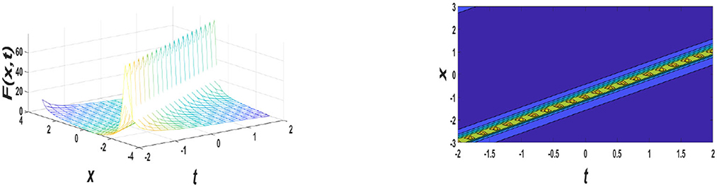
Figure 1. Graphs for μ = 0, σρ>0, σ = 0.2, ρ = 0.5, V = 1, A₁ = 0.1, A₂ = 0.2, −4 ≤ x ≤ 4, and −2 ≤ t ≤ 2 values of the Equation (33).

FIGURE 2

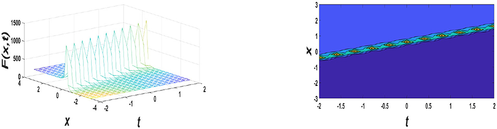
Figure 2. Graphs for μ = 0, σρ < 0, σ = 0.2, ρ = −0.3, V = 2, A₁ = 0.02, A₂ = 0.03, −4 ≤ x ≤ 4, and −2 ≤ t ≤ 2 values of the Equation (34).

FIGURE 3

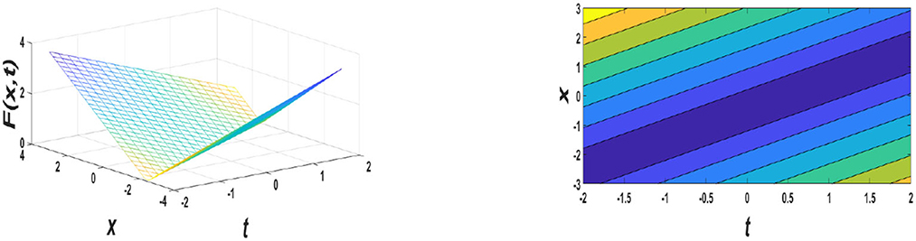
Figure 3. Graphs for A₁ = 0.02, ρ = 0.5, A₂ = 0.03, v = 1, −4 ≤ x ≤ 4, and −2 ≤ t ≤ 2 values of the Equation (35).

FIGURE 4

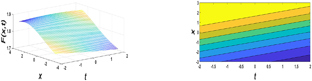
Figure 4. Graphs for μ = −0.3i, ρ = 0.15, σ = −0.2, V = 2, A₁ = 0.5, A₂ = 0.4, −4 ≤ x ≤ 4, and −2 ≤ t ≤ 2 values of the Equation (36).

FIGURE 5

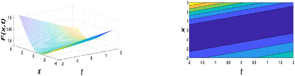
Figure 5. Graphs for μ ≠ 0, μ = 2, ρ = 1, σ = 2, V = 1, A₁ = 0.2, A₂ = 0.3, −4 ≤ x ≤ 4, and −2 ≤ t ≤ 2 values of the Equation (37).

7. Conclusion

Soliton solutions of nonlinear perturbed Schrödinger equation, that is, Equation (14) have been obtained from the estimated values of the GVD coefficient, and Kerr nonlinearly coefficient and their graphical simulations are presented. As shown in Figure 1, the amplitude of the soliton-like profile can be varied by altering the coefficients σ, μ, ρ, A₁, and A₂. As shown in Figure 2, considering the values of B, D, and A by altering the coefficients γ₁, γ₂, γ₃, σ, μ, ρ, A₁, and A₂, a bright profile can be realized. Moreover, soliton profiles can be realized by estimated values of A₁, A₂, γ₁, γ₂, γ₃, and ρ, which is shown in Figure 3. As shown in Figure 4, the kink-like profile can be realized for the estimated values of △₂, A₁, A₂, γ₁, γ₂, and γ₃. In Figure 5, the amplitude and spread of the dark soliton profile can be varied by altering the coefficients △₁, A₁, and A₂. These figures demonstrate the variation in amplitudes of fast compressive solitons reduces sharply in the small lower zone, and subsequently decreases slowly in the higher regime. However, the widths of the opposite trend are seen in the right moving solitons as Figures 1, 3. To the best of our knowledge concern from the literature, some of the results are new and have not been reported previously, and some are converging such as the wave profile of the left side of Figure 2 is having similar nature to Figure 2 of Yanjie et al. [34]. We do believe that our results may be helpful for the additional investigation of the propagation of the wave in optical MMs. In optical communication technology, solitons play an important role, significantly low bit error rate (BER) along with its strongly anti-interference ability is the reason why optical solitons are being used as a carrier wave of ultra-high-speed signals with no distortion.

Data availability statement

The raw data supporting the conclusions of this article will be made available by the authors, without undue reservation.

Author contributions

The author confirms being the sole contributor of this work and has approved it for publication.

Conflict of interest

The author declares that the research was conducted in the absence of any commercial or financial relationships that could be construed as a potential conflict of interest.

Publisher's note

All claims expressed in this article are solely those of the authors and do not necessarily represent those of their affiliated organizations, or those of the publisher, the editors and the reviewers. Any product that may be evaluated in this article, or claim that may be made by its manufacturer, is not guaranteed or endorsed by the publisher.

References

1. Yan C. A simple transformation for nonlinear waves. Phys Lett A. (1996) 224:77–84. doi: 10.1016/S0375-9601(96)00770-0

CrossRef Full Text | Google Scholar

2. Belgacem FBM, Bulut H, Baskonus HM, Akturk T. Mathematical analysis of the generalized Benjamin and Burger-KdV equations via the extended trial equation method. J Assoc Arab Univ Basic Appl. (2014) 16:91–100. doi: 10.1016/j.jaubas.2013.07.005

CrossRef Full Text | Google Scholar

3. Yan Z, Zhang H. New explicit and exact travelling wave solutions for a system of variant Boussinesq equations in mathematical physics. Phys Lett A. (1999) 252:291–6. doi: 10.1016/S0375-9601(98)00956-6

CrossRef Full Text | Google Scholar

4. Jafari H, Sooraki A, Khalique C. Dark solitons of the Biswas-Milovic equation by the first integral method. Optik. (2013) 124:3929–32. doi: 10.1016/j.ijleo.2012.11.039

CrossRef Full Text | Google Scholar

5. Biswas A. 1-Soliton solution of the K(m, n) equation with generalized evolution. Phys Lett A. (2008) 372:4601–2. doi: 10.1016/j.physleta.2008.05.002

CrossRef Full Text | Google Scholar

6. Ma WX. Travelling wave solutions to a seventh order generalized KdV equation. Phys Lett A. (1993) 180:221–4. doi: 10.1016/0375-9601(93)90699-Z

CrossRef Full Text | Google Scholar

7. Malfliet W. Solitary wave solutions of nonlinear wave equations. Am J Phys. (1992) 60:650–4. doi: 10.1119/1.17120

PubMed Abstract | CrossRef Full Text | Google Scholar

8. Ahmad H, Seadawy AR, Khan TA. Numerical solution of Korteweg-de vries-burgers equation by the modified variational iteration Algorithm-II arising in shallow water waves. Phys Scripta. (2020) 95:045210. doi: 10.1088/1402-4896/ab6070

CrossRef Full Text | Google Scholar

9. Wang X, Li J. The $\frac{G}{G^{\prime }}$-expansion method and travelling wave solutions of nonlinear evolution equations in mathematical physics. Phys Lett A. (2008) 372:417–23. doi: 10.1016/j.physleta.2007.07.051

CrossRef Full Text | Google Scholar

10. Qawasmeh A, Alquran M. Soliton and periodic solutions for (2+1)-dimensional dispersive long water-wave system. Appl Math Sci. (2014) 8:2455–63. doi: 10.12988/ams.2014.43170

CrossRef Full Text | Google Scholar

11. Alquran M, Qawasmeh A. Soliton solutions of shallow water wave equations by means of $(\frac{G^{\prime }}{G})$-expansion method. J Appl Anal Comput. (2014) 4:221–9. doi: 10.11948/2014010

CrossRef Full Text | Google Scholar

12. Li LX, Li EQ, Wang ML. The $(\frac{G^{\prime }}{G},\frac{1}{G})$-expansion method and its application to travelling wave solutions of the Zakharov equations. Appl Math J Chin Univ. (2010) 25:454–62. doi: 10.1007/s11766-010-2128-x

CrossRef Full Text | Google Scholar

13. Feng ZS. The first integral method to study the BurgersKdV equation. J Phys A Math Gen. (2002) 35:343–9. doi: 10.1088/0305-4470/35/2/312

CrossRef Full Text | Google Scholar

14. Kudryashov NA. Simplest equation method to look for exact solutions of nonlinear differential equations. Chaos Solitons Fract. (2005) 24:1217–31. doi: 10.1016/j.chaos.2004.09.109

CrossRef Full Text | Google Scholar

15. Antonova AO, Kudryashov NA. Generalization of the simplest equation method for nonlinear non-autonomous differential equations. Commun Nonlinear Sci Numer Simulat. (2014) 19:4037–41. doi: 10.1016/j.cnsns.2014.03.035

CrossRef Full Text | Google Scholar

16. Kudryashov NA. On nonlinear differential equation with exact solutions having various pole orders. Chaos Solitons Fract. (2015) 75:173–7. doi: 10.1016/j.chaos.2015.02.016

CrossRef Full Text | Google Scholar

17. Kudryashov NA. Painlevé analysis and exact solutions of the Korteweg-de Vries equation with a source. Appl Math Lett. (2015) 41:41–5. doi: 10.1016/j.aml.2014.10.015

CrossRef Full Text | Google Scholar

18. Jawad AJM, Petkovic MD, Biswas A. Modified simple equation method for nonlinear evolution equations. Appl Math. Comput. (2010) 217:869–77. doi: 10.1016/j.amc.2010.06.030

PubMed Abstract | CrossRef Full Text | Google Scholar

19. Cinar M, Onder I, Secer A, Yusuf A, Sulaiman TA, Bayram M, et al. The analytical solutions of Zoomeron equation via extended rational sin-cos and sinh-cosh methods. Phys Scripta. (2021) 96:094002. doi: 10.1088/1402-4896/ac0374

CrossRef Full Text | Google Scholar

20. Aljahdaly NH. Some applications of the modified $(\frac{G^{\prime }}{G^2})$ -expansion method in mathematical physics. Results Phys. (2019) 13:102272. doi: 10.1016/j.rinp.2019.102272

CrossRef Full Text | Google Scholar

21. Behera S, Aljahdaly NH, Virdi JPS. On the modified $(\frac{G^{\prime }}{G^2})$-expansion method for finding some analytical solutions of the traveling waves. J Ocean Eng Sci. (2022) 7:313–20. doi: 10.1016/j.joes.2021.08.013

CrossRef Full Text | Google Scholar

22. Yao SW, Behera S, Inc M, Rezazadeh H, Virdi JPS, Mahmoud W, et al. Analytical solutions of conformable Drienfeld-Sokolova-Wilson equation via sine-cosine method. Results Phys. (2022) 42:105990. doi: 10.1016/j.rinp.2022.105990

CrossRef Full Text

23. Wen AL, Hao C, Guo CZ. The $\frac{w}{g}$-expansion method and its application to vakhnenko equation. Chin Phys B. (2009) 18:400. doi: 10.1088/1674-1056/18/2/004

CrossRef Full Text | Google Scholar

24. Arshed S, Sadia M. $(\frac{G^{\prime }}{G^2})$-expansion method: new traveling wave solutions for some nonlinear fractional partial differential equations. Opt Quant Electron. (2017) 50:123. doi: 10.1007/s11082-018-1391-6

CrossRef Full Text

25. Zhang Z. New exact solutions to be generalized nonlinear Schrödinger equation. Phys Rev E. (2008) 17:125–34.

Google Scholar

26. Shehata R. The traveling wave solutions of the perturbed nonlinear Schrödinger equation and the cubic-quintic Ginzburg Landau equation using the modified $(\frac{G}{G^{\prime }})$-expansion method. Appl Math Comp. (2010) 217:1–10. doi: 10.1016/j.amc.2010.03.047

CrossRef Full Text | Google Scholar

27. Chen X. On the rigorous derivation of the 3D cubic nonlinear Schrödinger r equation with a quadratic trap. Arch Ration Mech Anal. (2013) 210:365–40. doi: 10.1007/s00205-013-0645-5

CrossRef Full Text | Google Scholar

28. Biswas A, Konar S. Introduction to Non-Kerr Low Optical Solitons. Boca Raton, FL: CRC Press (2007).

Google Scholar

29. Shabat A, Zakharov V. Exact theory of two-dimensional self-focusing and one-dimensional self-modulation of waves in nonlinear media. Sov. Phys. JETP, (1972) 34:62.

Google Scholar

30. Ablowitz MJ, David JK, Alan CN. Coherent pulse propagation, a dispersive, irreversible phenomenon. J Math Phys. (1974) 15:1852–8.

Google Scholar

31. Yu W, Ekici M, Mirzazadeh M, Zhou Q, Liu W. Periodic oscillations of dark solitons in nonlinear optics. Optik. (2018) 165:341. doi: 10.1016/j.ijleo.2018.03.137

PubMed Abstract | CrossRef Full Text | Google Scholar

32. Christiansen PL, Sϕrensen MP, Scott AC. Nonlinear Science at the Dawn of the 21st Century. Springer (2000).

Google Scholar

33. Liu Z, Li Q, Lin Q. New bounded traveling waves of Camassa-Holm equation. Int J Bifurcat Chaos. (2004) 14:3541–56. doi: 10.1142/S0218127404011521

CrossRef Full Text | Google Scholar

34. Wen Y, Xie Y. Exact solution of perturbed nonlinear Schrödinger equation using $(\frac{G^{\prime }}{G},\frac{1}{G})$-expansion method. Pramana J Phys. (2020) 94:18. doi: 10.1007/s12043-019-1875-3

CrossRef Full Text | Google Scholar

35. Abdelwahed HG, El-Shewy EK, Alghanim S, Abdelrahman MAE. Modulations of some physical parameters in a nonlinear Schrödinger type equation in fiber communications. Results Phys. (2022) 38:105548. doi: 10.1016/j.rinp.2022.105548

CrossRef Full Text | Google Scholar

36. Abdelrahman MAE, Hassan SZ, Alsaleh DM, Alomair RA. The new structures of stochastic solutions for the nonlinear Schrödinger's equations. J Low Frequency Noise Vibrat Active Control. (2022) 2022:14613484221095280. doi: 10.1177/14613484221095280

CrossRef Full Text | Google Scholar

37. Hosseini K, Ansari R, Samadani F, Zabihi A, Shafaroody A, Mirzazadeh M. High-order dispersive cubic-quintic Schrödinger equation and its exact solutions. Acta Physica Polonica A. (2019) 136:1. doi: 10.12693/APhysPolA.136.203

CrossRef Full Text | Google Scholar